The Jacobs Robotics Approach to Object Recognition and Localization
in the Context of the ICRA’11 Solutions in Perception Challenge
Narunas Vaskevicius Kaustubh Pathak Alexandru Ichim Andreas Birk
Abstract— In this paper, we give an overview of the Jacobs Robotics entry to the ICRA’11 Solutions in Perception Challenge. We present our multi-pronged strategy for object recognition and localization based on the integrated geometric and visual information available from the Kinect sensor. Firstly, the range image is over-segmented using an edge-detection algorithm and regions of interest are extracted based on a simple shape-analysis per segment. Then, these selected regions of the scene are matched with known objects using visual features and their distribution in 3D space. Finally, generated hypotheses about the positions of the objects are tested by back-projecting learned 3D models to the scene using estimated transformations and sensor model. Our method won the second place among eight competing algorithms, only marginally losing to the winner.
I. Introduction
This paper gives an overview of the approach used by the Jacobs Robotics team in the ICRA 2011 Solutions in Perception Challenge. Object recognition has been long studied in general and it recently found quite some attention with respect to the use of combined RGB and depth information - especially in form of Kinect data [1], [2], [3], [4], [5]. Due to space limitations, we focus in this paper on the technical description of our methods and an in-depth discussion of the general state of the art is omitted; the literature references are hence limited to a minimum to point to the work on which we build upon and to indicate where we extend it.
The paper is organized in the following way. Firstly, we introduce
our notation, used throughout the paper, in Sec. I-A. Then an
overview of the object recognition system is given in Sec. II.
The subsequent sections have detailed description of each of the introduced components and the underlying algorithms. The exper-imental setup and comprehensive benchmarking on two data-sets from ICRA 2011 Solutions in Perception Challenge is provided in
Sec.VII. Finally, concluding remarks are presented in section Sec.
VIII.
A. Notation
The notation used in this paper is summarized in Table I. In
general, scalars are in normal lowercase letters, vectors in bold small letters, and matrices in bold capitals. For quantities resolved in di↵erent frames, we use the left superscript/subscript notation of
[6]. Right subscripts are used for indexing or for denoting vector components.
Using this notation, the position vectors of the same physical
point observed from two di↵erent frames Fi and Fj with their
The authors are with the Dept. of EECS, Jacobs University
Bre-men, 28751 BreBre-men, Germany.{n.vaskevicius, k.pathak, a.birk}
@jacobs-university.de
The research leading to the results presented here has received funding from the European Community’s Seventh Framework Programme (EU FP7 ICT-2) within the project “Cognitive Robot for Automation Logistics Processes (RobLog)”.
TABLE I Notation p
i 2R3 Position vector of a spatial point resolved in the reference
frameFi.
p
i 2R4 The homogeneous coordinates for ip.
M
i Original image taken from camera-frameF
i.
m
i 2R2 Image pixel coordinates of a point in an image taken from
the camera-frameFi.
m
i 2R3 The homogeneous coordinates for im.
c
i 2R2 Normalized camera coordinates of a point in an image
taken from camera-frameFi.
c
i 2R3 The homogeneous coordinates for ic.
origins atOi andOjrespectively, are related by
p i = ijTjp, where, (1a) T i j , "iR j ijt 0T 3 1 # , it j ,OiO!j resolved inFi. (1b)
Using' to show equality up to a positive scale-factor and the
camera intrinsic parameter [7] matrixC, the camera model is given
by c i ,C 1im, ic' ip, (2a) m i ('1)ChiR j ijt i p j , ic' iR j jp+ ijt, (2b)
II. Design of theRecognitionSystem
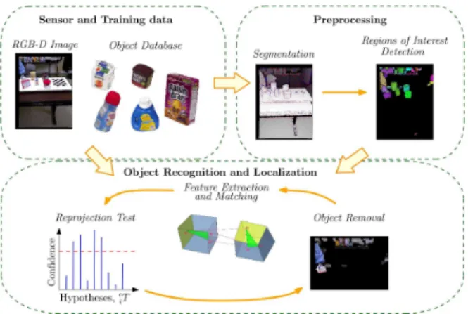
The workflow of the recognition system for detecting and
local-izing objects from a single view-point is depicted in Fig.1. The
recognition is done by combining texture information obtained from a color-image with geometric properties of the scene observed in a depth-image. For that, object database of point-cloud based 3D models with visual and shape cues is created during the training
phase (Sec.III). These models are then used to generate hypotheses
about the objects in the observed environment. This is done in the following way.
Segmentation.Firstly, the geometric properties of sensor data are examined by dividing range-image into regions of smooth surface
patches. This is achieved by the algorithm described in Sec.IV. A
very important aspect of our approach is the over-segmentation of the scene. In other words, there is no commonly used assumption that a segment must represent the whole object, which usually limits recognition to environments with well-separated objects on an easily detectable support surface, such as a table-top. On the contrary, finding smooth sub-segments of the objects is a plausible task even in cluttered scenes.
Regions of Interest.As described in Sec.IV-Athe segmentation result can be used to filter out large parts of the sensor data. Shape properties of a patch can be compared against those of the learned models to check if the segment could possibly be a part of any
ob-ject from the database. E↵ectively, large planar surfaces (e.g. walls,
floor, table-tops etc.) or other geometrically inconsistent segments 2012 IEEE International Conference on Robotics and Automation
RiverCentre, Saint Paul, Minnesota, USA May 14-18, 2012
Fig. 1. Object recognition and localization in a single RGB-D frame
are removed and not considered in the recognition process. The detection of regions of interest significantly reduces search space for recognition and localization algorithm, but is completely optional.
Feature Extraction and Matching.After the preprocessing step, we combine the regions of interest into a global mask and use it for extraction of texture features (e.g. Speeded Up Robust Features (SURF) [8], [9], the Scale Invariant Feature Transform (SIFT) [10],
etc.). As explained in Sec. V each feature descriptor vector is
associated with a 3D pose with respect to the range sensor. Then, the hypothesis about the best position in the scene is generated for each object using random sample consensus (RANSAC) [11] based
feature-matching with 3D geometric constraints (Algorithm2).
Testing Hypotheses.The transforms computed by the matching algorithm are used to re-project the models of the objects. Color and
range consistency tests (Sec.VI) are then used to filter out
false-positives. Objects with high consistency scores are considered to be recognized and their corresponding regions of interest are removed from the scene. Detection is then re-iterated on the remaining segments to handle multiple instances of the same object.
III. 3D Models ofReal-WorldObjects
This section describes the model used by the recognition system to represent real-world ojects.
We use a set of 3D points sampled from the object’s surface paired with the colors at their locations to model the shape and appearance of the real-world instance:
P,P⇥C=nhp,ci| p2P,R3,c2Co. (3)
HereCdenotes a color space e.g.RGB,CIE L*A*B*, etc.
The following quantities are calculated using Principal
Com-ponent Analysis (PCA) on the point-cloud P to describe the
dimensions of the object:
min,2·3p min, max,2·3p max, (4a) d,1
2·6
p
med+ min, (4b)
where, max, med, min are sorted eigenvalues of the covariance
matrix calculated during PCA. min and max are respectively the
minimum and maximum extent of the object. The PCA on the set
P can be viewed as an ellipsoidal approximation of the object’s
shape. Thus, the diameter d of gyration of the ellipsoid about
the principle PCA axis can be interpreted as the approximate
diameter of the object. As described in Sec.IV-A, these three values
Fig. 2. A model of the Silk Original soy milk carton on the left and the corresponding SURF feature locations on the right.
⌃,{ min, max, d}are used to find regions of interest during the
recognition phase.
In addition to the geometric properties, the model also contains a set of local invariant texture features [12].
D,D⇥P=nhd(n),pi |d(n)2Rn,p2Po (5)
The n-dimensional feature descriptor vectorsd(n)are coupled with
their locations on the object to aid feature matching and localization steps (Sec.V).
Thus, the object model is defined by the 3-tuplehP,D,⌃i. The
example of a model for one of the objects from Solutions in
Perception Challenge data-set is illustrated in Fig.2. The transparent
ellipsoid represents the three-sigma PCA approximation of the object’s shape. Its minor, medial and major axes are demonstrated respectively by red, green and blue arrows. The purple circle
surrounding the object has the radius of d.
IV. Segmentation
Segmentation is the process of dividing a range-image into connected components or segments, each of which is a smooth surface patch which is separated from its neighbors by jump or crease edges. A jump edge is formed when two neighboring
segments have a physical separation causing aC0discontinuity in
the range values. A crease edge, on the other hand, is aC1
range-discontinuity between segments which physically touch along the edge. Each segment represents a facet – not necessarily planar – of an object in the scene.
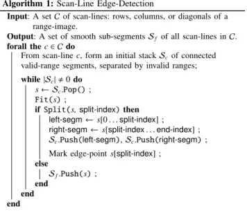
The segmentation algorithm devised by us is an extension of
that presented in [13] and is summarized in Algorithm1. A
scan-line in a range-image is defined as either a row, a column, or a diagonal (ascending or descending) of the range-image. Each scan-line is processed separately, and is split into curve-segments using the method of [14], also known as the Ramer-Douglas-Peucker
algorithm. Essentially, a scan-line can be considered as apiece-wise
smooth mapping from the scan-line pixel-indexx2Zto the range
or depth valuez2R. Algorithm1is used to find this mapping: in
other words, it finds the edge-points which separate the scan-line
into sub-segments, each of which is a smooth functionz= fi(x).
Two main functions of the Algorithm1areFitandSplit.
In theFitfunction, a polynomial is fitted to a given sub-segment
of a scan-line. This can be done in several ways.
• Simple linear (SL) or quadratic (SQ):For the linear version, the first and last points of the sub-segment are used to fit a
Algorithm 1:Scan-Line Edge-Detection
Input: A setCof scan-lines: rows, columns, or diagonals of a
range-image.
Output: A set of smooth sub-segmentsSf of all scan-lines inC.
forall thec2Cdo
From scan-linec, form an initial stackScof connected
valid-range segments, separated by invalid ranges; while|Sc|,0do
s Sc.Pop();
Fit(s);
ifSplit(s,split-index)then
left-segm s[0. . .split-index] ;
right-segm s[split-index. . .end-index] ;
Sc.Push(left-segm),Sc.Push(right-segm);
Mark edge-points[split-index] ; else
Sf.Push(s);
end end end
unique line; for the quadratic version, the mid-point is also added to fit a unique quadratic polynomial.
• Least-squares linear (LSL) or quadratic (LSQ):All points in the sub-segment are considered, and a linear or a quadratic polynomial is fitted using a standard least-squares method, minimizing the sum of algebraic residuals.
• Adaptive (AD):This is our extension of the algorithm. Recall that for a least-squares model-fitting – assuming a constant
known Gaussian noise with variance 2 in all samples – the
Akaike Information Criterion (AIC), and its corrected version for small sample-size (AICc) [15], for the model-fit may be defined as AIC{ri},K,N =2K+ 12 N X i=1 r2 i 2C, (6) AICc=AIC+ 2K(K+1) (N K 1), (7)
where, K is the number of parameters in the model, C is a
constant, depending only on the known parameter 2,Nis the
number of samples, andri is the least-squares fitting residual
for the samplei.
The adaptive strategy consists of fitting a least-squares linear
polynomial (K=2) on the sub-segment, followed by fitting a
least-squares quadratic polynomial (K=3), and selecting the
one with the lower value of AICc.
The functionSplitconsists of checking if a sub-segment sof
a scan-line c can be spit further into subsegments, and if so, at
which x. This xvalue is denoted bysplit-index. The function
returns true, if the splitting is to take place. For a sub-segment
to be considered for further splitting, it should have at least min
points. There are two main splitting strategies.
• Maximum residual (MR):The candidate splitting point in the
sub-segment is the one with the maximum residual rm from
the fitted polynomial. The splitting is done ifrm>✏, where✏
depends on the noise level of the data. This strategy has been followed in [13]. Although in [13] both SQ and LSQ were used for fitting, they did not discuss an important problem which often arises when using LSQ with MR, namely, that many times the candidate split-point turns out to be the very
TABLE II MainEdge-DetectionModes.
Mode Fitting Splitting Time (s)
Simple-Linear SL MR 2.3 Simple-Quadratic SQ MR 2.3 LS-AICC AD MAIC 13.1 LS-Mixed SQ+AD MR+MAIC 3.5
first point of the sub-segment. This does not occur when using SQ with MR as the residual at the end-points is explicitly
zero. We have hence concluded that LSQ+MR is not a good
combination.
• Minimum AICc (MAIC): This is our extension of the
algo-rithm. For a sub-segment s, after doing an adaptive fitting,
all points where the residual achieves a local maximum are considered potential splitting points. We consider all of these potential points in turn, and compute the decrease in AICc on hypothetically splitting the segment at that point. If none of the candidates lead to a decrease in AICc as compared to the un-split segment, no splitting is performed; else, the candidate which leads to the most decrease is selected as the splitting point. Note that fitting for all subsegments is done adaptively, i.e. their number of parameters is adaptively selected. Based on the above description, and after doing some experimen-tation, we came up with four combined strategies for comparison,
as listed in TableII. The runtime listed is for the processing of the
whole image, i.e. for all rows, columns, and diagonals. In mode
LS-Mixed, fitting and splitting strategies are based on those of Simple-Quadraticinitially; after the segment size reduces below minfmixed,
the strategy switches to that ofLS-AICC. This strategy is thus a
compromise in the trade-o↵between quality and computation time,
and hence is our default strategy due to its good results. Please
refer to Fig.3(b)for the quality of edge-detection on range images
collected using the Kinect sensor with the parameters✏= =0.015
m, min=4 and fmixed=12. The switching of strategies was done
when a sub-segment size had reduced to 48 pixels.
A. Filtering-out and Smoothing Objects of Interest
The edge-points in the left sub-figures of Fig.3do not yet form
closed boundaries of the object surface patches they demarcate. To achieve this, certain morphological transforms, as implemented in OpenCV [16], are applied, which is also done in [13]. In particular, an erosion with a kernel size of 5 followed by a dilation with a kernel size of 3 gave satisfatory separation of connected components for the 3D sensor employed.
From the training phase, the algorithm has good estimates of the dimensions of the objects it is looking for. The sizes of all trained objects are used to come up with minimum and maximum thresholds, which can be used to filter out extraneous objects and the background. Any predominantly planar objects which are significantly bigger than the thresholds are filtered out first. This is accomplished by first applying a distance-transform (DST implementation in OpenCV) on the edge-points image: the peaks of the resulting image give points which are far away from the edges and hence are good seeds to grow planar patches from. A region-growing algorithm [17] was used to grow planar patches. All dominant planar patches, which cannot possibly be part of an object of interest due to their size, are filtered out irrespective of their orientation. This typically removes walls, table-tops, etc. and makes subsequent processing much simpler.
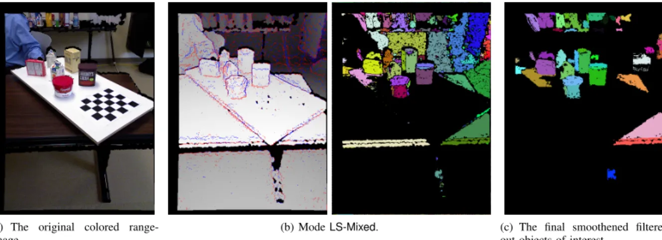
(a) The original colored
range-image. (b) ModeLS-Mixed. (c) The final smoothened filteredout objects of interest.
Fig. 3. Results of segmentation for one of the example test scenes. The left image in Fig.3(b)shows the found edge-points usingLS-Mixedmode.
The point-color denotes the convex/concave categorization of the edge w.r.t the view point. The images on the right show the color connected-components
representing object patches. Before running the connected-components algorithm a morphological transform was applied to clearly separate the components.
[18] is run to find potential object components as shown in the
right side sub-figure of Fig.3(b), where each component is given a
unique color. To these remaining connected components, Principal Component Analysis (PCA) is performed and components with dimensions not falling within the limits determined during the training phase are removed. Finally, we expand and smoothen the remaining components. This is done by fitting a 3D quadric surface [19] on a found component and testing its neighboring points to see if they satisfy the quadric equation within some bounds: if they do, they are made part of the component. This results in filling-in of holes and smoothing of the components which now represent object surface patches— these are shown in
Fig.3(c). Interestingly, the time taken for removing large planes,
finding connected-components, and filtering-out objects of interest,
followed by smoothing them, was 0.13 sec., which is a fraction
of the time required for scan-line edge-detection (TableII, mode
LS-Mixed).
V. FeatureExtraction andMatching
After the segmentation step the regions of interest are combined into a global mask. Then a standard feature extraction pipeline is applied on this image mask. Firstly, a set of distinctive keypoints is detected and then the region content around each of the keypoints is summarized in feature descriptor vectors. Instead of keeping keypoints defined in image coordinates, the corresponding 3D positions resolved in the object frame are calculated using relations
in equation (2b). The 3D keypoint-descriptor pairs define the set
Ds. Then for all objectsoiin model data-base, their feature-setDi
is matched against feature-set in the scene using Algorithm2.
The matching algorithm starts by finding a set of feature correspondence pairs between the object and the scene
-FindFeatureCorrespondences. For each feature vector ⌧j.d(n),
⌧j 2 Di the nearest neighbor ⌧?.d(n), ⌧? 2 Ds is found using
Euclidean distance in the feature space. If distance between features is small enough i.e.k⌧j.d(n) ⌧?.d(n)k< f, then the pairh⌧j,⌧?iis
added to the list of potential correspondences -Tf. Note that the
uniqueness of the closest feature is not tested. This is usually done using the ratio between the distances to the two closest features.
We have tried di↵erent strategies and the results were better when
the additional filtering by the ratio was not applied. Using only the nearest features increases both the number of correct and
Algorithm 2:RANSAC Based Feature Matching Input:Ds,Di
Output: sT
i andcmax- size of the maximum consensus set.
Tf FindFeatureCorrespondences(Ds,Di); Tf Sort(Tf); T↵ Filter(Tf,↵); forall thehs⌧1,o⌧1i 2T↵do T2 FindConsistent(hs⌧1,o⌧1i,Tf); T Filter(T2, ); forall thehs⌧2,o⌧2i 2T do T3 FindConsistent(hs⌧2,o⌧2i,T); hsT i j,cji RANSAC(T3, nr); ifcj>cnthen cn cj; T s i si jT; end end end
false correspondences. The higher rate of the false correspondence
pairs is acceptable since they are e↵ectively eliminated by the 3D
geometric constraints during the matching algorithm. The full set of
correspondencesTf is then sorted by the correspondence distance
and only↵% with the smallest distances are kept for the outer loop.
For each element hs⌧
1,o⌧1i 2 T↵ a set of geometrically
consistent correspondences is constructed. Two feature pairs hs⌧
1,o⌧1i,hs⌧2,o⌧2i 2Ds⇥Do are geometrically consistent if the
following equation is satisfied
⌧
s
2.p s⌧1.p = o⌧2.p o⌧1.p . (8)
This first test is based on the observation that if the object in the scene and its model have the same scale then the layout of the features with respect to each other is preserved. Thus the distances
from all model featureso⌧
j to a fixed featureo⌧1 are the same as
the distances of their correct counterparts in the scenes⌧
j to the
corresponding fixed features⌧
1.
After keeping the best % correspondences from theT2set the
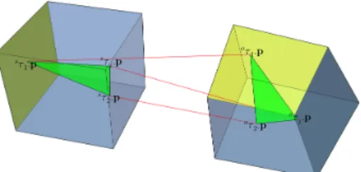
inner loop fixes the second correspondence pair -hs⌧2,o⌧2i 2T. The additional constraint introduced by the second pair allows us to further reduce the number of candidate correspondences. The
⌧ s 2.p ⌧ o 2.p ⌧ o 1.p ⌧ o j.p ⌧ s 1.p ⌧ s j.p
Fig. 4. If the objects in the scene and their models are of the same scale then the triangles formed by three correct correspondences are congruent
T3 is formed of the features geometrically consistent with the
fixed correspondences. The geometric constraints introduced by two
fixed correspondence pairs are illustrated in Fig.4. For any correct
correspondencehs⌧j,o⌧ji 2T the triangleshs⌧1.p,s⌧2.p,s⌧j.piand ho⌧
1.p,o⌧2.p,o⌧j.pihave to be congruent.
Though heavily pruned, the set T3 ⇢ Tf still might have
outliers due to the sensor noise and approximation by the parameter
f. Also, since only two correspondences were fixed, there still
might be geometrically inconsistent correspondences. To address these problems a standard RANSAC algorithm [11] is applied on
the setT3. Three correspondences are randomly selected and the
transformation sT
o between the model and the scene is estimated
using [20]. Then the consesus set is created: a feature pair is considered consistent if
⌧
s
j.p osTo⌧j.p d. (9)
Afternr iterations all correspondences in the largest consensus set
are used to recalculate the final estimatesT
o . The rate of outliers in
the setT3is very low. In most of the cases the largest consensus set
is equal toT3, therefore only few iterations are needed. As specified
in TableIIIwe have usednr=100.
The final result of the Algorithm 2 is the transformation
cal-culated using the largest consensus set obtained by fixing di↵
er-ent correspondences in the loops. The worst case computational
complexity for the object with feature setD isO(|D|3). However,
in practice, due to geometric constraints and parameters↵, and
f, the matching can be used in real-time applications even with
feature-sets of size up to 105.
VI. ReprojectionTest
The matching algorithm described in the previous section is
applied to all the modelsoj,j= 1. . .nin the training database.
Thus for each object an estimate of its best location in the scene
T
s
j is determined based on the largest consensus set with sizecj. In
many cases, if the object is not in the scene, even the minimum consensus set (of size 3) is not constructed due to the small initial correspondence set and geometric constraints. However the local feature descriptors and their configuration in 3D space are not always enough to distinguish objects uniquely; therefore false positives have to be eliminated.
The size of the consensus set could already be used as the criteria for discarding objects not present in the scene, but for which the location estimate has been generated. Unfortunately, the variation in the number of features per model is quite large. Less textured objects would have always small consensus sets even though they are present in the scene, whereas highly textured objects would usually have a larger subset of features which would be consistent with some part of the scene. Therefore, more complicated tests are needed for checking the hypotheses. For this, we perform a simulation of data collection using a sensor model and the
hypotheses generated by Algorithm2. The consistency between the
simulated data and the real measurements is then checked for the identification of the correct hypotheses.
As described in Sec. III, the object model oj is defined by
the three-tuple hPj,Dj,⌃ji. The set of colored points Pj can be
transformed to the sensor frame using the hypothesis about its location -sT
j . Using the camera model Eq. (??), these points can
be projected onto the image plane. We have used depth-bu↵er for
projecting only those parts of the object which are visible from the
position of the sensor. Thus for each objectojin the data-base, an
RGB-D imagesM j is generated. M s j(sm)= argmin ⌧ s 2sP(sm)k ⌧ s .pk, (10) P s (sm),ns⌧, hsT j j⌧.p,j⌧.ci| sm'Cs⌧.p o (11) Let Mj , {sm|9j⌧ 2 jP : sm ' C Tsj j⌧.p} be a set of discrete
image coordinates obtained by projecting object modeloj. Also we
denoteS={S1,S2, . . .Sn}to be a set of regions of interests obtained
after the segmentation described in Sec.IV. Each of the regions is
defined by a set of image coordinates. Then the following quantities are used to determine consistency between real and modeled data.
sd, P m2Mj1d{m, M s j(m)} |Mj| (12) sc, P m2Mj1c{m, M s j(m)} |Mj| (13) f(S), X m2Mj\S 1d{m,sMj(m)}^1c{m,sMj(m)} so, f(S ?) |S?| , S ?,argmax S2S f( S) (14)
The quantities defined in equations (12) and (13) respectively are
distance and color consistency measures. For each pixelmin the
mask Mj of the projected model consistency is checked using
indicator functions 1d{·} and 1c{·}. The depth similarity at pixel
mis evaluated by comparing the range values at the same pixel in
the simulated and the real RGB-D images:
1d(m,⌧),
(
1, |ksM(m).pk k⌧.pk|<"
d
0, else. (15)
Color consistency is checked using a small window of size 2w+1
around pixelmin the real range image:
1c(m,⌧),
(
1, 9b2Bw(m):ksM(b).c ⌧.ckc<"c
0, else ,
Bw(m),{b| |mu bu|w^|mv bv|w}. (16)
Where, k ·kc is a color similarity metric. We have used CIE
L*A*B*space where the perceptual di↵erence between colors can be
approximated by the Euclidean distance between the color vectors.
As it has already been discussed segmentsS2Sare assumed to
be subsegments of the objects, i.e. we assume over-segmentation. If the hypothesis about the object’s location is correct then there
must exist a segment with high consistency S? in the overlap
between reprojected model and the segments in the real image{S2
S|M\S,;}. This requirement is expressed in equation (14), where
functionf(·) measures overlap consistency by comparing colors and
ranges between simulated and real data. Using this function we
can calculate the last quantitysoneeded for the consistency test. It
measures coverage rate of the segment with the highest consistent overlap.
Fig. 5. A snapshot of all 35 objects from Willow Garage data-set on the left and a textured manufacturing part from NIST collection on the right [21]
Based on definitions (12), (13) and (14) the final consistency test is done using the following inequality.
(4c·sc+(1 4c)·sd)·so ✓c, (17)
where scalar 0 4c 1 is the weight factor for the color
consistency measure and the threshold 0 ✓c 1 is the lowest
allowed total consistency for the hypothesis to be considered
correct. Thus, if the inequality (17) holds then the object oj is
considered to be in the scene at location sT
j . If there are at least two
objects satisfying inequality (17), but having the same segmentS?
as the best overlaping region then only the object with the highest total conistency is considered to be detected.
So far we have described how to detect single instance of an object, however there might be multiple occurences of the same object in the scene. For detecting other instances of the same object we first remove corresponding segments of the recognized objects and then repeat the matching and reprojection steps with the remaining segments and objects with the total consistency higher
than ✓c/2. These steps are re-iterated until no more objects are
detected.
VII. Experiments andBenchmarking
The approach described in the previous sections has been tested in a context of Solutions in Perception Challenge at International Conference on Robotics and Automation 2011 [21]. This was the first competition and it concentrated on the recognition and localization in 3D of textured objects at close range (approximately within 2 meters). The challenge made use of Kinect sensor which is able to produce RGB-D image at one mega-pixel resolution.
The data used for the challenge consisted of two data-sets totaling 50 objects. The first set, henceforth WG data-set, of 35 common
household objects Fig.5was provided by researchers from Willow
Garage before the competition. It contained extensive training sequences for each of the objects and example test scenarios with multiple objects per scene. The second data-set, henceforth NIST data-set, containing 15 objects was hidden from the participants to test robustness and generality of the developed algorithms. It com-prised of textured manufacturing parts. Only single representitive example was available to the contestants before the testing phase of the competition. A picture of a typical object from the NIST
data-set is shown in Fig.5on the right-hand side.
The recognition software developed by the participants had to be submitted to the competition committee. The algorithms were then trained and tested on their servers using before undisclosed data-sets containing one or more trained objects per frame. The test sequence with objects from WG data-set comprised of 176 frames with 434 recognizable objects in total. The NIST data-set had 831 object instances distributed over 399 frames. Full data was published after the challenge and is available online [21].
TABLE III
Values of the main algorithm parameters used for the competition
Parameters Description Values
f, d Feature and distance similarity thresholds 1.0, 15 mm
nr,↵ Feature matching parameters 100, 0.1
w,4c,✓c Reprojection parameters 4, 0.6, 0.4
The performance of the algorithms was evaluated at each frame using combinatorial scoring function based on the recognition rate and localization precision. The recognition score was dependant on the number of correct detections (true positives), incorrect detections (false positives) and undetected objects (false negatives), whereas localization score linearly decreased with increasing de-viation of the pose estimate from the ground-truth. The detailed definitions of the contributing terms can be found in [21]. The final score of a team was expressed as percentage of the maximum possible score over all frames.
There are several implementation details to be mentioned before
proceeding to the results. Firstly, object models Sec.IIIwere created
using the training data provided by the committee of the compe-tition. It was recorded using Kinect sensor and Robot Operating System (ROS) [22]. Each of the textured objects was scanned
from di↵erent view-points using rotating support and fiducial for
estimation of the object-camera relation. The raw data had to be further processed to create models required by our algorithm. This included object segmentation, extraction of local invariant features, registration and some post-processing tasks. As the type
of visual features we have chosen SURF with dimensionn=128.
We have used OpenCV implementation for detecting key-points and computing descriptor vectors. The algorithm was optimized to produce the best performance within allowed time limit - 15 s. per frame.
Using the parameters listed in TableIII the algorithm achieved
the best score among all participants - 82.2% (682.61/831) on
NIST data-set and the second result 50.6% (219.94/434) on Willow
Garage data-set. The final combined score 66.41% took the second
place behind the best score 68.78% achieved by the team from
UC Berkeley. The number of true positives, false negatives, false positives, and the accuracy of position estimates were respectively
750, 81, 2, 86% for NIST and 301, 133, 50, 75.4% for WG test
sets. Note that only true positives are included in the calculation of the localization accuracy. Further details on the competition results can be found in [21].
The final decision about the presence of an object instance in the
scene is done using the reprojection parameter✓c. Therefore more
detailed analysis of the algorithm’s sensitivity to the variations of
the decision threshold is depicted in Fig.6.
VIII. Conclusions
In this work we have presented an approach to object recognition and localization using visual and geometric cues available from RGB-D data. In addition to aiding the standard pipeline of visual object recogntion with depth information we have extended segmen-tation algorithm [13] to achieve better performance. As it already was emphasized the parameters of the edge-detection algorithm were set to achieve over-segmentation. Finding sub-segments of the objects does not require strong assumptions about the environment and as it was shown in this paper it can be applied in many stages of the object recognition process. One of them is reprojection test which was introduced by us to test the hypotheses about the objects present in the scene.
0.0 0.1 0.2 0.3 0.4 0.5 0.6 0.7 0.8 0.9 1.0 Reprojection Threshold 0.0 0.1 0.2 0.3 0.4 0.5 0.6 0.7 0.8 0.9 1.0 Rate
Performance Dependency on Reprojection Parameter (Willow Garage)
Score Recall Precision 0.0 0.1 0.2 0.3 0.4 0.5 0.6 0.7 0.8 0.9 1.0 Reprojection Threshold 0.0 0.1 0.2 0.3 0.4 0.5 0.6 0.7 0.8 0.9 1.0 Rate
Performance Dependency on Reprojection Parameter (NIST)
Score Recall Precision 0.0 0.1 0.2 0.3 0.4 0.5 0.6 0.7 0.8 0.9 1.0 Reprojection Threshold 0.0 0.1 0.2 0.3 0.4 0.5 0.6 0.7 0.8 0.9 1.0 Rate
Performance Dependency on Reprojection Parameter (Combined)
Score Recall Precision
j
(a) Precision, recall, and score dependency on✓crespectively for WG, NIST and combined data-sets
0.0 0.2 0.4 0.6 0.8 1.0 Precision 0.0 0.2 0.4 0.6 0.8 1.0 R eca ll
Recall Curve (Willow Garage)
0.0 0.2 0.4 0.6 0.8 1.0 Precision 0.0 0.2 0.4 0.6 0.8 1.0 R eca ll
Recall Curve (NIST)
0.0 0.2 0.4 0.6 0.8 1.0 Precision 0.0 0.2 0.4 0.6 0.8 1.0 R eca ll
Recall Curve (Combined)
(b) Precision-recall curves for WG, NIST and combined data-sets
Fig. 6. Score dependency on the reprojection parameter✓cand related precision-recall curves. The dashed vertical lines and the red circles indicate the
parameter value✓c=0.4 used for the competition.
The algorithm showed a good performance among eight entries to the Solutions In Perception Challenge by achieving the second best
result, 66.41% of the maximum score, with only 2.37% di↵erence
from the first place.
References
[1] K. Lai, L. Bo, X. Ren, and D. Fox, “Sparse distance learning for object
recognition combining rgb and depth information,” inRobotics and
Automation (ICRA), 2011 IEEE International Conference on, 2011,
pp. 4007–4013.
[2] L. Bo, K. Lai, X. Ren, and D. Fox, “Object recognition with
hierarchi-cal kernel descriptors,” inComputer Vision and Pattern Recognition
(CVPR), 2011 IEEE Conference on, 2011, pp. 1729–1736.
[3] K. Lai, L. Bo, X. Ren, and D. Fox, “A large-scale hierarchical
multi-view rgb-d object dataset,” inRobotics and Automation (ICRA), 2011
IEEE International Conference on, 2011, pp. 1817–1824.
[4] N. Silberman and R. Fergus, “Indoor scene segmentation using a structured light sensor,” 2011.
[5] J. Knopp, M. Prasad, and L. V. Gool, “Scene cut: Class-specific
object detection and segmentation in 3d scenes,” in 3D Imaging,
Modeling, Processing, Visualization and Transmission (3DIMPVT),
2011 International Conference on, 2011, pp. 180–187.
[6] J. J. Craig,Introduction to robotics – Mechanics and control. Prentice
Hall, 2005.
[7] R. Elias, “Projective geometry for three-dimensional computer vision,”
in Seventh World Multiconference on Systemics, Cybernetics and
Informatics, vol. v, Orlando, Florida, 2003, pp. 99–104.
[8] H. Bay, A. Ess, T. Tuytelaars, and L. Van Gool, “Speeded-up robust
features (surf),”Computer Vision and Image Understanding, vol. 110,
no. 3, pp. 346–359, 2008.
[9] H. Bay, T. Tuytelaars, and L. Van Gool,SURF: Speeded Up Robust
Features Computer Vision ECCV 2006, ser. Lecture Notes in
Com-puter Science. Springer Berlin /Heidelberg, 2006, vol. 3951, pp.
404–417.
[10] D. G. Lowe, “Distinctive image features from scale-invariant
key-points,”International Journal of Computer Vision, vol. 60, no. 2, pp.
91–110, 2004.
[11] M. A. Fischler and R. C. Bolles, “Random sample consensus: a paradigm for model fitting with applications to image analysis and
automated cartography,” Graphics and Image Processing, vol. 24,
no. 6, pp. 381–395, 1981.
[12] T. Tuytelaars and K. Mikolajczyk, “Local invariant feature detectors:
A survey,”Foundations and Trends in Computer Graphics and Vision,
vol. 3, no. 3, pp. 177–280, 2007.
[13] X. Jiang and H. Bunke, “Edge detection in range images based on
scan line approximation,”Computer Vision and Image Understanding,
vol. 73, no. 2, pp. 183–199, 1999.
[14] R. O. Duda and P. E. Hart,Pattern Classification and Scene Analysis.
New York: Wiley, 1972.
[15] K. P. Burnham and D. R. Anderson, Model Selection and
Multi-model Inference: A Practical Information-Theoretic Approach, 2nd ed. Springer Verlag, 2002, iSBN 0-387-95364-7.
[16] G. Bradski and V. Pisarevsky, “Intel’s computer vision library: ap-plications in calibration, stereo segmentation, tracking, gesture, face
and object recognition,” inComputer Vision and Pattern Recognition,
2000. Proceedings. IEEE Conference on, vol. 2, 2000, pp. 796 –797
vol.2.
[17] N. Vaskevicius, A. Birk, K. Pathak, and S. Schwertfeger, “Efficient
Representation in 3D Environment Modeling for Planetary Robotic
Exploration,”Advanced Robotics, vol. 24, no. 8-9, pp. 1169–1197,
2010.
[18] L. Di Stefano and A. Bulgarelli, “A simple and efficient connected
components labeling algorithm,” inImage Analysis and Processing,
1999. Proceedings. International Conference on, 1999, pp. 322–327.
[19] N. Vaskevicius, K. Pathak, R. Pascanu, and A. Birk, “Extraction of
quadrics from noisy point-clouds using a sensor noise model,” inIEEE
International Conference on Robotics and Automation (ICRA). IEEE
Press, 2010.
[20] B. K. P. Horn, “Closed-form solution of absolute orientation using unit
quaternions,”Journal of the Optical Society of America A, vol. 4, pp.
629–642, 1987.
[21] “Solutions In Perception Challenge ICRA’11.” [Online]. Available: http://opencv.willowgarage.com/wiki/SolutionsInPerceptionChallenge
![Fig. 5. A snapshot of all 35 objects from Willow Garage data-set on the left and a textured manufacturing part from NIST collection on the right [21]](https://thumb-us.123doks.com/thumbv2/123dok_us/703178.2587014/6.892.80.431.132.266/snapshot-objects-willow-garage-textured-manufacturing-nist-collection.webp)
