Modelling Network Traffic Via a Multifractal Wavelet Model. Christopher Peart

(1)

Modelling Network Traffic Via a Multifractal Wavelet

Model.

Christopher Peart

Dissertation submitted for a MSc in Networks, Non-linear dynamics and Data Analysis. Department of Mathematics

University of York August 2005

(2)

Introduction

Broadband band network traffic can not be modelled by the traditional pois-son approach. This is because network traffic exhibits long range dependence. Poisson models however, assume that the process is memoryless. This led to an influx of reseach into modelling long range dependence in network traffic.

Network traffic loads exhibit fractal properties such as long range dependence, self-similarity and burstiness. Therefore the challange in modelling network traffic is to develop a model which can capture these fractal properties.

Self-similar processes exhibit long range dependence and burstiness over dif-ferent time scales. Long range dependence is correlation in the data over a large time scale. However, in a long range dependent processes we have long term correlation but also can have some short term correlation which is different to the overall long term behaviour. Multifractal processes exhibit long range de-pendence and burstiness while showing varying scaling properties over differing time scales. For this reason a process can be multifractal but not self-similar. However, self-similar process are multifractal.

Fractal models have had large affect on network trafic modelling. In [9] it is shown the network traffic shows fratcal properties such as long range dependence, burstiness and self-similarity. It has been shown by [10] that the interarrival times of network traffic can modelled by multifractals. Multifractal models are suited to explain multiple scaling at different time scales and can also characterise burstiness in the traffic. Traditionally the analytic tractabiltiy of multifractal models is poor. However, our parametric wavelet model based on multifractal processes is analyticaly tractable and is used to model broadband traffic.

This model uses the Haar wavelet transform and a multiplicative structure for the wavelet and scaling coefficients to maintain a positive output. The model’s algorithm for synthesising data is rapid and is of O(N) to generate a N point data set. The model is an example of a binomial casscade. It effictively matches synthesised data to real time series.

In this dissertation we start by outlining the properties of self-similarity, long range dependence, heavy tailed distributions and general stochastic processes. We introduce the idea of multiplicative casscades and the multifracl spectrum. We go on to develop statistical techniques for analysing multifractal network traffic. We intruduce the multifractal wavelet model and apply it to the Bellcore data

(5)

set which we have shown is multifractal. Finally we consider a one dimensional map as a model for multifractal network traffic.

The matlab code to implement the multifractal model was taken from the website of R Riedi. The binomial cascade code adpated from [13]. The remaining code was written by myself.

(6)

CHAPTER 2

Preliminaries

The section on stochastic processes was based on [2], [6] and [1]. The section on long range dependence, self-similarity, fBm and heavy tailed processes were based on [1], [6] and [7].

In order to model network traffic we are concerned with the arrival times of packets of information. The length of time between arrivals of consecutive packets is called the interarrival time. The interarrival times of packets in network traffic is a stochastic process.

Definition _2.1. _{A sequence of random events variables}_{_X₍_t₎_{, t} _∈_T_} _where

the parametert is in the set T is a stochastic process.

The parameter t can be discrete or continuous which in turn causes the sto-castic process to be a discrete or continuous process.

Definition _2.2. Let X(t)be a stochastic process, X(t) is discrete valued if the set of all possible values of X(t) is countable. Otherwise we say that it is continuous.

Definition _2.3. _{The variance of a discrete or continuous random variable is}

defined as follows and is denotedσ2_,

σ2 =E[(X₋µ)2]. where µ=E(X) is the mean of X.

Definition _2.4. _{The autocovariance for a stochastic process} _X₍_t₎ _{is defined}

as,

γ(t, s) = E[X(t)X(s)] =E[(X(t)₋µ(t))(X(s)₋µ(s))] 1. Stationarity

Suppose we have a stochastic process where the pdf does not change with time then this implies that at any instant we observe the same random variable as at any other instant. This concept is known as stationarity.

Definition_2.5. LetX(t)be a stochastic process and denote its pdf byfX(t)(x). A stochastic process X(t) is stationary if and only if _∀ time instants t1, . . . , tk

and for anyk _∈N

fX(t1),...,X(tk)(x1, . . . , xk) =fX(t1+τ),...,X(tk+τ)(x1, . . . , xk) for anyτ >0.

(7)

This is sometimes called strict sense stationary. There is a theorem which is an immediate consequence of stationarity.

Definition _2.6. _Let _X₍_t₎ _{be a stationary stochastic process then:}

(1) E[X(t)] =µ is constant

(2) V ar[X(t)] is constant

(3) The covariance of any twoX(t1)and X(t2) depends only on t2 =t1+τ,

covariance depends only on τ.

The above conditions are necessary but not sufficient conditions for station-arity. They suggest possible ways in which we might determine the stationarity of a data set.

If a stochastic process fits the above conditions we say that it is wide sense stationary. This is a slightly weaker version of stationarity than given above. In practice, showing that a process is strict sense stationary is difficult.

2. Independent Increment Processes

In this dissertation we are trying to model interarrival times of packets in network traffic. The interarrival times in network traffic are examples of inde-pendent increments. Say thatX(t) is the random process of the interarrival times of network traffic. The increments of the process at time intervalst1, t2, . . . , tnare defined asX(t1)₋X(t0), X(t2)₋X(t1), . . . , X(tn)₋X(tn−1).The increments we

will be studying are those which are not affected by past and future increments, i.e. they are independent.

Definition _2.7. A stochastic process X(t) where 0 _≤ t0 ≤ t1 ≤ t2 ≤ · · · ≤

tn≤ ∞ is a independent increment process. If (1) X(0) = 0

(2) X(t2)₋X(t1), . . . , X(tn)₋X(tn−1) are independent.

For a stochastic process X(t) to have independent increments the process itself need not be independent.

For independant increment processes whose increments are stationary we have the following result.

Theorem₁. _{If a stocastic process}_X₍_t₎_{is a stationary independent increment}

process for 0_≤t _{≤ ∞} and we assume that the expectation of X(t) is zero then:

(1) E[(X(t)₋X(s))2_{] =}_σ2_|_t₋_s_| (2) E[X(t)X(s)] =σ2_min₍_{t, s}₎_.

(8)

2. INDEPENDENT INCREMENT PROCESSES 7

Proof. _{We first assume that} _X_{(0) = 0. Since the process has stationary}

increments this implies that:

E[X2(τ)] = E[(X(τ)₋X(0))2] = E[(X(τ +k)₋X(k))2].

Now we let τ and k equal the time steps t1 and t2 respectively we obtain

E[X2(t1)] = E[X2(t1+t2)] +E[X2(t2)]−2E[X(t1+t2)X(t2)].

The increments are non overlapping thereforeX(t2)₋X(t0) is not correlated to

X(t2+t1)−X(t2). We now look at the case when t0 = 0, hence X(t0) = 0 by our above assumption. This gives us that:

E[(X(t2−X(t0))(X(t2+t1)−X(t2))] = 0

E[(X(t2))(X(t2+t1)−X(t2))] = 0

E[X(t2)X(t1+t2)−X2(t2)] = 0

E[X(t2)X(t1+t2)] =E[X2(t2)]. Now substituting this into the earlier expression we have:

E[X2(t1] =E[X2(t1+t2)] +E[X2(t2)]−2E[X2(t2)] =E[X2(t1+t2)]−E[X2(t2)]

E[X2(t1+t2)] =E[X2(t1)] +E[X2(t2)].

Now let f(t) =E[X2₍_t_{)], then we can rewrite the above equation as follows:}

f(t1+t2) = f(t1) +f(t2). This relationship only possible iff(t) is linear

f(t) = E[X2₍_t_{)] =}_σ2_t.

Now letn < m, to calculateE[(X(m)₋X(n))2_{] we expand it using the rules of} expectation as follows.

E[(X(m)₋X(n))2] =E[X2(m)] +E[X2(n)]₋2E[X(m)X(n)] (2.1) =E[X2(m)] +E[X2(n)]₋2E[X2(n)] (2.2) =E[X2₍_m_)]₋_E_[_X2₍_n_)] _(2.3)

=σ2(m₋n) (2.4)

Form < n in a similar way we obtain the result

E[(X(m)₋X(n))2] =σ2(n₋m).

Now using both of these results we obtain the required result

E[(X(m)₋X(n))2] =σ2_|m₋n_|.

This proves the first part of the above result. For proof of the second part of the result we can use the early results obtained in the proof of part one. We

(9)

must obtain an expression for E[X(m)X(n)]. We first consider the case when

n < m, then

E[X(m)X(n)] =E[X2(n)] = σ2n

Since X(m)₋X(n) is independent of X(n). In the same way when m < n,

E[X(m)X(n)] =E[X2₍_m_{)] =}_σ2_m. Now putting both results together we have proved part two,

E[X(m)X(n)] = σ2min(m, n).

3. Self-Similar Process

A stochastic processX(t) with stationary increments is said to be self-similar if the following relation holds in distribution:

X(t+τ)₋X(t) =a−_H

[X(t+aτ)₋X(t)]

where the parameter H is known as the Hurst parameter. If we now impose the condition that t= 0 and use the fact that X(0) = 0, the self-similarity condition can be simplified to:

X(0 +τ)₋X(0) =a−_H

[X(0 +aτ)₋X(0)] (2.5)

X(τ) =da−_H

[X(aτ)] (2.6)

where again the relation holds in distribution.

A defining property of a fractal is that it exhibits self-similarity under differing scales. Therefore a self-similar process is known as a fractal process. The fractal dimension in this case is an indication of statistical nature of the data.

4. Variance Structure of a Self-similar Process

Let X(t) be a self-similar process with stationary increment, then we have the following result for X(t)

E[(X(t+τ)₋X(t))2] =Cτ2H

where C is a positive constant.

Proof. _{For a self-similar process} _X₍_t_{), using our definition of a self-similar}

process which is given above we have that:

E[(X(t+τ)₋X(t))2] =E[(a−_H

[X(t+aτ)₋X(t))2]].

If we now impose the initial conditionX(0) = 0, the above equation simplifies to

E[X2(τ)] =a−2H

E[X2(aτ)].

If we define a function to transform the above equation as follows,

f(τ) =a−_2H

(10)

6. LONG RANGE DEPENDENCE 9

Now let τ = 1 and substituting into (2.7) gives us:

f(1) =a−_2H

f(a) =_⇒ f(a) =a2Hf(1).

Now set f(t) =f(a) in the above equation gives,

f(t) =Ct2H; whereC =f(1). (2.8) Now we have that f(τ) = E[X2₍_τ_{)] =} _Cτ2H_{. Now using this and imposing the} intial comdition we have that:

E[(X(t+τ)₋X(t))2] =E[X2(τ)] imposing X(0) = 0 (2.9)

=f(τ) (2.10)

=Cτ2H. (2.11)

5. Covariance sturcture of a self-similar process

If X(t) is a self-similar process with stationary increments we can obtain the relation

E[(X(t)₋X(s))2] =E[X(t₋s)₋X(0))2] =σ2_|t₋s_|2H. (2.12) Now expanding both left and right hand sides of the above expressions gives,

E[((X(t)₋X(s))2] = E[X(t)2] +E[X(s)2]₋2E[X(t)X(s)] =σ2_|t₋s_|2H (2.13) Now using (2.8) we have thatf(t) =E[X2₍_t_{)] =} _σ2_t2H _{where we set} _C ₌_σ2_{, we} use this in (2.13) to get,

E[X(t)2] +E[X(s)2]₋2E[X(t)X(s)] =σ2t2H +σ2s2H ₋2γX(t, s). (2.14) Now using (2.12) and (2.14) we have that

σ2t2H +σ2s2H ₋2γX(t, s) = σ2|t−s|2H. (2.15) Now using (2.15) and making γX(t, s) the subject we can obtain the expression

γX(t, s) =

σ2 2 [t

2H

− |t₋s_|2H +s2H]. (2.16) 6. Long Range Dependence

Definition _2.8. The autocorrelation function or the ACF of a stationary increment processX(t) is defined as:

ρ(t, τ) =E[X(t)X(t+τ)].

Definition _2.9. The correlation coefficient of a stationary stochastic process X(t) is defined as,

ρ(k) = γX(X(0), X(k))

(11)

The property of long range dependence can be defined mathematically as follows.

Definition _2.10. Let X(t) be a stationary stochastic process then X(t) is said to be long range dependent if the absolute value of the autocorrelation, ρ(k), sum to infinity. Written mathematically as:

k=∞ X

k=−∞

ρ(k) =_∞ (2.17)

In order to define the long range dependence property we define a new sto-chastic process Y(t), as Y(t) = X(t)₋X(t₋1) this is a stationary increment process where t _∈ N_{. In order to define the long range dependence property} for this stationary increment process we examine the covariance of Y(t). The covariance of Y(t) is defined as:

E[Y(t+k)Y(t)] which we can rewrite in terms of X(t) as follows

E[Y(t+k)Y(t)] =E[(X(t+k)₋X(t+k₋1))(X(t)₋X(t₋1))].

Now using the rules of expectations we can bring the expectation inside the brackets to get that:

E[Y(t+k)Y(t)] = E[(X(t+k)₋X(t+k₋1))(X(t)₋X(t₋1))] =E[X(t+k)X(t)]₋E[X(t+k₋1)X(t)]₋

E[X(t+k)X(t₋1)] +E[X(t+k₋1)X(t₋1)].

Now we know that

γY(k) =E[Y(t+k)Y(t)]

is independent of t. Using the previous equation (2.16) we can rewrite our ex-pression for E[Y(t+k)Y(t)] as:

γY(k) =E[Y(t+k)Y(t)] =

σ2

2 [(k−1) 2H

−2k2H + (k+ 1)2H]. (2.18) Now in order to find the autocorrelation we use the defintion given above namely that:

ρ(k) = γY(k)

σ2 .

Now we can use equation (2.18) to obtain the following relation

ρ(k) = γY(k) σ2 = 1 2 (k₋1)2H ₋2k2H + (k+ 1)2H . (2.19) Now in order to examine the asymptotic behaviour of ρ(k), we can use the Taylor expansion. However, first we must modify equation (2.19) by taking a factor of k2H _{out of each term. This modification gives us:}

(12)

6. LONG RANGE DEPENDENCE 11 ρ(k) = k 2H 2 " 1 + 1 k 2H −2 + 1₋ 1 k 2H# (2.20) We now define a function which we can use for the Taylor expansion. Define

f(x) =

(1 +x)2H ₋2 + (1₋x)2H

.

Using this function we can rewrite our expression (2.20), for the autocorrelation, as, ρ(k) = k 2h 2 f(k −1 ). (2.21)

If we now recall the expression for the Taylor expandsion of a function f(x) around a point x0 as:

f(x₋x0) =f(x0) +xf 0 (x0) + x2 2 f 00 (x0) +. . . .

For us to be able to calculate the Taylor expansion of f(x) we must therefore calculate the derivatives:

f0 (x) = 2H (1 +x)2H−₁ −(1₋x)2H−₁ (2.22) f00 (x) = 2H(2H₋1) (1 +x)2H−₂ + (1₋x)2H−₂ . (2.23)

We will expand f(x) around the origin hence our expression for the Taylor series simplifies to: f(x) =f(0) +xf0 (0) + x 2 2 f 00 (0) +. . . .

We now substitute our expressions for the derivatives of f(x) and obtain:

f(x) = x 2

2 2H(2H−1) +O(x

3₎_. _(2.24)

Now combining (2.24) and (2.21) we can express ρ(k) as:

ρ(k) = k 2H 2 g(k −₁ ) =k2HH(2H₋1)k−₂ . (2.25)

This can be simplified slightly to:

ρ(k) =H(2H₋1)k2H−₂

. (2.26)

Now to see the asymptotic behaviour of ρ(k) we divide both sides of (2.26) by

H(2H₋1)k2H−₂

and obtain,

ρ(k)

H(2H₋1)k2H−₂ = 1. (2.27)

Now we take the limit of (2.27) ask _{→ ∞}, lim

k→∞

ρ(k)

(13)

The Hurst parameter is in the range 1/2< H <1. It implies the correlations given by (2.26) is always positive and decays very slowly and as a result it is not summable

k=∞ X

k=−∞

ρ(k) =_∞,

which as we have defined earlier this implies the process, Y(t) is long range dependent. The property of long range dependence can also be defined as follows.

Definition _2.11. _{A stationary, one sided stochastic process} _X₍_t₎ _{is said to}

be long range dependent if the autocorrelation has the form: ρ(k)_∼ck−_α

for α _∈(0,1) (2.29) The Hurst parameter determines the degree of self-similarity and long range dependence of a process. The Hurst parameter, H, determines the speed of the decay of the autocorrelation, ρ(k). The Hurst parameter is in the range 1/2< H < 1. The larger the value of H in this range the greater the extent of the self-similarity and long range dependence in the process.

7. Heavy Tailed Process

When modeling network traffic, especially inter arrival times of packets, the bursts in the inter arrival times which is a result of large numbers of packets in a paricular time instant is called heavy tailed behaviour. This occurs when the probability density distribution decays very slowly. Long range dependence often occurs in heavy tailed processes. A heavy tailed process can be defined mathematically as follows:

Definition _2.12. A random variable X is heavy tailed if it satisfies: P[X > x]_∼cx−_γ

(2.30)

as x_{→ ∞}, 0< γ <2. Where γ is called the tail index.

The simplest heavy tailed distribution is the Pareto distribution that is defined by its distribution function which is given below:

FX(x) =P[X < x] = 1− k x γ . (2.31)

Random variables which are distributed according to a heavy tailed process show what is commonly know as burstiness. This basically means that they show a large change in the sample values in short time intervals. In practical situations it is important to obtain a approximation for γ. In order to do this the complement of FX(x), FX(x) = 1−FX(x) is often plotted on a log-log axis. Using (2.30) we can obtain the relation

dlogFX(x)

(14)

8. FRACTIONAL BROWNIAN MOTION 13

for large x. If the upper tail of the distribution is linear then this suggests that the data is heavy tailed.

A second approach to estimating γ is the Hill estimator. It gives an estimate for γ as a function of kth largest element in the data. The Hill estimator is defined as: γk,n = 1 k k−₁ X i=0 (logXn−_i−logX_n−k)) −₁

where X1 ≤ · · · ≤Xn. The Hill estimator is plotted against increasing values of

k. Heavy tailedness leads to scaling properties in data set. Also a topic which we will discuss later, multinomial cascades have a heavy tailed nature as a result of the multiplicative structure.

8. Fractional Brownian Motion

Fractional Browian motion is a model which is used for modelling self-similar processes. The model itself was introduced by Mandelbrot and Van Ness. Firstly before we introduce the fractional Brownian motion model or fBm, we must note that a Gaussian process can be fully described by its mean and covariance. Now let BH(t) be a self-similar process with stationary increments. We define the increments as:

Y(t) =BH(t)−BH(t−1).

where Y(t) is a Gaussian process. The set BH(t) is called Fractional Brownian Motion and Y(t) is called Fractional Gaussian Motion. The definition given by Mandelbrot for fBm is given by

BH(t) = 1 Γ(H+ 1/2) Z 0 −∞ [(t₋s)H−1 2 −(−s)H− 1 2]dB(s)+ (2.32) Z t 0 (t₋s)H−1 2dB(s) (2.33)

where Γ is the Gamma distribution. This definition is taken from [1]. The fBm has the following properties

(1) BH(0) = 0,

(2) BH(t) is Gaussian,

(3) BH(t) has independent increments, (4) E[BH(t)−BH(s)] = 0,

(5) var(BH(t)−BH(s)) =σ2|t−s|, (6) E[_{BH(t+τ)−BH(t)}2] =VHτ2H.

(15)

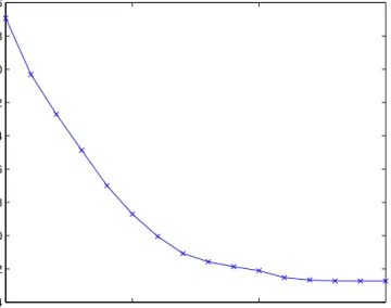
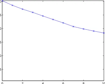
where VH is a constant. If H = 1/2 then the fBm reduces to ordinary Brownian motion. The smaller the values of H the rougher the time series. See figures (1) and (2) for two plots of fBm with H = 0.3 and H = 0.9.

0 200 400 600 800 1000 1200 −8 −6 −4 −2 0 2 4 6 8 10 12 Time Amplitude fBm H=0.3 Figure 1. _{fBm with} _H_{= 0}_.₃ 0 200 400 600 800 1000 1200 0 10 20 30 40 50 60 70 80 90 100 Time Amplitude fBm H=0.9 Figure 2. _{fBm with} _H_{= 0}_.₉

(16)

8. FRACTIONAL BROWNIAN MOTION 15

8.1. Correlation of fBm. One of the most important features of Fractional Brownian Motion is that it has infinite correlation. All the past increments are correlated with the future ones. Now define the increment between 0 and ₋t

as [BH(0)−BH(−t)] and similarly define the increment between 0 and t to be

BH(t)−BH(0). Now using our definition for covariance the, covariance of the increment process is E[(BH(0)−BH(−t))(BH(t)−BH(0)]. We already know that BH(0) = 0 now the correlation function for the increments of fBm is given as follows, ρB(t) = γB(t) var(BH(t)) = E[(BH(0)−BH(−t))(BH(t)−BH(0)] E[BH(t)2] . (2.34) This simplifies to ρB(t) = E[₋BH(−t)BH(t)] E[BH(t)2] . (2.35)

In order to obtain a simpler expression for ρB(t) we carry out the following manipulation

E[(BH(t)−EH(−t))2] =E[BH(t)2] +E[BH(−t)2]−2E[BH(t)BH(−t)]. (2.36) Using the properties of fBm we can express the above equation as:

|t₋(₋t)_|2H ₌_|_t_|2H ₊_|_t_|2H ₋₂_E_[_B

H(t)BH(−t)] (2.37)

|2t_|2H = 2_|t_|2H ₋2E[BH(t)BH(−t)]. (2.38) Now rearranging and makingE[₋BH(t)BH(−t)] the subject we have that

E[₋BH(t)BH(−t)] = (22H

−₁

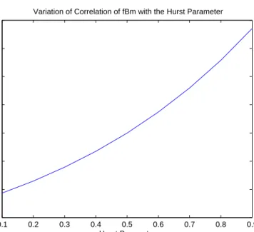
−1)_|t_|2H. (2.39) Now substituting (2.39) into (2.35) we obtain the following expression for the correlation. ρB(t) = E[−BH(−t)BH(t)] E[BH(t)2] = (2 2H−₁ −1)_|t_|2H VH|t|2H = (2 2H−₁ −1) VH (2.40) From the above equation we can see that the correlation of fBm is determined by one parameter and is independent of time. Figure (3) shows the variation of

ρB(t) as the Hurst parameter,H changes. (1) Case 1 when H = 0

ρB(t) = 0 the process is uncorrelated.

(2) Case 2 when H >0.5

ρB(t)>0

This means that the process will consistently behave is a similar manner in the future as it has done in the past.

(17)

0.1 0.2 0.3 0.4 0.5 0.6 0.7 0.8 0.9 −0.6 −0.4 −0.2 0 0.2 0.4 0.6 0.8

Variation of Correlation of fBm with the Hurst Parameter

Hurst Parameter

p(t)

Figure 3. _{Variation of Correlation of fBm with the Hurst Parameter}

(3) Case 3 when H <0.5

ρB(t)<0

This implies that an increasing trend in the past implies a decreasing trend in future.

We have seen that the Hurst parameter, H, effects the correlation of a fBm process and how it changes. Therefore modeling H becomes a very important part of understanding a time series.

Fractional Brownian Motion is said to be a monofractal process. This means that the process only has one fractal dimension associated with it.

(18)

CHAPTER 3

Binomial Multiplicative Cascades

This chapter was based on [1] chapter 3.

A multiplicative cascade is generated by dividing a set up into different parts and to each a measure is assigned. This process then continues and the set gets split in smaller individual parts and at each iteration the initial measure gets distributed. At each iteration the set gets divided into equal parts and each part gets assigned a fraction of the total measure, by multiplying the total measure by a fraction. In order to model real world situations we change the multiplier at each section.

In order to use multiplicative cascades to model time series we divide the unit interval into two parts and assign the fraction of total measure to each part. The measure is divided by multiplying it by a random number from a given distribution. We assume that the original measure is preserved at all stages of the process. In order to divide the measure we multiply the left half of the interval by p and the right half by 1₋p where 0< p <1.

We now illustrate how the multiplicative cascades works. We first denoted the unit interval,[0,1] by I0. Let µbe the function which determines the measure on a specific interval. Therefore µ(I0) = 1 because the measure on the unit interval must be one. The interval is divided into two setsI0,0 andI0,1. WhereI0,0 is from the interval [0,1/2] and I0,1 is from the interval [1/2,1]. The measure allocated to the first interval is µ0 = p and the measure given to the second interval is

µ1 = 1−p. This therefore means that the initial measure is not lost since both

m0 and m1 sum to give one. In the next iteration of the cascade each of the subintervals, I0,0 and I0,1 are split into two. Therefore we have four sets namely

I0,00, I0,01, I0,10, I0,11 over which the original measure is preserved so that:

µ(I0,00) +µ(I0,01) +µ(I0,10) +µ(I0,11) =p2+p(1₋p) + (1₋p)p+ (1₋p)(1₋p) = 1 For each stage of the process the total measure is preserved. At thekth stage of the binomial multiplicative cascade the intervals are defined as follows:

[i2−_k

,(i+ 1)2−_k

] wherei= 0, . . . ,2k₋1.

The measure of one such interval,Ik is given by

µ(Ik) = Πk_i=1mβi =m n0 0 mn 1 1 17

(19)

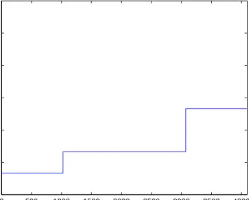
where n1 +n0 = k and they are number of times m1 and m0 are multiplied. Examples of the binomial cascade at different stages are given in figures (1), (2), (3), (4) and (5). 0 500 1000 1500 2000 2500 3000 3500 4000 0 1 2 3 4 5 6

BINOMIAL CASCADE, LEVEL 1

Number of Intervals

Value

Figure 1. _{Binomial Cascade at Level 1}

0 500 1000 1500 2000 2500 3000 3500 4000 0 1 2 3 4 5 6

Value

(20)

3. BINOMIAL MULTIPLICATIVE CASCADES 19 0 500 1000 1500 2000 2500 3000 3500 4000 0 0.2 0.4 0.6 0.8 1 1.2 1.4 1.6 1.8 2

Value

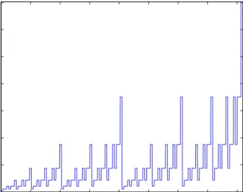
0 500 1000 1500 2000 2500 3000 3500 4000 0 0.05 0.1 0.15 0.2 0.25 0.3 0.35

Value

To observe the scaling property of the binomial cascade we take a point, x

near the origin in our unit interval. The measure of the interval at thekth stage is:

µ([0,2−_k

]) =mk₀ = (2−_k

)ν0

(21)

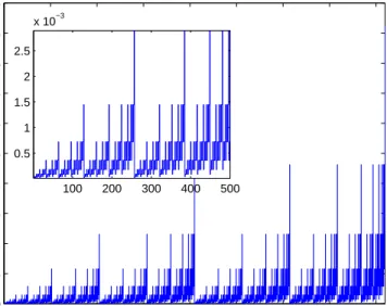
0 500 1000 1500 2000 2500 3000 3500 4000 0 0.005 0.01 0.015 0.02 0.025 0.03 0.035 0.04 0.045 0.05

Number of Intervals Value 100 200 300 400 500 0.5 1 1.5 2 2.5 x 10−3

whereν0 =−log2m0. This means that the measure near to zero has the following scaling property

µ([0, ])_∼α.

Now dividing both sides of the above equation by we see the density has the scaling property: µ([0, ]) ∼α−₁ .

Therefore the density tends to either zero or _∞ provided that α ₆= 1.

This has shown the measure of the neighbourhood of a point arbitatrly close to 0 scales goverened by a power law in the limit as _→0. The scaling exponent

α is also called the H¨older exponent and is a measure of the singularity strength. It is defined as follows

α(x0) = lim →0

logµ(Bx0())

log ,

whereBx0 is the ball of points which are no further thanaway from x0, defined

as

Bx0() ={x:|x−x0|< }.

For the kth interval whose size is 2−_k

the above equation can be simplified to

α(Ik) = log₂µ(Ik) log2(2−k) = log2[m n0 0 mn 1 1 ] log2(2−k) (3.1) = n0 k log2m0− n1 k log2m1. (3.2)

(22)

3. BINOMIAL MULTIPLICATIVE CASCADES 21

We can now simplify the above expression to by letting ₋log₂m0 = ν0 and

−log₂m1 =ν1 to obtain: α(Ik) = n0 k ν0+ n1 k ν1. (3.3) Now let φ= n0

k and we can rewrite (3.3) as

α =φν0+ (1−φ)ν1.

Finally we can takeν0 =αmin and ν1 =αmax which gives:

α=φαmin+ (1−φ)αmax. (3.4) This shows thatα the H¨older exponent is only a function of φ.

The cascade can be characterised using a multifractal spectrum. The multi-fractal sprectrum is the plot of a functionf(α) againstα. We derive the equation for the f(α) for the binomial multiplicative cascade by defining Nk(α) which is the number of intervals with length 2−_k

and H¨older exponent α. We have shown earlier that α could be expressed as a function of just φ. Therefore the number of intervals with H¨older exponentα is the same as the number of ways of distrib-utingn0 =φk zeros ink positions. We can write this as a binomial coefficient as follows: Nk(α) = k φk . (3.5)

Now we can use the following relationships:

k φk = k! (φk)!(k₋zk)!, (3.6) k! =√2πk k e k . (3.7)

Now putting these into (3.5) we obtain

Nk(α) = √ 2πk k_ek √ 2πkφ kφ_ekp 2π(k₋φk) k−_φk e k−kφ (3.8) ≈ [φ φ₍₁₋_φ₎1−φ ]−k p φk(1₋φ) . (3.9)

Now consider the case where φ is small and close to zero and k is much larger than one. The above equation simplifies to

[φφ(1₋φ)1−φ

]−k .

Now define a function h(φ) as follows:

h(φ) =₋log₂[φφ(1₋φ)1−_φ

], (3.10)

(23)

Therefore we can write Nk(α) as:

Nk(α)_∼[2−_k

]−_h(φ)

. (3.12)

Now we make this a function of α. We can rewrite (3.4) as follows

φ= αmax−α αmax−αmin . (3.13)

Now we substitute φ into h(φ) and use 1₋φ = α₋αmin αmax−αmin , to obtain: f(α) = ₋ αmax−α αmax−αmin log₂ αmax−α αmax−αmin (3.14) − α₋αmin αmax−αmin log₂ α₋αmin αmax−αmin . (3.15) If we now expand the above equation around α0 = (αmax +αmin)/2 and use the Talyor expansion of log(x) and for (α₋α0)1 we get:

f(α) = 1₋ 2 log 2 α₋α0 αmax−αmin 2 . (3.16)

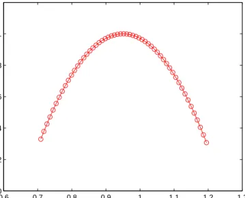
We have calculated the multifractal spectrum for the binomial cascade. The curve f(α) allows us to estimate the fractal dimension of the set of intervals whose H¨older exponent equal to α. It is important to notice that the curve has its maximum atα =α0 and when α=α0 then f(α) = 1. Also f(α) is symeteric with respect to α0. In order to calculate f(α) is practice we use the method of moments.

(24)

3. BINOMIAL MULTIPLICATIVE CASCADES 23 0.6 0.7 0.8 0.9 1 1.1 1.2 1.3 0 0.2 0.4 0.6 0.8 1 α f( α ) Multifractal Spectrum

(25)

(26)

CHAPTER 4

Multinomial Multiplicative Cascades

This chapter was based on [1] chapter 3.

In order to generalise the binomial cascade instead of dividing the unit interval up into two parts we divide it up intobparts in a similar way. As for the binomial case the total measure will be conserved after each iteration. Let us define akth stage cascade where the multipliers arem0, m1, . . . , mb−₁. At thekth stage there

willbk _{intervals of length}_b−k

. The measure at a random instant can be expressed as: µ(I_bk) =mn0 0 m n1 1 . . . m nb−1 b−1 = Π b−₁ i=0m ni i = Πb −₁ i=0m φik i , (4.1)

where we define ni are the number of times which the ith multiplier is repeated in that particular interval of the cascade. φik is the percentage number of times theith multiplier is repeated. Now we have that the interval is Ik

b and the length of this interval is b−_k

. Therefore using (3.3) we can define α for a multinomial cascade α= logbµ(I k b) log_bb−k = log_b[Πb−₁ i=0m φik i ] −k . (4.2)

Which we can simplify to give

α=₋ b−1 X

i=1

φilogbmi (4.3)

Thereforeα depends on the percentage number of times a multiplier is repeated in a cascade.

In order to define the multifractal spectrum we define Nk(α) which is the number of intervals which have α as their H¨older exponent. At the kth stage of the cascade there are k! ways in which the multipliers for every point can be arranged. The multipliers can be arranged in ni! ways where i= 0,_{· · · −}1. The expression Πb−₁

i=0ni is the number of multipliers which have the same percentage of multipliers present for the measure. Therefore we can write Nk(α) as:

Nk(α) = k! Πb−₁

i=0ni!

. (4.4)

If we now take logs of both sides we have logNk(α) = logk!− b−₁ X i=0 logni!. (4.5) 25

(27)

We can simplify (4.5) using Stirling approximation given below: logn! =nlogn₋n (4.6) =_⇒ logNk(α) = klogk−k− b−1 X i=0 nilogni− b−1 X i=0 ni (4.7) =_⇒ logNk(α) = klogk₋ b−1 X i=0 nilogni (4.8) since Pb−₁

i=0ni = k. Now use the substitution ni =φik in the above equation to obtain: log_bNk(α) =klog_bk₋ b−₁ X i=0 log_b(φik)φik (4.9) =klogbk−k b−₁ X i=0 φilogbφi−klogbk b−₁ X i=0 φi (4.10) =₋k b−₁ X i=0 φilogbφi. (4.11)

If we remove the logs in the above equation we can see that

Nk(α) = (b−_k

) bi=0−1φilogbφi_. _(4.12)

To simplify this equation we will write

δ=₋ b−1 X

i=0

φilogbφi. This means that (4.12) becomes

Nk(α) = (b−k

)−δ

. (4.13)

The range of value which δ can take are called the scaling parameters.

The choice of possible functions for f(α) are governed by the following equa-tions: b−₁ X i=0 φi = 1 and (4.14) − b−₁ X i=0 φilogbmi =α. (4.15) We need to find a φi which maximises

−

b−₁ X

i=0

(28)

4. MULTINOMIAL MULTIPLICATIVE CASCADES 27

with respect to the equations (4.14). This problem is solved using Lagrange multipliers. We first define G as follows

G=₋ b−₁ X i=0 φilogbφi+q " α+ b−₁ X i=0 φilogbmi # .

Differentiating G with respect to φi and setting the equation equal to zero to obtain the critical points we have:

∂G ∂φi

=₋[log_bφi+ 1] +qlogbmi = 0 (4.16) =_⇒ log_bφi =−1 +qlogbmi (4.17) =_⇒ φi =b[−1+qlogbmi]. (4.18) We now impose the condition

b−₁ X i=0 φi = 1 in (4.18) to obtain: b−1 X i=0 b[−1+qlog_bm_i] = 1 (4.19) =_⇒ b−₁ X i=0 mq_i =b. (4.20)

We now have an expression forb which we put back into (4.18) and obtain three expressions φi = b−₁ X i=0 mq_i ![−1+qlogbmi] (4.21) = Pb−₁ i=0m q i qlogbmi Pb−1 i=0m q i (4.22) = m q i Pb−1 i=0m q i . (4.23)

Now we can substitute this value forφi into (4.3) to find an expression forα

α=₋ b−₁ X i=0 mq_i Pb−₁ i=0m q i ! log_bmi. (4.24)

(29)

Now combining the previous equations we obtain an expression forf(α) f(α) =₋ b−1 X i=0 mq_i Pb−₁ i=0m q i ! log_b m q i Pb−₁ i=0m q i ! . (4.25)

The expression for

b−1 X

i=0

mq_i

is like a partition function. We define a new quantity

τ(q) =₋logb

X

i

mq_i.

We can write α in terms of a partial derivative of the function τ(q) as

α = ∂τ(q)

∂q .

In the same way we rewrite the expression for f(α) as

f(α) =q∂τ(q)

∂q −τ(q) =qα−τ(q). (4.26)

Equation (4.26) is known as the Legendre transform. The above transform can be made possible for all q as follows:

f(α) = min

(30)

CHAPTER 5

Estimating the Multifractal Spectrum in Practice

This chapte was based on [1].

In practice it is diffucult to find the scaling exponent, or the partition function,

τ(q). Therefore we have to find a suitable way to estimate the scaling exponent. The method we will use is called the method of moments. The idea behind the method of moments is to use the fact that the multifractal spectrum gives a measure of the distribution ofαthe H¨older exponent. Therefore we can estimate the multifractal spectrum by studying the H¨older exponents. We chose a partition function such that it illustrates the singularities in the cascade. We first obtain an estimate forτ(q) for all values ofq. This is then used to obtain an estimate for

f(α) which we then use to plot the multifractal spectrum. The partition function is defined as: Xq() = N() X i=1 (µi)q (5.1)

where µi is the measure of Bi()N()i=1 and q ∈R. The way in which the measure for the cascade is distributed in the general case is given by:

µi =αi. Simply replacing this relation in (5.1) we obtain:

Xq() = N()

X

i=1

(αi₎q_. _(5.2)

Now define N(α) to be the number of boxes with size and N(α)dα is the number of boxes of size which have H¨older exponent which lies in the interval (α, alpha+dα). The boxes of this type each adds N(α)(α₎q_dα _to _X_q(_{). Now} the contribution that anyα would add to Xq() is given by

Xq() =

Z

N(α)(α)qdα (5.3) Now note that we can generalise (3.12) to give

N(α)_∼−_f(α) .

Substituting into (5.3) gives

Xq() =

Z

αq−_f(α)

dα. (5.4)

(31)

If take the limit as_→0 the largest part of the integral would be from the values of α which minimise,

αq₋f(α).

In order to minimise the above equation we simply differentiate the above equa-tion with respect to α and set it equal to zero

d

dα(αq−f(α)) = 0. (5.5)

Now for our estimate we will keep only the largest contribution to the integral and discard the rest. Then we can write the formula for τ(q) as,

τ(q) = min

α (qα−f(α)). (5.6) We also have the other relation

Xq()_∼τ(q).

We can take logs of the above equation and use it to estimate τ(q):

logXq()_∼τ(q) log. (5.7) We can obtain a relationship for f(α) which is given below:

f(α) = min

(32)

CHAPTER 6

Methods for Measuring Statistical Properties in Data

This chapter was based on [1], [9], [6] and [10].

1. Variance-Time Plots

One common method used for measuring the degree of self-similarity in the data is variance-time plot. It enables us to also give a fairly crude estimate for the Hurst parameter. We can characterise LRD dependence and self-similarity in term of an aggregated process defined as:

X(m)₍_n_{) :=} 1 m km X i=(k−_1)m+1 X(i). (6.1)

Where the time series [X(t) :t = 1, . . . N/m] is divided in blocks of lengthm and aggregated as above.

The sample variance is defined as: ˆ var(X(m)₍_n_{)) =} 1 (N/m)₋1 N/m X n=1 (X(m)(n)₋X) whereX is the sample mean.

The process is called second order self-similar or exact self-similar process if var(X(n)) = m2−2H

var(X(m)(n)).

In this case the log-log plot, variance-time plot, of var(X(m)₍_n_{)) against} _m _is strictly linear ignoring small values ofm. The slope of the line of an exact self-similar process on a log-log plot is

2₋2H.

Where H is the Hurst parameter. Therefore for a self-similar process we can estimate its Hurst parameter by plotting a least squares line on the variance-time plot and measuring its gradient ˆβ. The Hurst parameter is then given by

ˆ

β = 2₋2H (6.2)

=_⇒ H = 1

2(2−βˆ). (6.3)

A value of ˆβ between -1 and 0 indicates a degree of self-similarity and LRD.

(33)

2. Method of Absolute Moments

There are many different definitions of a process being self-similar. One defin-ition investigates self-similarity using absolute moments. Define theqth moment of the aggregated process X(m) _{to be:}

µ(m)(q) := E_|X(m)_|q. Define X(m) _{as follows:} X(m)= 1 m m X i=1 X(i).

Therefore the qth moment is defined as:

µ(m)(q) :=E_|1 m m X i=1 X(i)_|q.

If the processXis self-similar thenµ(q)_{is proportional to}_mβ(q)_{. This is equivalent} to saying the logs of both sides have a linear relationship:

logµ(m)(q) =β(q) log(m) +C(q). (6.4) From self similarity we also require that β(q) is linear with respect to q. Since we have that X=d_m1−_H

X(m) _{we have the following equation:}

β(q) = q(H₋1). (6.5) Therefore we have another definition for self similarity namely that the moments must satisfy (6.4) and β(q) must satisfy (6.5).

The previous definition for self-similarity can be generalised to multifractal processes. Therefore for a non negative process X(t) it is multifractal if the logs of absolute moments scale linearly with respect to the logs of aggregation levels m. If a multifractal can take both positive and negative values it is called signed multifractal. A signed multifractal process does not have to have scaling exponent β(q) linear with respect toq. Therefore a signed multifractal process is a generalised self similar process. In order for us to be able to determine whether a process is multifractal self-similar or signed multifractal we need to examine the higher moments of the process.

(1) IfX is a positive stationary time series, then X or X₋EX can not be self similar.

(2) However, the sequence X₋EXmay asymptotically self-similar.

(3) IfX is self-similar with meanEX then the following relationship holds.

EX =m1−_H

EX(m) =m1−_H EX.

(34)

2. METHOD OF ABSOLUTE MOMENTS 33

(4) If X is asymptotically self-similar then

EX _∼m1−H EX

for large m.

(5) If the process has zero mean it could be multifractal.

The goal when using moments is to determine whether X orX₋EX is a self similar, multifractal or signed multifractal process. We estimate theqth moment of X,µ(m)₍_q_{) we use the} _q_{th sample absolute moment.}

ˆ µ(m)₍_q_{) =} 1 N/m N/m X n=1 |X(m)(n)_|q_. _(6.6) If the log of the sample absolute moments is linear with respect to the log ofm. Then a multifractal model is suitable to model X. In practice we only plot the moments forq = 1,2,3,4 because higher moments are not well behaved.

(35)

(36)

CHAPTER 7

Analysis of Sample Data

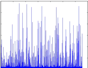
The data we will use to fit our model is a set of Ethernet LAN traffic measure-ments. It was collected on an internal Bellcore Ethernet LAN during a normal traffic hour in August 1989. The data represents the number of Ethernet packets at the 10 millisecond time scale. We will apply variance-time plot to observe the self-similarity properties of the data. We will also calculate the absolute moments of the data and the absolute moments minus the sample means of the time series. To investigate whether or not the time is suitable to be modelled by a multifrac-tal model we will also plot a multifracmultifrac-tal spectrum by first plotting the partition function with varying q. Figure (1) is the raw time series data from Bellcore.

0 0.5 1 1.5 2 2.5 3 3.5 x 104 0 0.02 0.04 0.06 0.08 0.1 0.12

Bellcore Data Set

Packet Group Number

Interarrival Time

Figure 1. _{Bellcore Ethernet Packet Data}

From figure (1) above we can see that most of the interarrival times are below 0.01. However the challenge when modelling the bellcore data is to model the irregular burstiness which we observe in the plot. This property is something that a model such as fBm struggles to model because of its underlying Gaussian assumptions. In fBm the Hurst parameter is a constant and therefore it struggles to model physical data for which the self-similarity varies with time. Therefore a

(37)

multifractal model is more appropriate. To examine self-similarity properties of the data we take a variance-time plot see figure (2).

0 5 10 15 −32 −30 −28 −26 −24 −22 −20 −18 −16 −14 log 2(m) log 2 (var(X m(n)))

Variance−Time Plot of the Bellcore Data

Figure 2. _{Variance-Time Plot of the Bellcore Data}

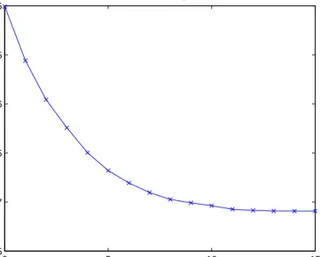
We can see from figure (2) that the plot is slightly linear. This suggests a degree of self-similarity. The gradient of the least squares line is -0.61. Which gives a Hurst parameter estimate of 0.7. This suggests that there is degree of self simlilarity present in the data. Now to investigate whether the data is a multifractal process we plot the log absolute moments against the aggregated time in figures (3), (4),(5) and (6).

The log moment plots, figures (3), (4),(5) and (6), clearly do not scale linearly with respect to the log of the aggregation value m. Therefore to investigate whether this process can be modeled with a multifractal modeled we need to examine whether the log moment plot with the mean subtracted, scale linearly. If it does this suffests the data is suitable to be modelled by the multifractal model we will propose. The log moment plots with subtracted means is given below are shown in figures (7), (8),(9) and (10).

Now with the means subtracted from the series the logarithm of the moments now scales linearly with respect to the log ofmthe aggregation level. From figures (7), (8),(9) and (10) we can see that the moments scale linearly with respect to

m. This confirms that the process can be suitably modeled by a multifractal process.

We now examine the partition function to investigate the multifractal nature of the data. If the process has multifractal properties then the partition equation

(38)

7. ANALYSIS OF SAMPLE DATA 37 0 5 10 15 −17.5 −17 −16.5 −16 −15.5 −15 Moments for q=2 log 2(m) log 2 (Moments)

Figure 3. _{Plot of the Absolute Moments of the Bellcore Data}

with q = 2 0 5 10 15 −26 −25 −24 −23 −22 −21 −20 −19 Moments for q=3 log 2(m) log 2 (Moments)

with q = 3

will show linearity with respect to log(m). The plot of the partition functions is shown in figure (11).

(39)

0 5 10 15 −36 −34 −32 −30 −28 −26 −24 −22 Moments for q=4 log 2(m) log 2 (Moments)

with q= 4 0 5 10 15 −44 −42 −40 −38 −36 −34 −32 −30 −28 −26 Moments for q=5 log 2(m) log 2 (Moments)

with q= 5

We can clearly see from figure (11) that disregarding small values of log₂(m) the partition functions exhibit lineararity with respect to log₂(m). We now look at the variation of the scaling parameter τ(q) with respect to q in figure (12).

(40)

7. ANALYSIS OF SAMPLE DATA 39 0 2 4 6 8 10 −32 −30 −28 −26 −24 −22 −20 −18 −16

Moments for q=2 with Mean Subtracted

log

2(m)

log

2

(Moments)

Figure 7. _{Plot of the Absolute Moments Minus Sample Means of}

the Bellcore Data with q = 2

0 2 4 6 8 10 −45 −40 −35 −30 −25 −20

log

2(m)

log

2

(Moments)

the Bellcore Data with q = 3

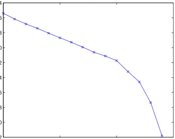
Figure (12) shows that there is a linear relationship and that τ(q) is an in-creasing function. The multifractal nature of the Bellcore is clearly shown in its multifractal spectrum seen in figure (13).

(41)

0 2 4 6 8 10 −65 −60 −55 −50 −45 −40 −35 −30 −25

log

2(m)

log

2

(Moments)

the Bellcore Data with q= 4

0 2 4 6 8 10 −80 −75 −70 −65 −60 −55 −50 −45 −40 −35 −30

log

2(m)

log

2

(Moments)

Figure 10. _{Plot of the Absolute Moments Minus Sample Means}

of the Bellcore Data with q= 4

This is a typical multifractal spectrum and suggests that the Bellcore data is multifractal in nature and can be modelled by a multifractal model. We have seen

(42)

7. ANALYSIS OF SAMPLE DATA 41 0 5 10 15 −40 −20 0 20 40 60 80

Partition Function for Bellcore Data

log

2

(Partition Function)

log

2(m)

Figure 11. _{Partition Functions of the Bellcore Data}

−5 0 5 −8 −6 −4 −2 0 2 4 q τ (q) Variation of τ(q) with q

Figure 12. _{Variation of} _τ₍_q_{) with respect to} _q

that the Bellcore data shows a degree of self-similarity, burstiness and multifractal scaling.

(43)

0.6 0.7 0.8 0.9 1 1.1 1.2 1.3 1.4 0.2 0.3 0.4 0.5 0.6 0.7 0.8 0.9 1 1.1 α f( α )

Multifractal Spectrum of the Bellcore Data

(44)

CHAPTER 8

Multifractal Wavelet Model

This section was based on the paper [8] and chapter 3 in [1].

The multifractal wavelet model was developed by Riedi et al in [8]. It is a multifractal process based on the binomial multiplicative cascade. It is a signal model for positive, stationary, long range dependent data.

The discrete wavelet transform represents a one dimensional random process in a multi scale representation. The random processX(t) is represented in terms of a shifted and dilated versions of the prototype wavelet functionψ(t) and shifted versions of a scaling functionφ(t). The wavelet function and scaling function are defined by the following family of functions:

ψj,k(t) = 2j/2ψ(22t₋k), (8.1)

φj,k(t) = 2j/2φ(2jt₋k), (8.2) form an orthonormal basis for special choices of the wavelet. When they form an orthonormal basis the process can represented as:

X(t) =X k UJ0,kφJ0, k(t) + ∞ X j=J0 X k Wj,kψj,k(t). (8.3) We will use the Haar wavelet family defined as:

φ(x) = ( 1 if 0 _≤t_≤1 0 Otherwise ψ(x) =      1 if 0_≤t _≤0.5 −1 if 0.5_≤t_≤1 0 Otherwise.

Where Wj,k is the wavelet coefficient and Uj,k is the scaling coefficient and they are defined as:

Wj,k = Z X(t)ψj,kdt (8.4) Uj,k = Z X(t)φj,kdt (8.5) The wavelet ψ(t) is centred at time zero and has frequency f0. The wavelet coefficient measures the signal around time 2j_k _{and the frequency 2}j_f_{0. The}

(45)

scaling coefficient Uj,k measures the local mean around the time 2−jk. The index

j is the scale of analysis. The constantJ0 is the coarsest scale of the analysis and as j increases this gives a finer scale and higher resolution of the analysis. The Haar scaling and wavelet functions which the multifractal wavelet model uses is the simplest example of a orthonormal wavelet basis. The scaling function φ(t) for the Haar wavelet defines the scaling coefficients which are nested where the coefficient for coarse scales supports the scaling coefficient for fine scales.

Row j in the scaling coefficient tree contains an approximation of X(t) at resolution 2−_j

.

The wavelet and scaling coefficients of the Haar wavelet are defined by the following recurisive relationship

Uj,k = 2− 1 2[U j+1,2k+Uj+1,2k+1] (8.6) Wj,k = 2 −1 2[U j+1,2k−Uj+1,2k+1]. (8.7) The scaling coefficientsUj,k give the local mean of the signal at different scales and times.

The multifractal wavelet model aims to model a stationary, long range de-pendent, positive signal, c(t). We will use the discrete time increment process

c(n)_[_k_{] to approximate} _c₍_t_{) at the resolution 2}−_n

. This approximation is shown (8.3) where we replace the semi infinite sum from J0 to infinity by a sum over a finite number of scales where j goes from 0 ton and j, n_∈ Z_{+. Without losing} generality we can set the coarsest scale J0 equal to zero. This means that the first sum in (8.3) is the just the term U0,0φ0,0.

It is important the the model is easy to use, gives a fast analysis, the synthesis should match the positive process closely and exhibit LRD. We will now show how it is possible to do this using a Haar wavelet to construction the increment process C(n)_[_k_].

We must ensure that the output of the wavelet model gives a positive process. First we note the the Haar wavelet and scaling coefficients are defined as (8.6). The scaling coeffficients are non negative if and only the signal is greater than or equal to zero. This is true because each Uj,k is equal to a scaled local mean. We can rewrite equations (8.6) as

Uj+1,2k = 2 −1 2(U j,k+Wj,k) (8.8) Uj+1,2k+1 = 2 −1 2(U j,k−Wj,k). (8.9) Therefore since the signal must be positive the wavelet coefficients must satisfy the following condition

|Wj,k| ≤Uj,k. (8.10) We incorporate (8.10) in to a simple multiplicative model for the wavelet coefficients. This is achieved by defining a random variable Aj,k in the range

(46)

1. SYNTHESIS 45

[₋1,1] and defining Wj,k recursively as

Wj,k =Uj,kAj,k. (8.11) Therefore the MWM incorporates the Haar wavelat and the multplicative recur-sion relation (8.11).

1. Synthesis

The MWM is a coarse to fine synthesis which is given by:

(1) We start with j = 0, the coarsest resolution, and compute the corre-sponding scaling coefficient U0,0. This gives us the global mean of the signal.

(2) At scale j we generate the random multipliers Aj,k and use

Wj,k =Uj,kAj,k k= 0, . . . ,2j−1 to compute the wavelet coefficients.

(3) Still at scale j we use Wj,k, Uj,k and the recursion relations below

Uj+1,2k = 2 −1 2(U j,k+Wj,k) (8.12) Uj+1,2k+1 = 2 −1 2(U j,k−Wj,k) (8.13) to calculate the scaling coefficientsUj+1,2kandUj+1,2k+1fork = 0, . . . ,2j− 1.

(4) We repeated steps 2 and 3 until we reach our finest scale j =n

The scaling and wavelet coefficients are generated together therefore we do not need to invert the wavelet transform in order to calcualte the wavelet coeffi-cents. The scaling coefficients obtained at the finest scale are the output process. Therefore we have

C(n)[k] = 2−_n/2

Un,k (8.14)

wherek = 0, . . . ,2n₋_1.

The Haar wavelet’s simplicity allows us to devire direct expressions for the scaling and wavelet coefficients in terms of justU0,0 and the random variableAj,k. In order to do this we define an indexing scheme to relate the coarsest scaleU0,0 to all the finer scales. Letkj be an indexing variable for j >0, which indexes the possible shift of the descendants of U0,0 at a finer scale j. The shift of a scaling coefficient given bykj can be related to the shift of the scaling coefficient’s direct descendants, kj+1, by

kj+1 = 2kj+k

0

(47)

Where k0

j = 0 is the left descendant and k

0

j = 1 is the right descendant. Using (8.15) we can expresskj as a binary expansion in terms ofk

0 i wherei= 0, . . . , j−1 kj = j−1 X i=0 ki2j−1−i . (8.16)

The picture below gives an illustrations of how the indexing work from a coarse scale to a finer one.

U0,0 U1,0 U1,1 U2,0 U2,1 U2,2 U2,3 k0 0 = 0 @ @ @ @ @ @ @ R k0 0 = 1 k0 1 = 0 A A A A A AU k0 1 = 1 k0 1 = 0 A A A A A AU k0 1 = 1

Now using this indexing variable we can define the wavelet and scaling coef-ficients in closed-form expressions.

Definition _8.1. _{The wavelet and scaling coefficient of the Haar wavelet can}

be defined in terms of the random variable Aj,k on[−1,1]by the general relations:

Uj,kj = 2 −j 2U 0,0 j−₁ Y i=0 [1 + (₋1)k0iA i,ki] (8.17) Wj,kj = 2 −j 2A j,kjU0,0 j−₁ Y i=0 [1 + (₋1)k0iA i,ki]. (8.18) 2. Properties of MWM

The Haar wavelet coefficients have the property that they are identically dis-tributed for each scale and that E[Wj,k] = 0. To model these properties in our model we impose the following condition on the random variables Aj,k.

(48)

2. PROPERTIES OF MWM 47

(1) The multipliers are Aj,k where k = 0,1, . . . ,2j−1 are identically distrib-uted in accordance to the random variable A(j) ∈[−1,1].

(2) Aj,k are symmetrically distributed with respect to zero. (3) Aj,k are independent ofU0,0 and Al,k for l > k.

Now using the above conditions for Aj,k, the equations (8.17) and setting

j =n and k =kn we obtain C(n)[k] = 2−_n U0,0 n−₁ Y i=0 (1 + (₋1)k0iA i,ki) (8.19) =d2−_n U0,0 n−₁ Y i=0 (1 +A(j)). (8.20)

Therefore we can say that C(n)_[_k_{] is a first order stationary process and that is} identically distributed.

Now given our independence assumption earlier the qth _{moment of} _C(n)_[_k_{] is} given by E[C(n)[k]q] = E[U_0,0q ] n−₁ Y j=0 E 1 +A(j) 2 q . (8.21)

We will assume that the Aj,k random variables that are independent, as a consequence the wavelet coefficients will be uncorrelated. The wavelet coefficients are not correlated because if we were in calculating the correlation; all terms of the formE[Aj,k] would be zero becauseE[Aj,k] = 0. There is correlation however for higher order structures which maintains the models positive output.

Finally we must make it possible for the model to be able to synthesise data. This is achieved by defining pfds forU0,0 and the multipliers, A(j), at each scale. The pdfs are chosen for theA(j) variabels such that we can control the wavelet scaling behaviour using (8.17). This scaling behaviour allows us to control the correlations in the data.

If we consider the Karhunen-Loeve transform. It has been shown that the wavelet transform approximately decorrelates LRD signals and 1/f processes. Using this idea we can approximately control the correlation behaviour by chang-ing the second order moments of the wavelet coefficients at each scale.

We control the correlation behaviour by fixing the energy at the coarsest scale,

U0,0. The ratio of energies for other scales is set as follows:

νj =

var(Wj−1,k)

(49)

for 0 _≤ j < n. Now using the equation (8.18) we can calculate the ratios of energies for the MWM as follows:

νj = E[W2 j−_1,k] E[W2 j,k] (8.22) = 2E[A 2 (j−₁₎]E[U 2 j−1,k] E[A2 (j)]E[(1 +A(j−1))2]E[U_j2−_1,k] (8.23) = 2 E[A 2 (j−₁₎] E[A2 (j)](1 +E[A2(j−₁₎]) . (8.24)

In order to match the variance decay for any scale, we can solve (8.24) recur-sively for E[A2

(j)] in terms of νj and E[A(j2−₁₎] for j = 1, . . . , n−1. The initial

point for the coarest scale is given by:

E[A2₍₀₎] = E[W 2 0,0] E[U2 0,0] . (8.25)

Now we look at the pdf which we will use for the multipliersAj. The distribu-tion we use is called the symmetric beta distribudistribu-tion. A β(p, p) random variable,

Aj, is symmetrically distributed over the interval (−1,1) and the probability density function is defined as

gA(a) =

(1 +a)p−1

(1₋a)p−1 B(p, p)22p−₁ .

Where B(p, p) is the beta function and p >0 is called the shape factor. B(p, p) is defined as:

B(α, β) = Γ(α)Γ(β)

Γ(α+β). (8.26)

Where α, β >0 and Γ is the Gamma function defined as: Γ(δ) = Z ∞ 0 yδ−₁ e−_y dy (8.27)

with δ is a positive integer.

For large values of p the beta distribution is approximately Gaussian. The variance is defined as

var(A) =E[A2] = 1

2p+ 1. (8.28)

The choice of how to choose the p values correctly to give the desired scaling behaviour parameterised by νj is done using (8.24) and (8.28). This gives us the

(50)

3. BETA MULTIFRACTAL WAVELET MODEL ANALYSIS OF THE BELLCORE DATA 49 following relation: νj = 2 E[A2 (j−₁₎] E[A2 (j)](1 +E[A2(j−1)]) (8.29) = 2 2pj+1 1 2pj+1[1 + 1 2pj+1] (8.30) pj = νj 2[1 +p(j−1)]− 1 2. (8.31)

When we use the beta distribution for the Aj multpliers we call the model

βMWM.

3. Beta Multifractal Wavelet Model Analysis of the Bellcore Data We now turn our attention to using the βMWM to synthesise the Bellcore data. This will test the model’s ability to take in to consideration the long range dependence and the multifractal scaling present in the data. We apply the algorithm for synthesising the data for the βMWM model. The Haar wavelet transform of the Bellcore is computed. The algorithm uses results from the preivous section in order to adjust the variances of the wavelet coefficients to match the variances and correlation in the Bellcore Data. To obtain a good estimate for the Bellcore data we perform the synthesis for the 12 finest scales and concatenate 15 of the synthetic traces of the Bellcore data. In figure (1) we plot the synthetic trace of the trained βMWM model.

0 0.5 1 1.5 2 2.5 3 3.5 x 104 0 0.01 0.02 0.03 0.04 0.05 0.06 0.07 0.08 0.09 0.1

The Synthetic Trace of βMWM for the Bellcore Data

Packet Group Number

Interarrival Time

(51)

The synthetic trace,(1). shows that theβMWM model mimics the burstiness in the Bellcore data. It also looks like there is multifractal scaling and a degree of self-similarity present in the synthetic trace. To investigate the self-similarity properties of the synthesised data we compute a variance-time plot, figure (2).

0 5 10 15 −28 −26 −24 −22 −20 −18 −16 −14

Variance−Time Plot of the βMWM Synthetic Trace

log 2(m) log 2 (Var(X m(n))

Figure 2. _{Variance-Time Plot of the Synthesised Data}

The variance-time plot (2) shows linearity this suggests that the process has a degree of self-similarity and LRD. After plotting a least squares regression on the variance time plot we obtain a estimate for the gradient, ˆβ = ₋0.62. This estimate is in the required range, 0 >β >ˆ ₋1 to suggest self-similarity and LRD. This gives a value of ˆH = 0.7. This shows that the MWM model has successfully modelled the long range dependence in the Bellcore data. To investigate the multifractal properties of the synthetic data we will now plot the log of the partition function against varying values of log₂(m) in figure (3).

Disregarding the values of 0 to 4 of log₂(m) the partition functions in figure (3) are linear with respect to log₂(m). This linearity suggests that there is mul-tifractal properties present in the synthesised data. Therefore the βMWM has successfully model the multifractal nature of the data.

Figure (4) is a plot of the scaling parameterτ(q) against q=₋5. . .5. Figure (4) shows that the scaling parameter τ(q) is an increasing function with respect to q. Figure (5) is a plot of the multifractal spectrum of the data.

Figure (5) is a typical multifractal spectrum. This clearly shows that the multifractal wavelet model has successfully mimicked the multifractal properties in the Bellcore data.

(52)

3. BETA MULTIFRACTAL WAVELET MODEL ANALYSIS OF THE BELLCORE DATA 51 0 5 10 15 −50 0 50 100 150 200

Partition Function Plot for the βMWM Synthetic Trace

log

2(m)

log

2

(Partition Function)

Figure 3. _{Plot of the Partition Functions for the Synthesised Data}

−5 0 5 −10 −8 −6 −4 −2 0 2 4 q τ (q)

Variation of τ(q) with q for the βMWM Synthetic Trace

(53)

0.6 0.8 1 1.2 1.4 1.6 0 0.2 0.4 0.6 0.8 1 α f( α )

Multifractal Spectrum of βMWM Synthetic Trace

(54)

CHAPTER 9

Erramili Map

This section is based on [3] and [4].

Until the 1990s it was thought that the computer packet traffic exhibited only Possion characteristics namely that packet traffic was memoryless. In the early 1990s the property of long range dependence was discovered in network traffic. The major modelling task became to model this long range dependence. The biggest difficultly in modelling long range dependent network traffic is to incorporate the burstiness which is present in long range dependent traffic.

One model suggested in the 1994 by Erramilli is a one dimensional itterative chaotic map. This model aims to mimic this long range dependence and bursti-ness present in network traffic. The Erramilli model has caused interest because it it is a simple dynamical system and it was thought that it is not possible to model long range dependent data using a dynamical system. The model is defined as the mapf(x): f(x) = ( x+1−d dm1x m1 if 0_≤x < d x₋₍₁−_d)dm2(1−x) m2 if d ≤x_≤1.

Where d, m1, m2 are parameters with m1, m2 ∈(3/2,2) and d∈(0,1). A plot of the map is shown in figure (1):

The line at x= 0.5 is a asymptote. The line y=xis also an asymptote. The map has two non-hyperbolic unstable fixed points at zero and one.

The map itself does not exhibit long range dependence it is the binary se-quence which we use to model the network traffic and long range dependence. The idea is that the right half of the map,d_≤x <1 is considered ON and the left half 0_≤x < d is OFF. It we start with a point x0 in in OFF interval 0≤x < d and if the point f(x0) is in the OFF interval a zero is emmited atternatively if

f(x0) is in the ON interval a one is emmited. This is called the indicator function and is defined as

g(x) =

(

0 if 0 _≤x < d

1 if d_≤x_≤1.

For a random starting point x0 we follow its orbit and record the sequence the value ofg after each iteration. A typical sequence S of lengthN is given by:

S = (g(x0), g(f(x0)), g(f2(x0)), . . . , g(fN−₂

(x0)), g(fN−₁

(x0))).