Risk Classi…cation for Claim Counts and Losses Using
Regression Models for Location, Scale and Shape
George Tzougas
Department of Statistics, School of Mathematical Sciences, University College Cork, Ireland
Department of Statistics, Athens University of Economics and Business Spyridon Vrontos
Department of Mathematical Sciences, University of Essex Nicholas Frangos
Department of Statistics, Athens University of Economics and Business November 30, 2015
Abstract
This paper presents and compares di¤erent risk classi…cation models for the frequency and severity of claims employing regression models for location, scale and shape. The di¤erences between these models are analyzed through the mean and the variance of the annual number of claims and the costs of claims of the insureds, who belong to di¤erent risk classes and interesting results about claiming behaviour are obtained. Furthermore, the resulting a priori premiums rates are calculated via the expected value and standard deviation principles with independence between the claim frequency and severity components assumed.
Keywords: Claim frequency; Claim severity; Regression Models for Location, Scale and Shape; A priori risk classi…cation; Expected value premium calculation principle; Standard deviation premium calculation principle.
Acknowledgements: The authors would like to thank the Editor in Chief and the referees for their constructive comments and suggestions.
Athens University of Economics and Business, 76 Patission Str., 104 34, Athens, Greece, Tel: +302108203579, Email: [email protected]
1
Introduction
The idea behind a priori risk classi…cation is to split an insurance portfolio into classes that consist of risks with all policyholders belonging to the same class paying the same premium. In view of the economic importance of motor third party liability (MTPL) insurance in developed countries, actuaries have made many attempts to …nd a probabilistic model for the distribution of the number and costs of claims reported by policyholders.
Recent actuarial literature research assumes that the risks can be rated a priori using gener-alized linear models, GLM (see Nelder and Wedderburn, 1972) and genergener-alized additive models, GAM (see Hastie and Tibshirani, 1990). For motor insurance, typical response variables in these regression models are the number of claims (or claim frequency) and its corresponding severity. References for a priori risk classi…cation include, for example, Dionne and Vanasse (1989, 1992), Dean et al. (1989), Denuit and Lang (2004), Yip and Yau (2005), and Boucher et al. (2007). Speci…cally, Dionne and Vanasse used a Negative Binomial Type I regression model. Dean et al. used a Poisson-Inverse Gaussian regression model. Denuit and Lang used generalized additive models. Yip and Yau presented several parametric Zero-In‡ated count distributions and Boucher et al. presented a comparison of various Zero-In‡ated Mixed Poisson and Hurdle Models. Also, a review of actuarial models for risk classi…cation and insurance ratemaking can be found in Denuit et al. (2007).
The models brie‡y described above assume that only the mean is modelled as a function of risk factors. However, any model for the mean in terms of a priori rating variables indirectly yields a model for scale and/or shape. Also, even if the mean is the most commonly used measure of the expected claim frequency and of the expected claim severity it does not provide a good description of a distribution’s scale and shape. Speci…cally, the scale and shape parameters are not adequately described due to the unobserved heterogeneity changes with explanatory variables. In this study, we extend this setup by assuming that all the parameters of the claim frequency/severity distributions can be modelled as functions of explanatory variables with parametric linear functional forms. Joint modelling of all the parameters in terms of covariates improves rate making and estimation of the scale and shape of the claim frequency/ severity distributions. Speci…cally, in light of a priori ratemaking there is a substantial bene…t in this approach since by modelling all the parameters jointly both mean and variance may be assessed by choosing a marginal distribution and building a predictive model using all the available ratemaking factors as independent variables. In this respect, risk heterogeneity is modelled as the distribution of frequency and/or severity of claims changes between classes of policyholders by a function of the level of ratemaking factors underlying the analyzed classes. Speci…cally, we model the claim frequency using the Poisson, Negative Binomial Type II, Delaporte, Sichel and Zero-In‡ated Poisson models and the claim severity using the Gamma, Weibull, Weibull Type III, Generalized Gamma and Generalized Pareto models. Our contribution puts focus on the comparison of these models through their variance values and not only the mean values as usually considered in risk classi…cation literature. To the best of our knowledge, it is the …rst time that the variance of the claim frequency and severity is modelled in the context of ratemaking. Furthermore, the variance of the claim frequency and severity is an important risk measure of the speci…c class of policyholders as it can provide a measure of the uncertainty regarding the mean claim frequency and the mean claim severity of the speci…c class and the di¤erence in the premium that it implies can act as a cushion against adverse experience.
The di¤erence between the premium and the mean loss is the premium loading. Estimates of variance values are produced by employing a parametric regression for the scale and/or the shape parameters in addition to the mean parameter. However, the commonly used speci…cation that only the mean claim frequency/severity is modelled in terms of risk factors was widely accepted for ratemaking. In this respect, a priori ratemaking is re…ned by taking in to account the variance values yielded by modelling jointly all the parameters in terms of risk factors. Furthermore,
the di¤erences in the variance values alter signi…cantly the premiums calculated through the standard deviation principle since it is understood that in this case the loading is related to the variability of the loss. Thus, joint modelling of location, scale and shape parameters is justi…ed because it enables us to use all the available information in the estimation of these values through the use of the important explanatory variables for the claim frequency and severity respectively.
The rest of this paper proceeds as follows. Section 2 introduces the alternative distributions we employ for modelling claim frequency and severity. Section 3 contains an application to a data set concerning car-insurance claims at fault. Speci…cally, these classi…cation models are compared on the basis of a sample of the automobile portfolio of a major company operating in Greece employing the Generalized Akaike Information Criterion (GAIC) which is valid for both nested or non-nested model comparisons (as suggested by Rigby and Stasinopoulos, 2005 and 2009). The di¤erences between these models are analyzed through the mean and the variance of the annual number of claims and the costs of claims of the policyholders who belong to di¤erent risk classes, which are formed by dividing the portfolio into clusters de…ned by the relevant ratemaking factors. Finally, the resulting premium rates are calculated via the expected value and standard deviation principles with independence between the claim frequency and severity components assumed.
2
Regression Models for Location, Scale and Shape
This section summarizes the characteristics of the various count and loss models used in this study. As we have mentioned, in the setup we consider we extend the recent a priori risk classi…-cation research by assuming that every parameter of the conditional response frequency/severity distribution is modelled in terms of covariates through the use of known monotonic link functions chosen to ensure a valid range for the distribution parameters1.
2.1 Frequency Component
Consider a policyholderiwhose number of claims, denoted asKi, are independent, fori= 1; ::; n.
The probability that the policyholder i has reported k claims to the insurer, k= 0;1;2; :::, is denoted by P(Ki =k). In this study, besides the traditional Poisson regression model, we
model the claim frequency using a Negative Binomial Type II, Delaporte, Sichel and Zero-In‡ated mixed Poisson regression model for location scale and shape.
The probability density function (pdf) of the Poisson distribution is given by2
P(Ki =k) =
e k
k! : (1)
We allow the parameter to vary from one individual to another. Let i =eiexp (c1i 1);
whereeidenotes the exposure of policyiand where T1 1;1; :::; 1;J= 1
is the1 J10 vector of the coe¢ cients. The mean and the variance of Ki are given by3
E(Ki) =V ar(Ki) = i=eiexp (c1i 1): (2)
1
For more details about the claim frequency/severity models and the associated link functions used in this paper we refer the reader to Rigby and Stasinopoulos (2005 and 2009).
2
The Poisson regression model has been widely used by insurance practitioners for modelling claim count data. See, for example, Renshaw (1994).
3
Equidispersion implied by the Poisson distribution is usually corrected by the introduction of a random variable into the regression component. Then the marginal distribution of the number of claims is a mixed Poisson distribution. For well-known results applied to the above situation, we refer the interested reader to Gourieroux, Montfort and Trognon (1984 a, 1984 b), Boyer et al. (1992), Lemaire (1995) and Boucher et al. (2007, 2008).
The pdf of Negative Binomial Type II (NBII) distribution is given by4
P(Ki =k) =
k+ k
(k+ 1) [1 + ]k+ ; (3)
for >0and >0. Following Rigby and Stasinopoulos (2005 and 2009), we assume that
i=eiexp (c1i 1)and i = exp (c2i 2), wherecji cji;1; :::; cji;J= j
and Tj j;1; :::; j;J= j are the1 Jj0 vectors of the a priori rating variables and the coe¢ cients respectively, for
j= 1;2. The mean and the variance of Ki are given by
E(Ki) =eiexp (c1i 1) (4)
and
V ar(Ki) =eiexp (c1i 1) [1 + exp (c2i 2)]: (5)
The pdf of the Delaporte distribution is given by5
P(Ki =k) =
e
1 [1 + (1 )]
1
S; (6)
where i >0 and0 <1 and where
S = k X m=0 k m k k m k! + 1 (1 k) m 1 +m : (7)
Following Rigby and Stasinopoulos (2008 and 2009), we assume that i =eiexp (c1i 1),
i = exp (c2i 2) and i = 1+exp(exp(c3ci3i3)
3), where cji cji;1; :::; cji;Jj= and
T
j j;1; :::; j;J= j are the1 Jj0 vectors of the a priori rating variables and the coe¢ cients respectively, for
j= 1;2;3. The mean and variance of Ki are given by
E(Ki) =eiexp (c1i 1) (8)
and
V ar(Ki) =eiexp (c1i 1) + [eiexp (c1i 1)]2exp (c2i 2) 1
exp(c3i 3) 1 + exp(c3i 3)
2
: (9)
The pdf of the Sichel distribution is given by6
P(Ki=k) = c k
Kk+ (a)
k! (a )k+ K 1 ; (10)
where >0 and 1< <1 and wherec= K +1(
1)
K (1) ;where
4
This parameterization was used by Evans (1953) as pointed out by Johnson et al. (1994). Note also that a Negative Binomial Type I distribution arises if is reparameterized to 1 . A priori ratemaking using the NBI
where regression is not only performed on the mean parameter has been recommended by, for example, Boucher et al. (2007, 2008).
5This parameterization of Delaporte was given by Rigby and Stasinopoulos (2008). 6
Parameterization (10) was given by Rigby and Stasinopoulos (2008). The use of the Sichel distribution for modelling claim frequency where regression is only performed on the mean parameter has been recommended by Tzougas and Frangos (2014).
K (z) = 1 2 1 Z 0 x 1exp 1 2z x+ 1 x dx; (11)
is the modi…ed Bessel function of the third kind of order with argument z and where
a2 = 2+ 2 (c ) 1. Following Rigby and Stasinopoulos (2008 and 2009), we assume that i = eiexp (c1i 1), i = exp (c2i 2) and i = c3i 3, where cji cji;1; :::; cji;J=
j and
T
j j;1; :::; j;J= j
are the1 Jj0 vectors of the a priori rating variables and the coe¢ cients respectively, forj = 1;2;3. The mean and variance of Ki are given by
E(Ki) =eiexp (c1i 1) (12) and V ar(Ki) =eiexp (c1i 1) + [eiexp (c1i 1)]2 2 exp (c2i 2) [c3i 3+ 1] ci + 1 c2i 1 ; (13) whereci = Kc3i 3+1 exp(c1 2i 2) Kc3i 3 exp(c1 2i 2) .
The pdf of the Zero-In‡ated Poisson (ZIP) distribution is given by7
P(Ki=k) =
(
+ (1 )e ;ifk= 0
(1 )e k! k;ifk= 1;2;3; ::: (14)
Following Rigby and Stasinopoulos (2005 and 2009), we assume that i =eiexp (c1i 1)
and i = 1+exp(exp(c2ci2i2)
2), where cji cji;1; :::; cji;Jj= and
T
j j;1; :::; j;J= j
are the 1 Jj0
vectors of the a priori rating variables and the coe¢ cients respectively, forj= 1;2. The mean and the variance ofKi are given by
E(Ki) =eiexp (c1i 1) [1 exp (c2i 2)] (15)
and
V ar(Ki) =eiexp (c1i 1) [1 exp (c2i 2)] [1 +eiexp (c1i 1) exp (c2i 2)]: (16)
2.2 Severity Component
In this section, we need to consider the claim severities. LetXi;k be the cost of the kth claim
reported by policyholder i; i= 1; :::; n and assume that the individual claim costsXi;1;Xi;2; :::
are independent and identically distributed (i.i.d ). Di¤erent models are used to describe the behaviour of the costs of claims as a function of the explanatory variables including Gamma, Weibull, Weibull Type III, Generalized Gamma, and Generalized Pareto regression models for location, scale and shape.
7
This parameterization was used by Johnson et al. (1994) and Lambert (1992). The ZIP model is a special case of a mixed Poisson distribution. However, if overdispersion in the Poisson part is still present then all the distributions seen before can be used since a heterogeneity term may be incorporated in the model. For instance, see Yip and Yau (2005) for an application to insurance claim count data. For more details about Zero-in‡ated count models see Lambert (1992), and Green and Silverman (1994).
The pdf of the Gamma distribution is given by8 f(x) = 1 (s2m)s12 xs12 1exp x s2m 1 s2 ; (17)
for Xi;k > 0; where m > 0 and s > 0. Following Rigby and Stasinopoulos (2009),
we assume that mi = exp (d1i 1) and si = exp (d2i 2), where dji dji;1; :::; dji;J= j
and
T
j j;1; :::; j;J= j
are the1 Jj0 vectors of the exogenous variables and the coe¢ cients respectively, forj = 1;2. The mean and the variance of Xi;k are given by
E(Xi;k) = exp (d1i 1) (18)
and
V ar(Xi;k) = [exp (d2i 2)]2[exp (d1i 1)]2: (19)
The pdf of the Weibull distribution is given by9
f(x) = sx s 1 ms exp h x m si ; (20)
where m > 0 and s > 0. Following Rigby and Stasinopoulos (2009), we assume that
mi = exp (d1i 1) and si = exp (d2i 2), where dji dji;1; :::; dji;J= j
and Tj j;1; :::;
j;Jj=
are the 1 Jj0 vectors of the exogenous variables and the coe¢ cients respectively, for
j= 1;2. The mean and the variance of Xi;k are given by
E(Xi;k) = exp (d1i 1) 1 exp (d2i 2) + 1 (21) and V ar(Xi;k) = [exp (d1i 1)] 2 ( 2 exp (d2i 2) + 1 1 exp (d2i 2) + 1 2) : (22)
The pdf of the Weibull Type III (WEI3) distribution is given by10
f(x) = s m 1 s + 1 x m 1 s+ 1 s 1 exp x m 1 s+ 1 s ; (23)
where m > 0 and s > 0. Following Rigby and Stasinopoulos (2009), we assume that
mi = exp (d1i 1) and si = exp (d2i 2), where dji dji;1; :::; dji;J= j
and T
j j;1; :::; j;J= j are the 1 Jj0 vectors of the exogenous variables and the coe¢ cients respectively, for
j= 1;2. The mean and the variance of Xi;k are given by
E(Xi;k) = exp (d1i 1) (24) and V ar(Xi;k) = [exp (d1i 1)]2 ( 2 exp (d2i 2) + 1 1 exp (d2i 2) + 1 2 1 ) : (25)
8We use the parameterization of the two parameter Gamma distribution given by Rigby and Stasinopoulos (2009). Note also that a priori ratemaking using the Gamma distribution where regression is not only performed on the mean parameter can be found in, for example, Denuit et al. (2007).
9The speci…c parameterization of the two parameter Weibull distribution used here was that used by Johnson et al. (1994).
The pdf of the Generalized Gamma (GG) distribution is given by11 f(x) = jnj x m n exp mx n ( )x ; (26)
where m >0 and s >0, where 1< n < 1 and where = s21n2. Following Rigby and Stasinopoulos (2008), we assume that mi = exp (d1i 1),si = exp (d2i 2) and ni =d3i 3,
wheredji dji;1; :::; dji;J= j
and Tj j;1; :::; j;J= j
are the1 Jj0 vectors of the exogenous variables and the coe¢ cients respectively, for j = 1;2;3. The mean and the variance of
Xi;k are given by
E(Xi;k) = exp (d1i 1) i+d31i 3 1 d3i 3 i ( i) (27) and V ar(Xi;k) = [exp (d1i 1)]2 ( i) i+d32i 3 h i+d31i 3 i2 2 d3i 3 i [ ( i)]2 ; (28) where i = s21 in2i = 1 (exp(d2i 2)) 2 (d3i 3) 2.
The pdf of the Generalized Pareto distribution is given by12
f(x) = (n+t) (n) (t)
mtxn 1
(x+m)n+t; (29)
wherem >0; n >0andt >0. Following Rigby and Stasinopoulos (2008), we assume that
mi = exp (d1i 1), ni = exp (d2i 2) and ti = exp (d3i 3), where dji dji;1; :::; dji;J= j and T j j;1; :::; j;J= j are the1 J0
j vectors of the exogenous variables and the coe¢ cients
respectively, forj = 1;2;3. The mean and the variance of Xi;k are given by
E(Xi;k) = exp (d1i 1) exp (d2i 2) exp (d3i 3) 1 (30) and V ar(Xi;k) = [exp (d1i 1)] 2 exp (d2i 2) exp (d3i 3) 1 exp (d2i 2) + exp (d3i 3) 1 [exp (d3i 3) 1] [exp (d3i 3) 2] : (31)
3
Application
The data were kindly provided by a Greek insurance company and concern a motor third party liability insurance portfolio observed during 3.5 years. The data set comprises 15641 policies. Both private cars and ‡eet vehicles have been considered in this sample13. The available a priori
1 1The parameterization of the Generalized Gamma distribution we use was that used by Lopatatzidis and Green (2000).
1 2The above parameterization of the Generalized Pareto distribution can be found, for example, in Klugman et al. (2004). Note that if we let n = 1 in Eq. (29), the Generalized Pareto distribution reduces to the Pareto distribution. The use of the Pareto distribution for modelling claim severity where regression is not only performed on the mean parameter can be found in Frangos and Vrontos (2001).
1 3
rating variables we employ are the Bonus Malus (BM) class14, the horsepower (HP) of the car and gender of the driver. Only policyholders with complete records, i.e. with availability of all the variables under consideration were considered. Records for ‡eet data were not available for the case of the claim frequency. Furthermore, in light of the heterogeneity which exists within the portfolio, consideration was given to grouping the levels of each explanatory variable with respect to risk pro…les with similar number and costs of claims at fault reported to the company over the 3.5 years of observation. This was done in order to achieve ratemaking accuracy and homogeneity within rating cells, for the claim frequency and severity component respectively. Also, by balancing homogeneity and su¢ ciency of the volume of data in each cell credible patterns were provided. As a result of the aforementioned methodology, Bonus-Malus and horsepower variables were segmented into di¤erent categories for claim frequency and claim severity component. This will a¤ect the a priori ratemaking since the claim frequency and severity component will contain a di¤erent number of homogeneous classes (see Tables 4 and 5), generating a ratemaking structure that is fair to the policyholders. Speci…cally, claim counts are modelled for all 15641 policies. The Bonus-Malus class consists of four categories: A, B, C and D, where: A = "drivers who belong to BM classes 1 and 2", B = "drivers who belong to BM classes 3-5", C ="drivers who belong to BM classes 6-9 & 11-20" and D = "drivers who belong to BM class 10". The horsepower of the car consists of three categories: A, B and C, where: A = "drivers who had a car with a HP between 0-33 & 100-132", B = "drivers who had a car with a HP between 34-66" and C = "drivers who had a car with a HP between 67-99". The gender consists of two categories: M= "male" and F = "female" drivers. Regarding the amount paid for each claim, there were 5590 observations that met our criteria. The Bonus-Malus class consists of three categories: A, B and C, where: A = "drivers who belong to BM classes 1 and 2", B = "drivers who belong to BM classes 3-5 & 6-9 & 11-20" and C = "drivers who belong to BM class 10". The horsepower of the car consists of four categories A, B, C and D, where: A = "drivers who had a car with a HP between 100-110 & 111-121 & 122-132", B = "drivers who had a car with a HP between 0-33 & 34-44 & 45-55 & 56-66", C = "drivers who had a car with a HP between 67-74" and D = "drivers who had a car with a HP between 75-82 & 83-90 & 91-99". Finally, the gender consists of three categories: M = "male", F = "female" and B = "both", since in this case, data for ‡eet vehicles used by either male or female drivers were also available, i.e. shared use.
The claim frequency and severity models presented in Sections 2 and 3 were estimated using the GAMLSS package in software R15. The ratio of Bessel functions of the third kind whose orders are di¤erent was calculated using the HyperbolicDist package in software R.
3.1 Modelling Results
This subsection describes the modelling results of the Poisson, Negative Binomial Type II (NBII), Delaporte (DEL), Sichel and Zero-In‡ated Poisson (ZIP), and Gamma (GA), Weibull (WEI), Weibull Type III (WEI3), Generalized Gamma (GG) and Generalized Pareto (GP) regression models for location scale and shape that have been applied to model claim frequency and claim severity respectively.
Claim frequency and severity models have been calibrated with respect to GAIC goodness of …t index as suggested by Rigby and Stasinopoulos (2005, 2009). We followed a model selec-tion technique similar to the one presented in Heller et al. (2007)16. Speci…cally, our variable
1 4A Bonus-Malus System (BMS) penalizes policyholders responsible for one or more claims by a premium surcharge (malus) and rewards the policyholders who had a claim-free year by awarding discount of the premium (bonus).
1 5Note that the same models can be …tted to larger data sets in order to study the e¤ect of other rating factors such as age of driver, driving experience or driving zone, which have been traditionally used in MTPL insurance. 1 6Heller et al. (2007) used generalized additive models for location scale and shape (GAMLSS) for the statistical analysis of the total amount of insurance paid out on a policy.
selection started with the examination of the mean parameter of each frequency and severity model. This was achieved by adding all available explanatory variables and testing whether the exclusion of each one lowered the Global Deviance, AIC and SBC values. After having selected the best predictor for the mean parameter, we continued in determining the remaining predic-tors by testing which rating variable between those used in the mean parameter would lead to a further decrease of the GAIC when inserted in the scale and shape parameters of the claim fre-quency and severity models respectively. Furthermore, if between the same frefre-quency/severity distributions with di¤erent parameter speci…cations several models have similar AIC and SBC values, we preferred the simpler model in order to avoid over…tting. Therefore, the scale and shape parameters of the models have fewer predictors than the mean parameter (see Tables 1 and 2). In the above respect, the …nal claim frequency and severity models we selected are those that yield the lowest Global deviance (DEV), Akaike information criterion (AIC), and Bayesian information criterion (BIC) values. Also, every explanatory variable they contain is statistically signi…cant at a 5% threshold.
Tables 1 and 2 summarize our …ndings with respect to the aforementioned claim frequency and severity models respectively17.
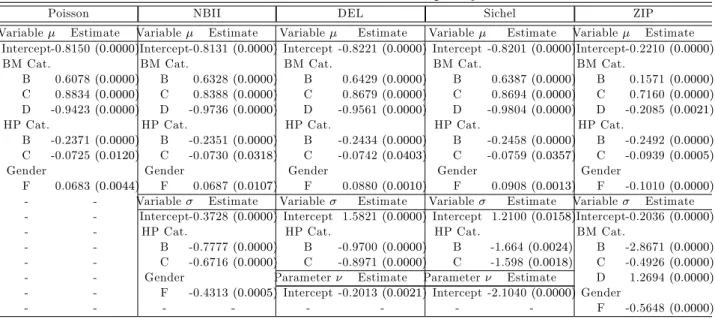
Table 1: Results of the Fitted Claim Frequency Models
Poisson NBII DEL Sichel ZIP
Variable Estimate Variable Estimate Variable Estimate Variable Estimate Variable Estimate Intercept-0.8150(0:0000)Intercept-0.8131(0:0000) Intercept -0.8221(0:0000) Intercept -0.8201(0:0000)Intercept-0.2210(0:0000)
BM Cat. BM Cat. BM Cat. BM Cat. BM Cat.
B 0.6078(0:0000) B 0.6328(0:0000) B 0.6429(0:0000) B 0.6387(0:0000) B 0.1571(0:0000)
C 0.8834(0:0000) C 0.8388(0:0000) C 0.8679(0:0000) C 0.8694(0:0000) C 0.7160(0:0000)
D -0.9423(0:0000) D -0.9736(0:0000) D -0.9561(0:0000) D -0.9804(0:0000) D -0.2085(0:0021)
HP Cat. HP Cat. HP Cat. HP Cat. HP Cat.
B -0.2371(0:0000) B -0.2351(0:0000) B -0.2434(0:0000) B -0.2458(0:0000) B -0.2492(0:0000)
C -0.0725(0:0120) C -0.0730(0:0318) C -0.0742(0:0403) C -0.0759(0:0357) C -0.0939(0:0005)
Gender Gender Gender Gender Gender
F 0.0683(0:0044) F 0.0687(0:0107) F 0.0880(0:0010) F 0.0908(0:0013) F -0.1010(0:0000)
- - Variable Estimate Variable Estimate Variable Estimate Variable Estimate - - Intercept-0.3728(0:0000) Intercept 1.5821(0:0000) Intercept 1.2100(0:0158)Intercept-0.2036(0:0000)
- - HP Cat. HP Cat. HP Cat. BM Cat.
- - B -0.7777(0:0000) B -0.9700(0:0000) B -1.664(0:0024) B -2.8671(0:0000)
- - C -0.6716(0:0000) C -0.8971(0:0000) C -1.598(0:0018) C -0.4926(0:0000)
- - Gender Parameter Estimate Parameter Estimate D 1.2694(0:0000)
- - F -0.4313(0:0005) Intercept -0.2013(0:0021) Intercept -2.1040(0:0000)Gender
- - - F -0.5648(0:0000)
From Table 1 we observe, for all frequency models, that BM category A, HP category A and male drivers are the reference categories of . HP category A and male drivers are the reference categories for in the case of the NBII model. HP category A is the reference category for in the case of the Delaporte and Sichel models. BM category A and male drivers are the reference categories for in the case of the ZIP model. Furthermore, we see that HP category appears in model equations for both and in the case of the NBII, Delaporte and Sichel models. Gender appears in model equations for both and in the case of the NBII and ZIP models. BM category appears in the models equation for both and in the case of the ZIP model. These a priori rating variables do not always have a similar e¤ect (positive and/or negative) on and
:
1 7
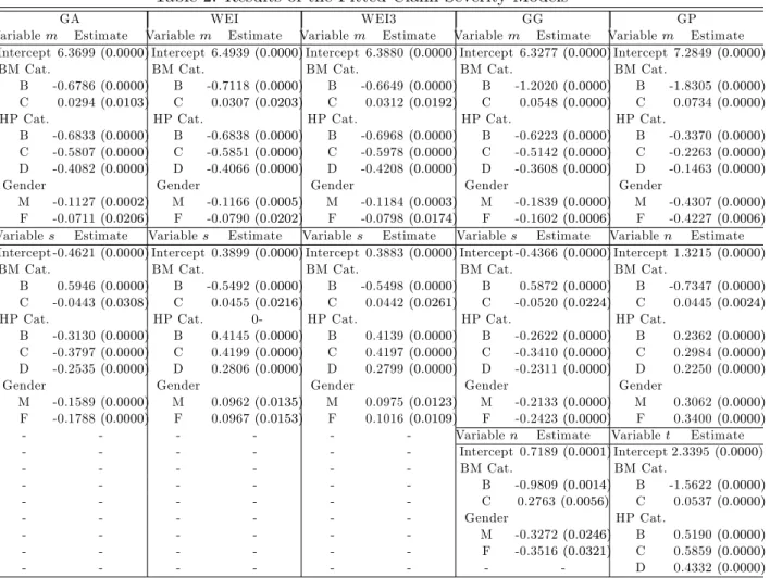
Table 2: Results of the Fitted Claim Severity Models
GA WEI WEI3 GG GP
Variablem Estimate Variablem Estimate Variablem Estimate Variablem Estimate Variablem Estimate Intercept 6.3699(0:0000)Intercept 6.4939(0:0000)Intercept 6.3880(0:0000)Intercept 6.3277(0:0000)Intercept 7.2849(0:0000)
BM Cat. BM Cat. BM Cat. BM Cat. BM Cat.
B -0.6786(0:0000) B -0.7118(0:0000) B -0.6649(0:0000) B -1.2020(0:0000) B -1.8305(0:0000)
C 0.0294(0:0103) C 0.0307(0:0203) C 0.0312(0:0192) C 0.0548(0:0000) C 0.0734(0:0000)
HP Cat. HP Cat. HP Cat. HP Cat. HP Cat.
B -0.6833(0:0000) B -0.6838(0:0000) B -0.6968(0:0000) B -0.6223(0:0000) B -0.3370(0:0000)
C -0.5807(0:0000) C -0.5851(0:0000) C -0.5978(0:0000) C -0.5142(0:0000) C -0.2263(0:0000)
D -0.4082(0:0000) D -0.4066(0:0000) D -0.4208(0:0000) D -0.3608(0:0000) D -0.1463(0:0000)
Gender Gender Gender Gender Gender
M -0.1127(0:0002) M -0.1166(0:0005) M -0.1184(0:0003) M -0.1839(0:0000) M -0.4307(0:0000)
F -0.0711(0:0206) F -0.0790(0:0202) F -0.0798(0:0174) F -0.1602(0:0006) F -0.4227(0:0006)
Variables Estimate Variables Estimate Variables Estimate Variables Estimate Variablen Estimate Intercept -0.4621(0:0000)Intercept 0.3899(0:0000)Intercept 0.3883(0:0000)Intercept -0.4366(0:0000)Intercept 1.3215(0:0000)
BM Cat. BM Cat. BM Cat. BM Cat. BM Cat.
B 0.5946(0:0000) B -0.5492(0:0000) B -0.5498(0:0000) B 0.5872(0:0000) B -0.7347(0:0000)
C -0.0443(0:0308) C 0.0455(0:0216) C 0.0442(0:0261) C -0.0520(0:0224) C 0.0445(0:0024)
HP Cat. HP Cat. 0- HP Cat. HP Cat. HP Cat.
B -0.3130(0:0000) B 0.4145(0:0000) B 0.4139(0:0000) B -0.2622(0:0000) B 0.2362(0:0000)
C -0.3797(0:0000) C 0.4199(0:0000) C 0.4197(0:0000) C -0.3410(0:0000) C 0.2984(0:0000)
D -0.2535(0:0000) D 0.2806(0:0000) D 0.2799(0:0000) D -0.2311(0:0000) D 0.2250(0:0000)
Gender Gender Gender Gender Gender
M -0.1589(0:0000) M 0.0962(0:0135) M 0.0975(0:0123) M -0.2133(0:0000) M 0.3062(0:0000)
F -0.1788(0:0000) F 0.0967(0:0153) F 0.1016(0:0109) F -0.2423(0:0000) F 0.3400(0:0000)
- - - Variablen Estimate Variablet Estimate
- - - Intercept 0.7189(0:0001)Intercept 2.3395(0:0000) - - - BM Cat. BM Cat. - - - B -0.9809(0:0014) B -1.5622(0:0000) - - - C 0.2763(0:0056) C 0.0537(0:0000) - - - Gender HP Cat. - - - M -0.3272(0:0246) B 0.5190(0:0000) - - - F -0.3516(0:0321) C 0.5859(0:0000) - - - D 0.4332(0:0000)
The results summarized in Table 2 show that BM category A, HP category A and ‡eet vehicles used by both male or female drivers are the reference categories formandsin the case of Gamma, Weibull, Weibull Type III and Generalized Gamma models. BM category A, HP category A and ‡eet vehicles are the reference categories form andn, and BM category A and HP category A are the reference categories for t in the case of the Generalized Pareto model. Note also that BM category, HP category and gender appear in the model equations for both
m and s in the case of the Gamma, Weibull and Weibull Type III and Generalized Gamma models. Furthermore, in the case of the Generalized Gamma model, BM category and gender are also in the model equations for n: Finally, in the case of the Generalized Pareto model we observe that BM category, HP category and gender appear in the model equations for both m
and n; and BM category and HP category are in the model equations fort: These explanatory variables do not always have the same e¤ect (positive and/or negative) on the parameters m,
s,nand t.
Most of the models presented in Tables 1 and 2, their reparameterizations and special cases have already been employed for modelling claim frequency/severity data. However, as we have already mentioned, the commonly used speci…cation that only the mean claim fre-quency/severity is modelled in terms of risk factors was widely accepted for ratemaking. Also, the results for the location parameter of the claim frequency/severity models are in line with the existing results, based on the examination of the relative data sets, in recent actuarial lit-erature research. Speci…cally, as expected, the values of the estimated regression coe¢ cients of the explanatory variables for this parameter will lead to mean claim frequency/severity values which will not di¤er much under di¤erent distributional assumptions. Within the framework we adopted, the systematic part of these models was expanded to allow modelling of all the
parameters of the claim frequency/severity distribution as functions of a priori rating variables. This approach is especially suited to modelling insurance response data which often exhibit het-erogeneity, i.e., a situation where the scale or shape of the distribution of the response variable changes with explanatory variables. Furthermore, joint modelling of all the parameters in an a priori ratemaking scheme breaks the nexus between the mean and variance implied by the standard procedure using GLM models, leading to a more complete comparison of these models through their variance values. Finally, in this way we will be able to use all the available in-formation in the estimation of the claim frequency/severity distribution in order to group risks with similar risk characteristics and to establish fair premium rates. Furthermore, our analysis shows that the employment of more advanced models that capture the stylized characteristics of the data is bene…cial for the insurance company.
3.2 Models Comparison
So far, we have several competing models for the claim frequency and severity components. The di¤erences between models produce di¤erent premiums. Consequently, to distinguish between these models, this section compares them so as to select the best for each case. As suggested by Rigby and Stasinopoulos (2005, 2009) the models have been calibrated with respect to Generalized Akaike Information Criterion (GAIC) which is valid for both nested or non-nested model comparisons. The Generalized Akaike Information Criterion (GAIC) is de…ned as
GAIC = ^D+ df; (32)
whereD^ = 2^lis the …tted (global) deviance,^lis the …tted log-likelihood,df is the degrees of freedom used in the model (i.e. the sum of the degrees of freedom used for the location, scale and shape parameters) and is a constant. The Akaike information criterion (AIC) and the Schwartz Bayesian criterion (SBC) are special cases of the GAIC. Speci…cally, if we let = 2
we have the AIC, while if we let = log (n) we have the SBC.
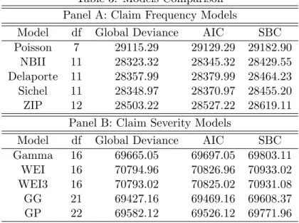
The resulting Global Deviance, AIC and SBC are given in Table 3 for the di¤erent claim frequency (Panel A) and claim severity (Panel B) …tted models.
Table 3: Models Comparison Panel A: Claim Frequency Models
Model df Global Deviance AIC SBC
Poisson 7 29115.29 29129.29 29182.90 NBII 11 28323.32 28345.32 28429.55 Delaporte 11 28357.99 28379.99 28464.23 Sichel 11 28348.97 28370.97 28455.20
ZIP 12 28503.22 28527.22 28619.11
Panel B: Claim Severity Models
Model df Global Deviance AIC SBC
Gamma 16 69665.05 69697.05 69803.11
WEI 16 70794.96 70826.96 70933.02
WEI3 16 70793.02 70825.02 70931.08
GG 21 69427.16 69469.16 69608.37
GP 22 69582.12 69526.12 69771.96
Overall, with respect to the Global Deviance, AIC and SBC indices, from Panel A we observe the best …tted claim frequency model is the Negative Binomial Type II model, followed closely by the Sichel and Delaporte models. From the claim severity models in Panel B we see that the best …tting performances are provided by the Generalized Gamma model followed
by the Generalized Pareto and Gamma models. Negative Binomial Type II and Generalized Gamma capture more e¢ ciently the stylized characteristics of the data, such as overdispersion of the number of claims and the tail behaviour of losses and performed better than the other distributions.
3.3 A Priori Risk Classi…cation
In this subsection di¤erences between the claim frequency and severity models, presented in Sections 2 and 3 respectively, are analyzed through the mean and the variance of the number and costs of claims of the policyholders who belong to di¤erent risk classes, which are determined by the availability of the relevant a priori characteristics.
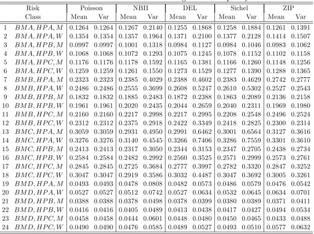
The …nal a priori ratemaking for the claim frequency models contains 24 classes. The es-timated expected annual claim frequency and the variance for each risk class are obtained by Eqs (2, 4, 8, 12 and 15) and the Eqs (2, 5, 9, 13 and 16) for the case of the Poisson, Nega-tive Binomial Type II (NBII), Delaporte (DEL), Sichel and Zero-In‡ated Poisson (ZIP) model respectively. The results are summarized in Table 4. As expected, the variance of the NBII, Delaporte, Sichel and ZIP model exceeds the mean and these models allow for overdispersion. Furthermore, we observe that the biggest di¤erences lie in the variance values of these models. For example, the variance of the expected number of claims for a man who belongs to BM category A and has a car that belongs to HP category A, i.e. for the reference class, is equal to 0.1264, 0.2140, 0.1868, 0.1884 and 0.1391 while the variance of the expected number of claims for a woman who shares common characteristics is equal to 0.1354, 0.1964, 0.2100, 0.2128 and 0.1507 in the case of the Poisson, NBII, Delaporte, Sichel and ZIP model respectively.
Table 4: A Priori Risk Classi…cation Using Claim Frequency Models
Risk Poisson NBII DEL Sichel ZIP
Class Mean Var Mean Var Mean Var Mean Var Mean Var 1 BM A; HP A; M 0.1264 0.1264 0.1267 0.2140 0.1255 0.1868 0.1258 0.1884 0.1261 0.1391 2 BM A; HP A; W 0.1354 0.1354 0.1357 0.1964 0.1371 0.2100 0.1377 0.2128 0.1414 0.1507 3 BM A; HP B; M 0.0997 0.0997 0.1001 0.1318 0.0984 0.1127 0.0984 0.1046 0.0983 0.1062 4 BM A; HP B; W 0.1068 0.1068 0.1072 0.1293 0.1075 0.1245 0.1078 0.1152 0.1102 0.1158 5 BM A; HP C; M 0.1176 0.1176 0.1178 0.1592 0.1165 0.1381 0.1166 0.1260 0.1148 0.1256 6 BM A; HP C; W 0.1259 0.1259 0.1261 0.1550 0.1273 0.1529 0.1277 0.1390 0.1288 0.1365 7 BM B; HP A; M 0.2323 0.2323 0.2385 0.4029 0.2388 0.4602 0.2383 0.4629 0.2742 0.2777 8 BM B; HP A; W 0.2486 0.2486 0.2555 0.3699 0.2608 0.5247 0.2610 0.5302 0.2527 0.2543 9 BM B; HP B; M 0.1832 0.1832 0.1885 0.2483 0.1872 0.2388 0.1863 0.2089 0.2136 0.2158 10 BM B; HP B; W 0.1961 0.1961 0.2020 0.2435 0.2044 0.2659 0.2040 0.2311 0.1969 0.1980 11 BM B; HP C; M 0.2160 0.2160 0.2217 0.2998 0.2217 0.2995 0.2208 0.2548 0.2496 0.2524 12 BM B; HP C; W 0.2312 0.2312 0.2375 0.2918 0.2422 0.3349 0.2418 0.2825 0.2300 0.2314 13 BM C; HP A; M 0.3059 0.3059 0.2931 0.4950 0.2991 0.6462 0.3001 0.6564 0.3127 0.3616 14 BM C; HP A; W 0.3276 0.3276 0.3140 0.4545 0.3266 0.7406 0.3286 0.7559 0.3301 0.3610 15 BM C; HP B; M 0.2413 0.2413 0.2317 0.3050 0.2344 0.3153 0.2347 0.2705 0.2438 0.2734 16 BM C; HP B; W 0.2584 0.2584 0.2482 0.2992 0.2560 0.3525 0.2571 0.2999 0.2573 0.2761 17 BM C; HP C; M 0.2845 0.2845 0.2725 0.3684 0.2777 0.3997 0.2782 0.3320 0.2847 0.3252 18 BM C; HP C; W 0.3047 0.3047 0.2919 0.3586 0.3032 0.4487 0.3047 0.3692 0.3005 0.3261 19 BM D; HP A; M 0.0493 0.0493 0.0478 0.0808 0.0482 0.0573 0.0486 0.0579 0.0476 0.0542 20 BM D; HP A; W 0.0527 0.0527 0.0512 0.0742 0.0527 0.0634 0.0532 0.0645 0.0634 0.0701 21 BM D; HP B; M 0.0388 0.0388 0.0378 0.0498 0.0378 0.0399 0.0380 0.0389 0.0371 0.0411 22 BM D; HP B; W 0.0416 0.0416 0.0405 0.0489 0.0413 0.0438 0.0417 0.0427 0.0494 0.0534 23 BM D; HP C; M 0.0458 0.0458 0.0444 0.0601 0.0448 0.0480 0.0450 0.0465 0.0433 0.0488 24 BM D; HP C; W 0.0490 0.0490 0.0476 0.0585 0.0489 0.0527 0.0493 0.0510 0.0577 0.0632
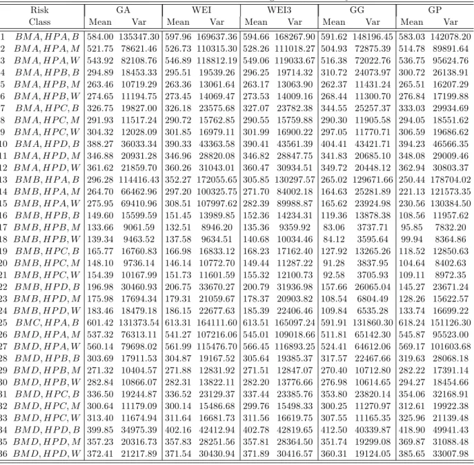
The …nal a priori ratemaking for the claim severity models contains 36 classes. Table 5 gives the estimated expected claim severity and the variance for each risk class obtained from the Gamma (GA), Weibull (WEI), Weibull Type III (WEI3), Generalized Gamma (GG) and
Generalized Pareto (GP) model according to the Eqs (18, 21, 24, 27 and 30) and the Eqs (19, 22, 25, 28 and 31) respectively. As expected, similarly to the case of the claim frequency models, we see that the biggest di¤erences between the claim severity models lie in their variance values. For instance, the variance of the expected claim costs for a ‡eet vehicle that belongs to HP category A, used by both a man and a woman, and belongs to BM category A, i.e. for the reference class, is equal to 135347.30, 169637.36, 168267.90, 148196.45 and 142078.20, while the variance of the expected claim costs for a private car that belongs to HP category A and is used by a man who belongs to BM category A is equal to 78621.46, 110315.30, 111018.27, 72875.39 and 89891.64 in the case of the Gamma, WEI, WEI3, Generalized Gamma and Generalized Pareto model.
Table 5: A Priori Risk Classi…cation Using Claim Severity Models
Risk GA WEI WEI3 GG GP
Class Mean Var Mean Var Mean Var Mean Var Mean Var
1 BM A; HP A; B 584.00 135347.30 597.96 169637.36 594.66 168267.90 591.62 148196.45 583.03 142078.20 2 BM A; HP A; M 521.75 78621.46 526.73 110315.30 528.26 111018.27 504.93 72875.39 514.78 89891.64 3 BM A; HP A; W 543.92 82108.76 546.89 118812.19 549.06 119033.67 516.38 72022.76 536.75 95624.76 4 BM A; HP B; B 294.89 18453.33 295.51 19539.26 296.25 19714.32 310.72 24073.97 300.72 26138.91 5 BM A; HP B; M 263.46 10719.29 263.36 13061.64 263.17 13063.90 262.37 11431.24 265.51 16207.29 6 BM A; HP B; W 274.65 11194.75 273.45 14069.47 273.53 14009.16 268.44 11300.70 276.84 17199.88 7 BM A; HP C; B 326.75 19827.00 326.18 23575.68 327.07 23782.38 344.55 25257.37 333.03 29934.69 8 BM A; HP C; M 291.93 11517.24 290.72 15762.85 290.55 15759.88 290.30 11905.58 294.05 18551.62 9 BM A; HP C; W 304.32 12028.09 301.85 16979.11 301.99 16900.22 297.05 11770.71 306.59 19686.62 10 BM A; HP D; B 388.27 36033.34 390.33 43363.58 390.41 43561.39 404.41 43421.71 394.23 46566.35 11 BM A; HP D; M 346.88 20931.28 346.96 28820.08 346.82 28847.75 341.83 20685.10 348.08 29009.46 12 BM A; HP D; W 361.62 21859.70 360.26 31043.01 360.47 30934.51 349.72 20448.12 362.94 30803.37 13 BM B; HP A; B 296.28 114416.43 352.27 172055.65 305.85 130297.57 265.02 129671.66 250.44 178704.02 14 BM B; HP A; M 264.70 66462.96 297.20 100325.75 271.70 84002.18 164.63 25281.89 221.13 121573.35 15 BM B; HP A; W 275.95 69410.96 308.51 107997.62 282.39 89988.87 165.62 23924.98 230.56 130384.50 16 BM B; HP B; B 149.60 15599.59 151.45 13989.85 152.36 14234.31 119.36 13878.38 108.56 11957.62 17 BM B; HP B; M 133.66 9061.59 132.51 8946.20 135.36 9359.92 83.06 3737.71 95.85 7832.20 18 BM B; HP B; W 139.34 9463.52 137.58 9634.51 140.68 10034.46 84.12 3595.64 99.94 8364.86 19 BM B; HP C; B 165.77 16760.83 166.98 16833.12 168.23 17162.40 127.92 13265.26 118.52 12850.63 20 BM B; HP C; M 148.10 9736.14 146.14 10772.70 149.44 11287.22 91.28 3837.95 104.64 8402.63 21 BM B; HP C; W 154.39 10167.99 151.73 11601.59 155.32 12100.73 92.58 3705.93 109.11 8972.35 22 BM B; HP D; B 196.98 30460.93 206.75 33670.27 200.79 31936.98 157.66 26065.04 145.27 23671.24 23 BM B; HP D; M 175.98 17694.34 179.31 21059.67 178.37 20903.82 108.54 6804.49 128.26 15622.57 24 BM B; HP D; W 183.46 18479.18 186.15 22677.63 185.39 22406.46 109.84 6535.28 133.74 16699.22 25 BM C; HP A; B 601.42 131373.54 613.31 164111.60 613.51 165097.24 591.91 131860.30 618.24 151126.30 26 BM D; HP A; M 537.32 76313.11 541.27 107216.06 545.01 109018.66 511.81 65142.30 545.87 95523.00 27 BM D; HP A; W 560.14 79698.02 561.99 115476.70 566.45 116893.25 524.41 64612.06 569.17 101603.68 28 BM D; HP B; B 303.69 17911.53 304.87 19167.52 305.64 19385.37 317.57 22467.66 319.63 28068.18 29 BM D; HP B; M 271.32 10404.57 271.88 12831.92 271.51 12847.07 270.40 10712.80 282.22 17391.14 30 BM D; HP B; W 282.84 10866.07 282.31 13822.11 282.20 13776.66 276.98 10614.65 294.27 18454.66 31 BM D; HP C; B 336.50 19244.87 336.52 23129.37 337.44 23385.76 353.80 23820.14 354.06 32168.91 32 BM D; HP C; M 300.64 11179.09 300.14 15486.68 299.76 15498.33 300.25 11270.97 312.61 19922.38 33 BM D; HP C; W 313.40 11674.94 311.64 16681.73 311.56 16619.75 307.55 11165.35 325.96 21139.48 34 BM D; HP D; B 399.85 34975.39 402.16 42412.94 402.78 42819.65 412.50 40339.87 418.90 49941.43 35 BM D; HP D; M 357.23 20316.73 357.83 28251.56 357.81 28364.50 351.74 19299.08 369.87 31088.48 36 BM D; HP D; W 372.41 21217.89 371.54 30430.94 371.89 30416.57 360.31 19124.05 385.65 33007.98
Overall, the results summarized in Tables 4 and 5 show the following trends by type of frequency/severity model as to which the lowest/highest variances are observed. Firstly, from Table 4 we see that the NBII model has the highest variance values among all models in eleven
risk classes. The Delaporte model has the highest variance values among all models in six risk classes, while it has the lowest variance value among all mixed Poisson models18 in one risk class. The Sichel model has the highest variance values among all models in …ve risk classes, while it has the lowest variance values among all mixed Poisson models in eight risk classes. The ZIP model has the highest variance values among all models in two risk classes, while it has the lowest variance values among all mixed Poisson models in …fteen risk classes. Secondly, from Table 5 we observe that the Gamma model has the highest variance value among all models in one risk class, while it has the lowest variance values among all models in fourteen risk classes. The Weibull model has the highest variance values among all models in …ve risk classes. The Weibull Type III model has the highest variance values among all models in ten risk classes. The Generalized Gamma model has the has the lowest variance values among all models in nineteen risk classes. The Generalized Pareto model has the highest variance value among all models in twenty risk classes, while it has the lowest variance values among all models in three risk classes.
The claim frequency and severity models are better compared through their variance values, leading to a better classi…cation of the policyholders and thus modelling jointly the location, scale and shape parameters in terms of a priori rating variables is justi…ed because it enables us to use all the available information in the estimation of these values through the use of the important a priori rating variables for the number and the costs of claims respectively.
3.4 Calculation of the Premiums According to the Expected Value and Standard Deviation Principles
Consider a policyholder i who belongs to a group of policyholders, whose number of claims, denoted asKi;are independent, fori= 1; ::; n. LetXi;k be the cost of thekth claim reported by
the policyholderiand assume that the individual claim costsXi;1;Xi;2; :::; Xi;nare independent.
It is assumed that the number of claims of each policyholder that belongs to a certain group is independent of the severity of each claim in order to deal with the frequency and the severity components separately.
A premium principle is a rule for assigning a premium to an insurance risk. In this section the premiums rates will be calculated via two well-known premium principles, the expected value and the standard deviation premium principles. More details about the use of the expected value premium principle in MTPL insurance can be found in Lemaire (1995). Furthermore, regarding the use of the standard deviation premium principle one can refer to Bühlmann (1970) and Lemaire (1995) who used the variance principle in MTPL insurance, which is closely related to the standard deviation principle. The standard deviation principle can be used as an alternative and complementary of the expected value principle. It provides a more complete picture to the actuary since it takes into account an additional characteristic of the distribution, i.e. the standard deviation of the number of claims and of losses.
The premium rates calculated according to the expected value principle are given by
P1 = (1 +w1)E(Ki) (1 +w2)E(Xi;k); (33)
wherew1 >0 andw2 >0 are risk loads.
The premium rates calculated according to the standard deviation principle are given by
P2 = h E(Ki) +!1 p V ar(Ki) i E(Xi;k) +!2 q V ar(Xi;k) ; (34) 1 8
The Poisson regression model has the lowest variance values among all models since they are equal to its mean values.
where!1 >0 and!2 >0 are risk loads.
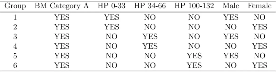
In the following example (Table 6), six di¤erent groups of policyholders have been considered. In Table 6 a ‘YES’indicates the presence of the characteristic corresponding to the column.
Table 6: The Six Di¤erent Groups of Policyholders to Be Compared Group BM Category A HP 0-33 HP 34-66 HP 100-132 Male Female
1 YES YES NO NO YES NO
2 YES YES NO NO NO YES
3 YES NO YES NO YES NO
4 YES NO YES NO NO YES
5 YES NO NO YES YES NO
6 YES NO NO YES NO YES
We will calculate the premiums P1 and P2 that must be paid by a speci…c group of
poli-cyholders based on the alternative models for assessing claim frequency and the various claim severity models. We assume that w1 =w2 =!1 =!2 = 101. The premiums P1 and P2 are
ob-tained in Table 7 by substituting into Eqs (33 and 34) the corresponding E(Ki) and V ar(Ki);
and E(Xi;k) and V ar(Xi;k) values to these six di¤erent groups of policyholders, which were
displayed in Tables 4 and 5 for the case of the Poisson, NBII, Delaporte, Sichel and ZIP, and the Gamma, Weibull, Weibull Type III, Generalized Gamma and Generalized Pareto regression models for location scale and shape respectively.
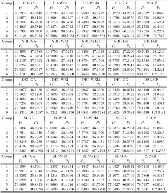
From Table 7 consider, for instance, a man who belongs to BM category A and has a car with a HP between 34-66. In the case of the Poisson model and the corresponding claim severity models, P1 is equal to 31.78, 31.77, 31.75, 31.65 and 32.03 euros, whileP2 equals 35.95, 36.07,
36.05, 35.85 and 36.5 euros. In the case of the NBII model and the corresponding claim severity models, P1 is equal to 31.91, 31.90, 31.88, 31.78 and 32.16 euros, whileP2 equals 37.35, 37.48,
37.46, 37.25 and 37.95 euros. In the case of the Delaporte model and the corresponding claim severity models,P1 is equal to 31.37, 31.36, 31.33, 31.24 and 31.61 euros, whileP2 equals 36.14,
36.26, 36.24, 36.04 and 36.72 euros. In the case of the Sichel model and the corresponding severity models,P1 is equal to 31.37, 31.36, 31.33, 31.24 and 31.61 euros, whileP2 equals 35.80,
35.93, 35.90, 35.70 and 36.38 euros. In the case of the ZIP model and the corresponding claim severity models,P1 is equal to 31.34, 31.33, 31.30, 31.20 and 31.58 euros, whileP2 equals 35.84,
35.97, 35.94, 35.74 and 36.42 euros. Overall, we observe that all the claim frequency models which were combined with the Generalized Gamma model for assessing claim severity have the lowestP1 and P2 values among their combinations with the other claim severity models. Also,
PO-GP, NBII-GP, DEL-GP, SI-GP and ZIP-GP have the highestP1 and P2 values in groups 1,
2, 3 and 4, while PO-WEI3, NBII-WEI3, DEL-WEI3, SI-WEI3 and ZIP-WEI3 have the highest
P1 and P2 values in groups 5 and 6 among their combinations with the other claim severity
models. Finally, with respect to the NBII and GG models which performed best, we see that NBII-GG has the lowestP1 values in groups 2, 4 and 6 and the lowestP2 values in groups 2 and
6 among all the combinations of the mixed Poisson models for approximating claim frequency and the claim severity models.
Table 7: Premium Rates Calculated Via the Expected Value and Standard Deviation Principles
Group PO-GA PO-WEI PO-WEI3 PO-GG PO-GP
P1 P2 P1 P2 P1 P2 P1 P2 P1 P2 1 40.2946 44.3448 40.2793 44.5028 40.2503 44.4722 40.1279 44.2231 40.6082 45.0619 2 44.9970 49.1158 44.8004 49.1297 44.8135 49.1391 43.9796 48.0550 45.3558 49.9293 3 31.7830 35.9450 31.7710 36.0730 31.7480 36.0482 31.6515 35.8463 32.0303 36.5261 4 35.4925 39.7840 35.3374 39.7953 35.3477 39.8030 34.6900 38.9248 35.7755 40.4430 5 79.7985 89.0400 80.5602 90.6845 80.7942 90.9493 77.2260 86.1468 78.7325 88.2257 6 89.1126 98.5955 89.5992 100.1082 89.9547 100.4874 84.6006 93.5402 87.9379 97.7515
Group NBII-GA NBII-WEI NBII-WEI3 NBII-GG NBII-GP
P1 P2 P1 P2 P1 P2 P1 P2 P1 P2 1 40.3903 47.3588 40.3750 47.5275 40.3458 47.4948 40.2232 47.2290 40.7045 48.1246 2 45.0967 51.3464 44.9000 51.3610 44.9128 51.3708 44.0770 50.2374 45.4563 52.1968 3 31.9105 37.3493 31.8984 37.4824 31.8754 37.4566 31.7785 37.2468 32.1588 37.9532 4 35.6254 40.8331 35.4700 40.8447 35.4801 40.8525 34.8200 39.9513 35.9095 41.5094 5 79.9880 95.0917 80.7514 96.8480 80.9860 97.1309 77.4093 92.0020 78.9194 94.2221 6 89.3100 103.0732 89.7977 104.6550 90.1540 105.0510 84.7881 97.7883 88.1327 102.1909
Group DEL-GA DEL-WEI DEL-WEI3 DEL-GG DEL-GP
P1 P2 P1 P2 P1 P2 P1 P2 P1 P2 1 40.0077 46.1980 39.9925 46.3625 39.9637 46.3306 39.8422 46.0711 40.3190 46.9449 2 45.5620 52.1760 45.3630 52.1908 45.3762 52.2008 44.5318 51.0492 45.9253 53.0402 3 31.3686 36.1354 31.3567 36.2641 31.3341 36.2392 31.2388 36.0362 31.6127 36.7197 4 35.7251 40.7265 35.5690 40.7381 35.5794 40.7459 34.9173 39.8470 36.0100 41.4011 5 79.2304 92.7607 79.9866 94.4740 80.2190 94.7500 76.6762 89.7467 78.1720 91.9124 6 90.2314 104.7387 90.7241 106.3456 91.0841 106.7484 85.6628 99.3684 89.0420 103.8421
Group SI-GA SI-WEI SI-WEI3 SI-GG SI-GP
P1 P2 P1 P2 P1 P2 P1 P2 P1 P2 1 40.1034 46.3306 40.0881 46.4957 40.0592 46.4637 39.9374 46.2034 40.4154 47.0800 2 45.7614 52.4340 45.5614 52.4489 45.5748 52.4590 44.7267 51.3016 46.1263 53.3025 3 31.3686 35.7989 31.3567 35.9264 31.3341 35.9017 31.2388 35.7006 31.6127 36.3777 4 35.8248 40.4289 35.6683 40.4404 35.6787 40.4481 35.0148 39.5558 36.1105 41.0985 5 79.4197 93.0272 80.1778 94.7453 80.4107 95.0221 76.8594 90.0045 78.3588 92.1765 6 90.6263 105.2565 91.1212 106.8714 91.4827 107.2762 86.0377 99.8600 89.4317 104.3555
Group ZIP-GA ZIP-WEI ZIP-WEI3 ZIP-GG ZIP-GP
P1 P2 P1 P2 P1 P2 P1 P2 P1 P2 1 40.1990 44.7401 40.1837 44.8994 40.1547 44.8685 40.0327 44.6172 40.5118 45.4635 2 46.9910 51.4043 46.7857 51.4189 46.7993 51.4287 45.9285 50.2941 47.3657 52.2557 3 31.3367 35.8390 31.3248 35.9666 31.3022 35.9420 31.2071 35.7406 31.5806 36.4185 4 36.6224 41.1386 36.4624 41.1503 36.4730 41.1582 35.7943 40.2502 36.9144 41.8200 5 79.6091 89.8335 80.3690 91.4926 80.6024 91.7600 77.0427 86.9146 78.5457 89.0120 6 93.0615 103.1895 93.5696 104.7726 93.9409 105.1700 88.3495 97.8986 91.8347 102.3061
4
Conclusions
In this paper, we examined the use of regression models for location, scale and shape for pricing risks through ratemaking based on a priori risk classi…cation. Speci…cally, we assumed that the number of claims was distributed according to a Poisson, Negative Binomial Type II, the Delaporte, Sichel and Zero-In‡ated Poisson and that the losses were distributed according to a Gamma, Weibull, Weibull Type III, Generalized Gamma and Generalized Pareto regression model for location, scale and shape respectively. These classi…cation models were calibrated employing a Generalized Akaike Information Criterion (GAIC) which is valid for both nested or non-nested model comparisons (as suggested by Rigby and Stasinopoulos, 2005 and 2009). The best …tted claim frequency model was the Negative Binomial Type II model, followed closely
by the Sichel and Delaporte models while regarding the claim severity models, the best …tting performances were provided by the Generalized Gamma model followed by the Generalized Pareto and Gamma models. Furthermore, the di¤erence between these models was analyzed through the mean and the variance of the annual number of claims and the severity of claims of the policyholders, who belong to di¤erent risk classes. The resulting a priori premiums rates were calculated via the expected value and standard deviation principles with independence between the claim frequency and severity components assumed.
Extensions to other frequency/severity regression models for location scale and shape can be obtained in a similar straightforward way. Moreover, these models are parametric and a possible line of further research is to explore the semiparametric approach and go through the ratemaking exercise when functional forms other than the linear are included, based on the generalized additive models for location scale and shape (GAMLSS) approach of Rigby and Stasinopoulos (2001, 2005 and 2009). Also see, for example, a recent paper by Klein et al. (2014) in which Bayesian GAMLSS models are employed for nonlife ratemaking and risk management.
References
[1] Boucher, J. P., M. Denuit and M. Guillen (2007). Risk Classi…cation for Claim Counts: A Comparative Analysis of Various Zero-In‡ated Mixed Poisson and Hurdle Models. North American Actuarial Journal, 11, 4, 110-131.
[2] Boucher, J. P., M. Denuit and M. Guillen (2008). Models of Insurance Claim Counts with Time Dependence Based on Generalisation of Poisson and Negative Binomial Distributions. Variance, 2, 1, 135-162.
[3] Boyer, M., G. Dionne and C. Vanasse (1992). Econometric Models of Accident Distribution. In Contributions to Insurance Economics, ed. G. Dionne, pp. xx–yy. Boston, Kluwer. [4] Bühlmann, H. (1970). Mathematical Models in Risk Theory. Springer-Verlag, New York. [5] Dean, C., J.F. Lawless and G.E. Willmot (1989). A mixed Poisson-inverse-Gaussian
regres-sion model. Canadian Journal of Statistics 17 (2), 171-181.
[6] Denuit, M. and S. Lang (2004). Nonlife Ratemaking with Bayesian GAM’s. Insurance, Mathematics and Economics 35: 627–47.
[7] Denuit, M., X. Marechal, S. Pitrebois and J. F. Walhin (2007). Actuarial Modelling of Claim Counts: Risk Classi…cation, Credibility and Bonus-Malus Systems. Wiley.
[8] Dionne, G. and C. Vanasse (1989). A generalization of actuarial automobile insurance rating models: the negative binomial distribution with a regression component. ASTIN Bulletin, 19, 199-212.
[9] Dionne, G. and C. Vanasse (1992). Automobile insurance ratemaking in the presence of asymmetrical information. Journal of Applied Econometrics, 7, 149-165.
[10] Evans, D. A. (1953). Experimental evidence concerning contagious distributions in ecology. Biometrika, 40: 186-211.
[11] Frangos, N. and S. Vrontos (2001). Design of optimal bonus-malus systems with a frequency and a severity component on an individual basis in automobile insurance. ASTIN Bulletin, 31, 1, 1-22.
[12] Gourieroux, C., A. Montfort and A. Trognon (1984 a). Pseudo maximum likelihood meth-ods: theory. Econometrica, 52, 681-700.
[13] Gourieroux, C., A. Montfort and A. Trognon (1984 b). Pseudo maximum likelihood meth-ods: applications to Poisson models. Econometrica, 52, 701-720.
[14] Green, P. J. and B.W. Silverman (1994). Nonparametric Regression and Generalized Linear Models. Chapman and Hall, London.
[15] Hastie, T.J. and R.J. Tibshirani (1990). Generalized Additive Models. Chapman and Hall, London.
[16] Heller, G. Z., M. D. Stasinopoulos, R. A. Rigby and P. de Jong (2007). Mean and dispersion modeling for policy claims costs. Scandinavian Actuarial Journal, 4, 281-292.
[17] Johnson, N. L., S. Kotz and N. Balakrishnan (1994). Continuous Univariate Distributions. Wiley.
[18] Klein, N., M. Denuit, S. Lang and T. Kneib (2014). Nonlife ratemaking and risk manage-ment with Bayesian generalized additive models for location, scale, and shape. Insurance: Mathematics and Economics, 55, 225-249.
[19] Klugman, S., H. Panjer and G. Willmot (2004). Loss Models: From Data to Decisions. New York, Wiley.
[20] Lambert, D. (1992). Zero-in‡ated Poisson Regression with an application to defects in Manufacturing. Technometrics, 34: 1-14.
[21] Lemaire, J. (1995). Bonus-Malus Systems in Automobile Insurance. Kluwer Academic Pub-lishers.
[22] Lopatatzidis, A. and P. J. Green (2000). Nonparametric quantile regression using the gamma distribution. submitted for publication.
[23] Nelder, J.A. and R.W.M. Wedderburn (1972). Generalized Linear Models. Journal of the Royal Statistical Society A, 135, 370-384.
[24] Renshaw, A.E. (1994). Modelling The Claims Process in the Presence of Covariates. ASTIN Bulletin, 24, 265-285.
[25] Rigby, R. A. and D. M. Stasinopoulos (2001). The GAMLSS project: a ‡exible approach to statistical modelling. In Klein, B. and L. Korsholm (eds.), New Trends in Statistical Modelling, Proceedings of the 16th International Workshop on Statistical Modelling, 249-256, Odense, Denmark.
[26] Rigby, R. A. and D. M. Stasinopoulos (2005). Generalized additive models for location, scale and shape, (with discussion). Applied Statistics, 54, 507-554.
[27] Rigby, R. A., D. M. Stasinopoulos and C. Akantziliotou (2008). A framework for model-ing overdispersed count data, includmodel-ing the Poisson-shifted generalized inverse Gaussian distribution. Computational Statistics and Data Analysis, 53, 381–393.
[28] Rigby, R. A. and D. M. Stasinopoulos (2009). A ‡exible regression approach using GAMLSS in R.
[29] Tzougas, G. and N. Frangos (2014). The Design of an Optimal Bonus-Malus System Based on the Sichel Distribution. Modern Problems in Insurance Mathematics. Springer Verlag.
[30] Yip, K. and K. Yau (2005). On modeling Claim Frequency Data in General Insurance with Extra Zeros. Insurance, Mathematics and Economics 36: 153-63.