Should I Stay or Should I Go?
Bayesian Inference in the
Threshold Time Varying
Parameter (TTVP) Model
Florian Huber, Gregor Kastner, Martin
Feldkircher
Research Report Series Institute for Statistics and Mathematics
Should I stay or should I go?
Bayesian inference in the threshold time varying
parameter (TTVP) model
Florian Huber∗1, Gregor Kastner1, and Martin Feldkircher2
1WU Vienna University of Economics and Business 2Oesterreichische Nationalbank (OeNB)
September 18, 2016
Abstract
We provide a flexible means of estimating time-varying parameter models in a Bayesian framework. By specifying the state innovations to be characterized trough a threshold process that is driven by the absolute size of parameter changes, our model detects at each point in time whether a given regression coefficient is con-stant or time-varying. Moreover, our framework accounts for model uncertainty in a data-based fashion through Bayesian shrinkage priors on the initial values of the states. In a simulation, we show that our model reliably identifies regime shifts in cases where the data generating processes display high, moderate, and low num-bers of movements in the regression parameters. Finally, we illustrate the merits of our approach by means of two applications. In the first application we forecast the US equity premium and in the second application we investigate the macroeco-nomic effects of a US monetary policy shock.
Keywords: Change point model, Threshold mixture innovations, Structural breaks, Shrink-age, Bayesian statistics, Monetary policy
JEL Codes: C11, C32, C52, E42.
∗Corresponding author: Florian Huber, WU Vienna University of Economics and Business, phone:
+43-1-313 2036-4534, e-mail: [email protected]. The opinions expressed in this paper are those of the authors and do not necessarily reflect the official viewpoint of the Oesterreichische Nationalbank or the Eurosystem.
1 Introduction
In the last few years, economists in policy institutions and central banks were criticized for their failure to foresee the recent financial crisis that engulfed the world economy and led to a sharp drop in economic activity. Critics argued that economists failed to predict the crisis because models commonly utilized at policy institutions back then were too simplistic. For instance, the majority of forecasting models adopted were (and possibly still are) linear and low dimensional. The former implies that the underlying structural mechanisms and the volatility of economic shocks are assumed to remain constant over time – a rather restrictive assumption. The latter implies that only little information is exploited which may be detrimental for obtaining reliable predictions.
In light of this criticism, practitioners started to develop more complex models that are capable of capturing salient features of time series commonly observed in macroe-conomics and finance. Recent research (Stock and Watson,1996;Cogley and Sargent,
2002;2005;Primiceri, 2005;Sims and Zha,2006) suggests that, at least for US data, there is considerable evidence that the influence of certain variables appears to be time-varying. This raises additional issues related to model specification and estimation. For instance, do all regression parameters vary over time? Or is time variation just limited to a specific subset of the parameter space? Moreover, as is the case with virtually any modeling problem, the question whether a given variable should be included in the model in the first place naturally arises. Apart from deciding whether parameters are changing over time, the nature of the process that drives the dynamics of the coeffi-cients also proves to be an important modeling decision.
In a recent contribution, Fr¨uhwirth-Schnatter and Wagner (2010) focus on model specification issues within the general framework of state space models. Exploiting a non-centered parametrization of the model allows them to rewrite the model in terms of a constant parameter specification, effectively capturing the steady state along with deviations from this steady state. The non-centered parameterization is subsequently used to search for appropriate model specifications, imposing shrinkage on the steady state part and the deviations from this steady state. Recent research aims to discrim-inate between inclusion/exclusion of elements of different variables and whether the associated regression coefficient is constant or time-varying (Belmonte, Koop, and Ko-robilis, 2014; Eisenstat, Chan, and Strachan, 2016; Koop and Korobilis, 2012; 2013;
Kalli and Griffin, 2014). Another strand of the literature asks whether coefficients are constant or time-varying by assuming that the innovation variance in the state equation is not constant, but is characterized by a change point process that assumes that de-pending on some exogenous stochastic process, either equals zero or is left unrestricted
(McCulloch and Tsay, 1993; Gerlach, Carter, and Kohn, 2000; Koop, Leon-Gonzalez, and Strachan,2009;Giordani and Kohn,2012).
In the present paper we adopt ideas from the literature (Nakajima and West,2013a;b;
Zhou, Nakajima, and West,2014;Kimura and Nakajima, 2016) and introduce a set of latent thresholds that control the degree of time-variation for each parameter and point in time separately. This is achieved by estimating a set of variable-specific thresholds that allows for movements in the autoregressive parameters if the proposed change of the parameter is large enough. We show that this can be achieved by assuming that the innovations of the state equation follow a threshold model that discriminates between a situation where the innovation variance is large and a case with an innovation vari-ance set equal to zero. The proposed model nests a wide variety of competing models, most notably the standard time-varying parameter model, a change-point model with an unknown number of regimes, mixtures between different models and finally the sim-ple constant parameter model. To assess systematically and a in a data-driven fashion which predictors should be included in the model, we impose a set of Normal-Gamma priors (Griffin and Brown,2010) in the spirit of Bitto and Fr¨uhwirth-Schnatter(2015) on the initial state of the system.
By means of a comprehensive simulation exercise, we asses how well the proposed model can recapture the data generating parameter paths. It turns out that the TTVP model outperforms the standard TVP model in various scenarios and for numerous data generating processes.
Moreover, we illustrate the empirical merits of our approach by two applications. In the first, we use our model to forecast the excess return of the S&P 500 stock market index. The findings indicate that, when compared to a standard TVP model with shrink-age priors on the initial state, the TTVP model provides pronounced accuracy premiums in terms of log predictive scores. When point forecasts are taken under consideration the results are somewhat mixed, with the TTVP outperforming during recessionary pe-riods while being slightly inferior when the full sample is taken under consideration. Both time-varying parameter models, however, markedly outperform a simple linear regression model estimated with uninformative priors.
In the second application we assess how well our approach performs in a multivari-ate context. More specifically, we extend the model to the vector autoregressive (VAR) case and apply it to investigate the effects of a contractionary US monetary policy shock over time. With respect to the size of estimated effects and the behavior of the vari-ables under consideration, our model yields results that are in line with the literature. In addition, we find evidence for considerable changes in the effect of the monetary policy shock over time. More specifically, our results show that shocks to the federal funds rate exert most pronounced effects in the early part of our sample, while they
started to diminish from the mid-1970s onwards. The subsequent period of the Great Moderation is characterized by modest effects and little variation over time. Finally, effects tick up considerably with the outbreak of the global financial crisis.
The paper is structured as follows. Section 2 introduces the univariate model, the prior setup and the corresponding MCMC algorithm for posterior simulation. Section3
illustrates the behavior of the model by showcasing scenarios with few, moderately many, and many jumps in the state equation. Section 4 puts forth an extensive sim-ulation study to investigate how well the time-varying regression coefficients can be recovered through posterior inference. Section 5 puts forward a model extension to cater for stochastic volatility and analyses the performance of the model when applied to predict S&P 500 excess returns. Section6discusses how the model can be extended to higher dimensions within the framework of VARs and presents an application of the TTVP-VAR with stochastic volatility to a seven-dimensional macroeconomic data set. Finally, Section7concludes.
2 Econometric framework
We begin by specifying a flexible model that is capable of discriminating between con-stant and time-varying parameters at each point in time.
2.1 A threshold mixture innovation model
Consider the following dynamic regression model,
yt=x0tβt+ut, ut∼ N(0, σ2), (2.1)
where xt is a K-dimensional vector of explanatory variables and βt = (β1t, . . . , βKt)0
a vector of regression coefficients. The error term ut is assumed to be normally
dis-tributed white noise with constant variance.1 This model assumes that the relationship
between elements ofxtandytis not necessarily constant over time, but changes subject
to some law of motion forβt. Typically, researchers assume that thejth element ofβt
follows a random walk process,
βjt =βj,t−1+ejt, ejt ∼ N(0, ϑj), (2.2)
with ϑj denoting the innovation variance of the latent states. Equation (2.2) implies
that parameters evolve gradually over time, ruling out abrupt changes. While being 1For simplicity, we assume thatσ2does not change over time. However, in the empirical application
conceptually flexible, in the presence of only a few breaks in the parameters, this model generates spurious movements in the coefficients that could be detrimental for the empirical performance of the model (D’Agostino, Gambetti, and Giannone,2013).
Thus, we depart from Eq. (2.2) by specifying the innovations of the state equation
ejt to be a mixture distribution. More concretely, we specify
ejt =sjt
√
ϑjηjt, ηjt ∼ N(0,1). (2.3)
In the present framework, as opposed to the literature on mixture innovation mod-els (McCulloch and Tsay,1993; Gerlach, Carter, and Kohn, 2000; Giordani and Kohn,
2012),sjt denotes the indicator function with
sjt = 1 if |∆βjt|> dj, 0 if |∆βjt| ≤dj, (2.4)
where dj is a coefficient-specific threshold to be estimated. Equations (2.3) and (2.4)
state that if the absolute period-on-period change of βjt exceeds a threshold dj, we
assume that the change inβjt is normally distributed with zero mean and varianceϑj.
On the contrary, if the change in the parameter is too small, the innovation variance equals zero, implying thatβjt =βj,t−1, i.e., no change from period(t−1)tot.
This modeling approach provides a great deal of flexibility, nesting a plethora of sim-pler model specifications. The interesting cases are characterized by situations where
sjt equals unity only for somet. For instance, it could be the case that parameters tend
to exhibit strong movements at given points in time but stay constant for the majority of time. An unrestricted time-varying parameter model would imply that the parameters are gradually changing over time, depending on the innovation variance in Eq. (2.2). Another prominent case would be a structural break model with an unknown number of breaks (for a recent Bayesian exposition, seeKoop and Potter,2007).
The mixture innovation component in Eq. (2.3) implies that we discriminate be-tween two regimes. The first regime assumes that changes in the autoregressive pa-rameters tend to be large and important to predict yt whereas in the second regime,
these changes can be safely regarded as being zero, thus effectively leading to a con-stant parameter model over a given period of time. Compared to a standard mixture innovation model that postulatessjt as a sequence of independent Bernoulli variables,
our approach assumes that regime shifts are governed by a deterministic law of mo-tion. The main advantage of our approach relative to mixture innovation models is that instead of having to estimate a full sequence of sjt for allj, the threshold mixture
innovation model only relies on a single additional parameter per coefficient, rendering estimation of high dimensional models such as vector autoregressions (VARs) feasible. Our model is also closely related to the latent thresholding approach put forward inNakajima and West (2013a). While in their model latent thresholding discriminates between the inclusion or exclusion of a given covariate at time t, our model detects whether the associated regression coefficient can be viewed as being constant or time-varying.
The question whether a given regressor is included or excluded in our model can ef-fectively be tackled by using a variant of the non-centered parameterization (Fr¨ uhwirth-Schnatter and Wagner,2010) ofEq. (2.1):
yt=x0tβ0+x0tβˆt+ut. (2.5) The deviation from the initial state is given by βˆt = βt−β0. Equation (2.5) states that the model can be written in terms of a time-invariant part given by x0tβ0 and a time-varying componentx0tβˆt. FromEq. (2.5)it is easily seen that a given variablej is excluded from the model ifβ0j andβˆjt equals zero for allt.
2.2 Prior specification
Since our approach to estimation and inference is Bayesian, we have to specify suitable prior distributions for all parameters of the model given by Eqs. (2.1) and (2.2).
We impose a Normal-Gamma prior (Griffin and Brown, 2010) on each element of
β0, the initial state of the system,
β0j|τj ∼ N(0,2/λ2τj2), τ
2
j ∼ G(aj, aj) forj = 1, . . . , K. (2.6)
Hereby, λ2 and a
j are hyperparameters and τj2 denotes an idiosyncratic scaling
pa-rameter that applies an individual degree of shrinkage on each element of β0. The hyperparameterλ2 serves as a global shrinkage parameter that shrinks all elements of
β0 towards zero while the local shrinkage parametersτj provide enough flexibility to
also allow for non-zero values ofβ0j in the presence of a tight global prior specification.
For the global scaling parameterλ2we impose a Gamma prior,λ2 ∼ G(b0, b1),withb0
andb1 being a set of hyperparameters chosen by the researcher. In typical applications
we specifyb0andb1to render this prior effectively non-influential. For the inverse of the
innovation variance of the observation equation inEq. (2.5), we impose a Gamma prior onσ−2with hyperparametersc
distributed prior2 on the inverse of the innovation variances in the state specification in Eq. (2.2), i.e., ϑ−j1 ∼ G(r0j, r1j) for j = 1, . . . , K. Again, r0j and r1j denote scalar
hyperparameters. This choice implies that we artificially bound ϑj away from zero,
implying that in the upper regime we do not exert strong shrinkage. This is in contrast to a standard time-varying parameter model, where this prior is usually set rather tight to control the degree of time variation in the parameters (see, e.g., Primiceri, 2005). Note that in our model the degree of time variation is governed by thresholding instead. Finally, the prior specification of the baseline model is completed by imposing a uniform distributed prior on the thresholds,
dj ∼ U(π0j, π1j). (2.7)
Here,π0j andπ1j denote the boundaries of the prior that have to be specified carefully.
In our examples, we use π0j = 0.1×max|∆βTj| and π1j = max|∆βTj|, with |∆β T j| =
|(∆βj1, . . . ,∆βjT)0| being the absolute values of the full history of the latent states.
This prior bounds the thresholds away from zero, implying that a certain amount of shrinkage is always imposed on the autoregressive coefficients. Since the data is not really informative on the specific level of the threshold, using a prior that is agnostic on the specific value of the threshold (i.e., by settingπ0j = 0for allj) yields situations
where the posterior of the thresholds is strongly concentrated around zero, favoring an unrestricted TVP model. It is worth noting that even under the assumption that
π0j > 0, our framework performs well in simulations where the data is obtained from
a non-thresholded version of our model, cf., Section4. Moreover, in a situation where parameters are expected to evolve smoothly over time, the maximum period-on-period change of βjt is small, implying that 0.1×max|∆βTj| is close to zero and the model effectively shrinks movements that can safely regarded as being small.
2.3 Posterior simulation
We sample from the joint posterior distribution of the model parameters by utilizing a relatively simple Markov chain Monte Carlo (MCMC) algorithm. Conditional on the thresholdsdj, the remaining parameters can be simulated in a straightforward fashion.
After initializing the parameters using suitable starting values we iterate between the following five steps.
2Of course, it would also be possible to use a (restricted) Gamma prior onϑ
jin the spirit ofFr¨
uhwirth-Schnatter and Wagner (2010). However, we have encountered some issues with such a prior if the number of observations in the regime associated with sjt = 1is small. This stems from the fact that
the corresponding conditional posterior distribution is generalized inverse Gaussian, a distribution that is heavy tailed and under certain conditions leads to excessively large draws ofϑj.
1. We start by simulating the full history of βt, denoted as βT = (β0, . . . ,βT)0 by means of a standard forward filtering backward sampling algorithm (Carter and Kohn,1994;Fr¨uhwirth-Schnatter,1994) while conditioning on the remaining pa-rameters of the model given by Eqs. (2.1) and (2.2).
2. The inverse of the innovation variances of Eq. (2.2),ϑ−j1, j = 1, . . . , K are simu-lated from the following Gamma distributed conditional posterior distribution,
ϑ−j1|• ∼ G c0 2 + T1j 2 , c1 2 + PT t=1sjt(βjt−βjt−1)2 2 ! , (2.8) withT1j = PT
t=0sjt denoting the number of time periods that feature time
varia-tion in thejth parameter.
3. Combining the Gamma prior onτj2 with the Gaussian likelihood yields a General-ized Inverted Gaussian (GIG) distribution
τj2|• ∼ GIG aj− 1 2, β 2 j0, ajλ2 , (2.9)
where the density of the GIG(κ, χ, ψ)distribution is proportional to
zκ−1exp −1 2 χ z +ψz . (2.10)
To sample from this distribution, we use the R package GIGrvg (Leydold and H¨ormann,2015) implementing the efficient rejection sampler proposed byH¨ormann and Leydold(2013).
4. The global shrinkage parameter λ2 is sampled from a Gamma distribution given
by λ2|• ∼ G b0+ajK, b1+ aj 2 K X j=1 τj2 ! . (2.11)
5. We update the thresholds by applying K Griddy Gibbs steps (Ritter and Tanner,
1992). Due to the structure of the model, the likelihood function is independent from the data, implying that
p βTj|dj, ϑj= T Y t=1 1 p 2πsjtϑj exp −(βjt −βjt−1) 2 2sjtϑj . (2.12)
The likelihood can be straightforwardly combined with the prior in Eq. (2.7) to evaluate the conditional posterior of dj at a given candidate point.3 This
proce-dure is repeated over a fine grid of values that is determined by the prior and an approximation to the inverse cumulative distribution function of the poste-rior is constructed. This approximation is then used to perform inverse transform sampling.
6. Finally, the posterior of the inverse of the error variances of the observation equa-tion takes a standard form, namely a Gamma distribuequa-tion with
σ−2|• ∼ G c0 2 + T 2, c1 2 + PT t=1(yt−x 0 tβt)2 2 ! . (2.13)
After obtaining an appropriate number of draws, we discard the firstN as burn-in and base our inference on the remaining draws from the joint posterior.
3 Three illustrative examples
In this section we illustrate our approach by means of a rather stylized example that emphasizes how well the mixture innovation component for the state innovations per-forms when used to approximate different data generating processes (DGPs).
For demonstration purposes it proves to be convenient to start with the following simple DGP withK = 1:
yt=x01tβ1t+ut, ut∼ N(0,0.012),
β1t=β1t−1+e1t, e1t ∼ N(0, s1t×0.152).
Furthermore, we assume that the model moves through a relatively low number of possible regimes, s1t = 1 if |∆β1t|> dtrue, 0 if |∆β1t| ≤dtrue.
Finally, independently for allt, we generatex1t ∼ U(−1,1)and setβ1,0 = 0. This DGP
assumes that parameter movements have to exceed dtrue, which is set equal to 2, 2.5,
and 3 times the standard deviation of β1t. This should provide some simple intuition
on how our modeling approach performs in situation where the DGP is characterized by many, moderate and few breaks.
3Note that we avoid numerical issues related to the situations
jt = 0by using a offsetting constant
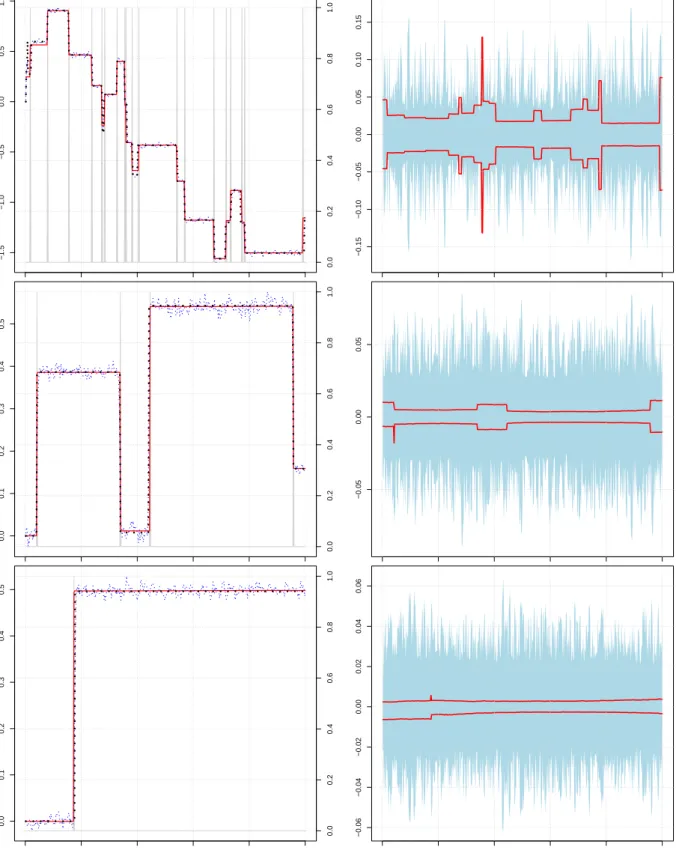
Fig. 1 shows three possible realizations ofβ1t and the corresponding estimates
ob-tained from a standard TVP model and our TTVP model. To ease comparison between the models we impose a similar prior setup for both models. Specifically, for σ−2 we
set c0 = 0.01 and c1 = 0.01, implying a rather vague prior. For the shrinkage part on β1,0 we set λ2 ∼ G(0.01,0.01) and a1 = 0.1, effectively applying heavy shrinkage on
the initial state of the system. The prior on ϑ1 is specified as in Nakajima and West
(2013a), i.e.,ϑ−11 ∼ G(3,0.03). To complete the prior setup for the TTVP model we set
π1,0 = 0.1×max|∆βT1|and π1,1 = max|∆βT1|. Finally, it is noteworthy that we specify
an off-setting constantκ0,1 = 10−7×ϑ1 that is close to zero.
The left panel ofFig. 1displays the evolution of the posterior median of a standard TVP model (in dotted blue) and of the TTVP model (in solid red) along with the actual evolution of the state vector (in dotted black). In addition, the areas shaded in gray de-pict the probability that a given coefficient moves over a certain time frame (henceforth labeled as posterior moving probability, PMP). The right panel shows the (de-meaned) posterior distribution (5th and 95th credible intervals) of the TVP model (blue shaded area) and the TTVP model (solid red lines).
At least two interesting findings emerge. First, note that in all three cases, our ap-proach detects parameter movements rather well, with PMP reaching unity in virtually all time points that feature a structural break of the corresponding parameter. By con-trast, the TVP model also tracks the actual movement of the states well but with much more high frequency variation. This is a direct consequence of the inverted Gamma prior on the state innovation variances that bound ϑ1 artificially away from zero,
irre-spective of the information contained in the likelihood (see Fr¨uhwirth-Schnatter and Wagner,2010, for a general discussion of this issue).
Second, looking at the uncertainty surrounding the median estimate (right panel of Fig. 1) reveals that our approach succeeds in shrinking the posterior uncertainty surrounding our median estimates. This is due to the fact that in periods where the true value of βt is constant, our model successfully assumes that the estimate of the coefficient at timet is also constant, whereas the TVP model imposes a certain amount of time variation. This generates additional uncertainty that inflates the posterior vari-ance, possibly leading to imprecise inference.
Thus, the TTVP model reliably detects change points in the parameters in situations where the actual number of breaks is small, moderate and large. In situations where the DGP suggests that the actual threshold equals zero, our approach still captures most of medium to low frequency noise but shrinks small movements that might, in any case, be less relevant for doing inference. If the parameters do not move at all, strong prior information is necessary to recover this from data. This is because the
0.0 0.2 0.4 0.6 0.8 1.0 0 100 200 300 400 500 −1.5 −1.0 −0.5 0.0 0.5 1.0
(a) Posterior median and true value of β1
0 100 200 300 400 500 −0.15 −0.10 −0.05 0.00 0.05 0.10 0.15
(b) Demeaned posterior distribution of β1
0.0 0.2 0.4 0.6 0.8 1.0 0 100 200 300 400 500 0.0 0.1 0.2 0.3 0.4 0.5
(a) Posterior median and true value of β1
0 100 200 300 400 500
−0.05
0.00
0.05
(b) Demeaned posterior distribution of β1
0.0 0.2 0.4 0.6 0.8 1.0 0 100 200 300 400 500 0.0 0.1 0.2 0.3 0.4 0.5
(a) Posterior median and true value of β1
0 100 200 300 400 500 −0.06 −0.04 −0.02 0.00 0.02 0.04 0.06
(b) Demeaned posterior distribution of β1
Fig. 1: Left: Evolution of the actual state vector (dotted black) along with the
poste-rior medians of the TVP model (dashed blue) and the TTVP model (solid red). Right: Demeaned posterior distribution of the TVP model (90% credible intervals in shaded blue) and the TTVP model (90% credible intervals in red).
likelihood does not carry information about thresholds when no structural breaks are present, consequently rendering weakly informative priors useless.
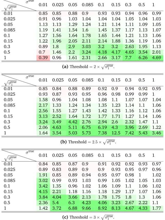
4 Simulation based evidence
In this section we illustrate the merits of our approach by performing extensive univari-ate simulation experiments under the three DGP scenarios from Section 3, i.e., many (dtrue = 2√ϑ1), moderately many (dtrue = 2.5
√
ϑ1), and few (dtrue = 3 √
ϑ1) breaks in
the state equation. We consider a square grid of different values for the innovation standard deviation in the state equation √ϑ1 and the innovation standard deviation
in the observation equation σ ranging from 0.01 to 1 for both parameters. For each possible case, a “true” path of regression coefficients {βttrue} is simulated; then, a set of exogenous predictors{xt}is drawn independently fromU(−1,1); finally, a response path{yt}is generated according toEq. (2.1).
Using the data {xt, yt} only, we then fit a TTVP as well as a TVP model, where
prior hyperparameters4 are chosen as in Section 3 and posterior inference for each
experiment is based on 7500 draws of which 2500 are discarded as burn-in. We cal-culate mean absolute deviations (MeanADs) of posterior means βˆt from the respective
data generating paths βttrue, averaged over T = 500 points in time, i.e., MeanAD =
T−1PT
t=1|βˆt−βttrue|. Each experiment is repeated 100 times and median values
rela-tive to those obtained from a standard TVP model without thresholding are reported in Table 1. We note that using root mean squared errors instead of MeanADs gives a similar overall picture. However, the benefits of thresholding are somewhat less pro-nounced, in particular for small values of σtrue (i.e., very high “signal-to-noise” ratio). The converse is true when median absolute deviations are considered, favoring TTVP in practically all scenarios unlessp
ϑtrue1 is very small. This hints at occasional outliers that are more persistent under TTVP than under TVP.
Results for DGPs with many jumps in Table 1(a)show that the TTVP performs bet-ter on a very wide range of data generating paramebet-ter values, the only exception being a very small signal (pϑtrue1 ≈ 0.01) or an extremely high signal to noise ratio (pϑtrue1 /σtrue & 30). A similar picture appears in Table 1(b) when considering mod-erately many jumps; there, TTVP outperforms TVP unless the signal is smaller than approximately 0.03. This pattern continues; in the setting with many jumps (see Ta-ble1(c)) TTVP wins for moderate and large signals (p
ϑtrue1 &0.08).
4We remark that in light of the rather large range of DGP parameters considered below, this is a very
pragmatic (and possibly not ideal) choice. Alternatively to fixing the hyperparameters independently of the DGP parameter values, one could also choose the hyperparameters dependently on the DGP param-eter values in the spirit of Empirical Bayes methods.
p ϑtrue1 σtrue 0.01 0.025 0.05 0.085 0.1 0.15 0.3 0.5 1 0.01 0.85 0.85 0.88 0.9 0.93 0.93 0.94 0.96 0.99 0.025 0.91 0.96 1.03 1.04 1.04 1.04 1.05 1.04 1.03 0.05 1.13 1.13 1.29 1.24 1.21 1.14 1.11 1.09 1.05 0.085 1.19 1.41 1.54 1.6 1.45 1.37 1.17 1.13 1.07 0.1 1.27 1.56 1.64 1.78 1.65 1.44 1.21 1.13 1.06 0.15 1.22 1.96 2.05 2.11 2.14 1.88 1.36 1.19 1.06 0.3 0.89 1.8 2.9 3.03 3.2 3.2 2.63 1.95 1.13 0.5 0.7 1.46 2.2 3.24 4.18 4.17 4.65 3.54 2.01 1 0.39 0.96 1.61 2.31 2.66 3.17 7.7 6.26 4.69
(a)Threshold= 2×pϑtrue1 .
p ϑtrue1 σtrue 0.01 0.025 0.05 0.085 0.1 0.15 0.3 0.5 1 0.01 0.85 0.84 0.88 0.89 0.92 0.9 0.94 0.92 0.95 0.025 0.93 0.87 0.93 0.95 0.96 0.98 0.99 0.99 1 0.05 1.58 0.96 1.04 1.08 1.08 1.1 1.07 1.07 1.04 0.085 2.17 1.33 1.24 1.34 1.35 1.23 1.14 1.1 1.06 0.1 2.56 1.55 1.27 1.43 1.42 1.33 1.16 1.12 1.06 0.15 3.13 2.52 1.64 1.72 1.77 1.71 1.27 1.14 1.06 0.3 3.24 3.49 4.42 2.76 2.94 2.6 2.32 1.47 1.1 0.5 2.06 4.63 5.11 6.75 6.19 4.3 3.96 2.69 1.22 1 1.64 3.54 5.03 5.73 7.38 12.5 7.42 5.43 3.46 (b)Threshold= 2.5×p ϑtrue1 . p ϑtrue1 σtrue 0.01 0.025 0.05 0.085 0.1 0.15 0.3 0.5 1 0.01 0.84 0.85 0.87 0.9 0.91 0.92 0.92 0.93 0.97 0.025 0.89 0.83 0.89 0.9 0.9 0.93 0.95 0.97 0.96 0.05 1.91 0.85 0.89 0.94 0.95 0.97 0.98 1 1.02 0.085 3.02 0.99 0.93 1.03 0.99 1.05 1.02 1.05 1.03 0.1 3.42 1.35 0.96 1.02 1.06 1.09 1.1 1.06 1.02 0.15 4.15 2.21 1.18 1.16 1.18 1.29 1.17 1.07 1.06 0.3 3.84 4.04 3.66 2.13 1.78 1.75 1.8 1.3 1.06 0.5 2.36 5.4 6.3 4.23 4.06 3.23 2.67 2.22 1.1 1 1.42 3.72 6.88 9.66 8.92 8.13 4.67 4.33 1.77 (c)Threshold= 3×p ϑtrue1 .
Table 1: Medians of relative mean absolute deviations (100 repetitions). Numbers
greater than one mean that TTVP performs better than TVP. Shading: 0.25 0.31 0.4 0.57 1 1.75 2.5 3.25 4
Without presenting the results in detail, we briefly discuss the two extreme cases: continuously varying and completely constant parameters. First, we consider the for-mer, a standard TVP DGP (dtrue = 0). It appears that the TTVP model – even though misspecified – does well against the TVP model, unless there is a very strong signal (p
ϑtrue1 large) with only tiny amounts of noise (σtrue small). Second, we investigate the simple standard regression setting with constant coefficients, i.e.,dtrue =∞ or equiva-lentlyβ1t≡β1,0 for allt= 1, ..., T = 500. Here, TTVP performs slightly worse than TVP,
in particular for low amounts of noise (σtrue small).
5 Empirical Application I: Forecasting equity price excess returns
In the first application we focus attention on predicting S&P 500 excess returns us-ing the TTVP model, a standard TVP model and a constant parameter specification. Predicting equity prices has been one of the main challenges for financial economists during the last decades. A plethora of studies emerged that draw a relationship be-tween different macroeconomic and financial fundamentals and the predictability of excess returns (Lettau and Ludvigson,2001;Ang and Bekaert,2007;Welch and Goyal,
2008; Dangl and Halling, 2012). The purpose of this application is to assess whether using the TTVP specification pays off in terms of predictive performance in a relatively high dimensional setting.
5.1 Model specification an data
The model put forward inEq. (2.1)is assumed to feature homoscedastic shocks. In this section we relax this assumption by assuming that the shocks, denoted by ht = ln(σt2),
follow an AR(1) process,
ht =µ+ρ(ht−1−µ) +νt, (5.1)
withµbeing the mean of the log-volatility andρdenoting the autoregressive coefficient. Finally,νtis a white noise error with variance given by ζ.
The prior setup adopted is the same as before except that we also have to impose priors on µ, ρ and ζ. We follow Kastner and Fr¨uhwirth-Schnatter (2014) and impose a normally distributed prior on µwith mean zero and variance 100, a Beta prior on ρ
with(ρ+ 1)/2∼ B(25,5), and a Gamma distributed prior onζ ∼ G(1/2,1/2).
The MCMC algorithm closely mirrors the one presented in Section 2 except that we sample the coefficients of the log-volatility equation and the corresponding full-history of log-volatilities by means of the algorithm outlined inKastner and Fr¨ uhwirth-Schnatter (2014), implemented in the R package stochvol (Kastner, 2016). For our
15 000 being discarded as burn-in. Looking at traditional convergence criteria indicate convergence of the Markov chain.
We use the dataset provided byWelch and Goyal(2008) and assume that the excess return is a function of a set of fundamental factors. More specifically, our benchmark regression comprises of 14 fundamental factors that the recent literature identified as having predictive power for excess returns. The dependent variable is the S&P 500 index return measured from 1926 to 2010 minus the risk free rate constructed as de-scribed in Welch and Goyal (2008). We include the following (lagged) covariates in our models. The dividend price ratio (defined as the difference between log dividends and the log of prices), the dividend yield (defined as the difference between log div-idends and the log of lagged prices), the earnings price ratio, the dividend payout ratio, the stock variance (defined as the sum of squared S&P 500 daily returns), the cross-sectional premium (see Polk, Thompson, and Vuolteenaho,2006) and the book-to-market ratio (computed as the ratio of the book value to market value for the Dow Jones Industrial Average). Furthermore, we measure corporate issuing activity by in-cluding the ratio of 12-month moving sums of net issues by stocks listed at the New York Stock Exchange (NYSE) divided by the total end-of-year market capitalization of NYSE stocks. In addition, we also include the fraction of equity issuing activity of total issu-ing activity. The next set of covariates are related to fixed income markets. We include data on treasury bills, long term yields and the term spread (measured as the difference between three-month yields on treasury bills and ten-year government bonds). To mea-sure movements in corporate bond markets we include the spread between BAA and AAA-rated corporate bond yields and the difference between long-term corporate bond and government bond returns. Finally, we include two macroeconomic quantities in the regression, namely (lagged) consumer price inflation and the investment to capital ratio (defined as the ratio of aggregate investment to aggregate capital).
5.2 Forecasting the US equity premium
We utilize a recursive forecasting design and specify the period ranging from 1926 December to 1956 December as an initial estimation period. We then consequently expand the initial estimation sample by one month until the end of the sample (2010 December) is reached. This yields a sequence of 647 monthly one-step-ahead predictive densities for the S&P 500 excess return where we rely on the root mean square error (RMSE) and the log predictive score (seeGeweke and Amisano,2010, for a discussion) to evaluate the predictive capabilities of the model.
Table 2displays the results of the forecasting exercise. Looking at the left part of the table reveals that both models that allow for drifting parameters heavily outperform a
simple linear regression framework. The strong outperformance can be attributed to the fact that the both, the TTVP and the TVP, feature stochastic volatility in the errors, a feature that typically improves density predictions markedly (Clark,2012;Clark and Ravazzolo, 2015). Moreover, since the constant coefficient model is estimated using relatively uninformative priors we do not apply noticeable shrinkage. In the right part of the table we see that RMSE ratios are below unity for both models when the full sample is taken into consideration. This finding carries over to recessionary periods, where the TTVP outperforms a constant coefficient model and a standard TVP model by around 11 percent. For expansions, however, the TTVP does not improve upon a constant coefficient specification in terms of point predictions while a TVP model outperforms by around eight percent.
LPS RMSE
Full sample Recessions Expansions Full sample Recessions Expansions
TTVP 4543.57 907.15 3636.42 0.97 0.89 1.00
TVP 4323.55 822.74 3500.81 0.94 0.99 0.92
Table 2: Log predictive Bayes factors (LPS) and root mean square errors (RMSE)
rela-tive to a simple regression model over the full sample, US recessions and expan-sions. Numbers greater than zero (for the LPS) and smaller than unity (for the RMSE) indicate that a given model outperforms the linear model.
Comparing the differences between the TTVP and the TVP model reveals that our proposed framework yields improvements over an unrestricted TVP model during both stages of the business cycle and when the full sample is used. Judging the models by means of point forecasts reveals that the TTVP possesses advantages during recessions while being slightly outperformed over the full sample and during expansions. This findings suggests that the rather strong outperformance of the TTVP model in terms of LPS is strongly driven by better variance predictions since the TTVP framework ef-fectively shrinks the predictive variance, leading to more precisely calibrated predictive densities.
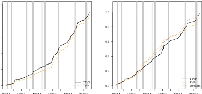
To assess how the differences in predictive accuracy evolve over time,Fig. 2displays the evolution of the cumulative log predictive Bayes factor (relative to the constant co-efficient model, left panel) and the cumulative sum of squared forecast errors (right panel) over time. It is noteworthy that LPS improvements appear to be most pro-nounced during recessions, reflecting the findings ofTable 2. During the second part of the 1990 until the midst of the 2000s, however, the relative performance of the TTVP slightly decreases vis-a-vis the TVP specification. This finding can also be seen by look-ing at the evolution of the sum of squared forecast errors, where the TTVP outperforms
errors produced by the TTVP tended to be lower as compared to a linear regression model and the TVP model. Interestingly, the point predictions of the linear model also appear to be quite competitive. This suggests that the dismal performance of the linear model almost exclusively stems from the fact that we assumed homoscedastic shocks, leading to systematically underestimated predictive intervals.
Relative LPS over time
0 1000 2000 3000 4000 5000 1957.1 1967.1 1977.1 1987.1 1997.1 2007.1 TTVP TVP
Cumulative sum of squared forecast errors over time
0.0 0.2 0.4 0.6 0.8 1.0 1957.1 1967.1 1977.1 1987.1 1997.1 2007.1 TTVP TVP constant
Fig. 2: Log predictive Bayes factor (relative to a constant coefficient model) and
cumu-lative squared forecast errors from 1947Q2 to 2010Q4. Gray shaded areas refer to US recessions dated by the NBER business cycle dating committee.
6 Empirical application II: Analyzing US monetary policy
In this section we generalize the model outlined in Section 2 to the VAR case and apply it to a typical US macroeconomic dataset.
6.1 Model specification and data
Considering anm-dimensional responseyt, let
yt=B1tyt−1+· · ·+BP tyt−P +ut, (6.1)
be a TTVP-VAR-SV model where we assume that Bpt (p = 1, . . . , P) are m× m
ma-trices of dynamic autoregressive coefficients with each element evolving according to
is distributed as
ut∼ N(0m,Σt). (6.2)
Hereby,0m denotes anm-variate zero vector andΣt =VtHtV0tdenotes a time-varying
variance-covariance matrix. The matrixVtis a lower triangular matrix with unit
diag-onal andHt=diag(eh1t, . . . , ehmt). Similar to Section 5, we assume that the logarithm
of the variances evolves according to
hit =µi+ρi(hi,t−1+µi) +νit, for i= 1, . . . , m, (6.3)
with µi and ρi being equation-specific mean and persistence parameters and νit ∼ N(0, ζi)is an equation-specific white noise error similar to the one presented in Section
5. For the covariances in Vt we impose the random walk state equation with errors
given byEq. (2.3).
Conditional on the ordering of the variables it is straightforward to estimate the TTVP model on an equation-by-equation basis, augmenting the ith equation with the contemporaneous values of the preceeding (i−1)equations (for i > 1), leading to a Cholesky-type decomposition of the variance-covariance matrix. This implies that we use the same algorithm as in Section 5, simulating each equation simultaneously on a grid.
FollowingPrimiceri(2005), we includep= 2lags of the endogenous variables. The prior setup is similar to the one adopted in the previous sections, except that now all hyperparameters are equation specific and feature an additional index i = 1, . . . , m. More specifically, for the shrinkage part on the initial state of the system, we again set λ2i ∼ G(0.01,0.01) and ai = 0.1, and the prior on ϑij is specified to be informative
withϑ−ij1 ∼ G(3,0.03). Because our TTVP-VAR model features stochastic volatility in the errors we also have to specify suitable priors on the parameters of the state equation in the log-volatility, where we impose the same hyperparameters as in Section 4 for each equation.
The last ingredient missing is the prior on the thresholds where we set πij0 = 0.2×
max|∆βTij|and πij1 = max|∆βTij|, whereβ T
ij denotes the jth coefficient of theith row
of Bt = (B1t, . . . ,BP t). Thus, we are somewhat more informative on the lower bound
of the thresholds as compared to our simulation exercise. Again, for the off-setting constant we setκi,0j = 10−7×ϑij.
For the seven-variable VAR we draw 500 000 samples from the joint posterior and discard the first 400 000 draws as burn-in. Finally, we use thinning such that inference is based on 5000 draws out of 100 000 retained draws.
We use an extended version of the data proposed inSmets and Wouters(2003) and
on quarterly basis and comprise the log differences of consumption, investment, real GDP, hours worked, consumer prices and real wages. Last, and as a policy variable, we include the Federal Funds Rate (FFR) in levels. The monetary policy shock is cal-ibrated as a 100 basis point (bp) increase in the FFR and identified using a Cholesky ordering with the variables appearing in exactly the same order as mentioned above. This ordering is in the spirit ofChristiano, Eichenbaum, and Evans(2005) and has been subsequentially used extensively in the literature (see Coibion, 2012, for an excellent survey).
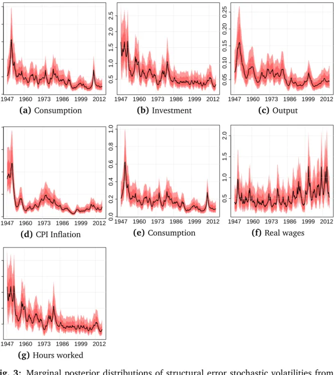
6.2 Volatility of structural shocks
Before proceeding to the dynamic responses of the macroeconomy with respect to a monetary policy shock,Fig. 3depicts the posterior distribution of the stochastic volatil-ities for all variables in our model (with dark red areas representing the 68% credible set).
As compared to previous studies who often rely on a pre-sample to tune the priors used in the state equation, our approach takes advantage of the full dataset since no psample tuning is required. Looking at the evolution of macroeconomic volatility re-veals that for almost all quantities under scrutiny, volatility decreased markedly during the 1950s. The only exception proves to be the volatility of the monetary policy shock, which peaks during the reign of Paul Volcker, who sharply increased short-term interest rates to levels above 13 percent. For all remaining shocks, the sharp spike in volatility during the first few years dwarfs other spikes, including the high inflation period dur-ing the midst of the 1970s, different economic and financial crises (most notably the global financial crisis in 2008) and other geopolitical events like the oil price shocks in the beginning and towards the end of the 1970s. Apart from the longer time span we are able to consider, the pattern remains similar to established findings in the literature (see, for instance,Primiceri,2005;Cogley and Sargent,2005).
6.3 Impulse responses to a monetary policy shock
To illustrate the usefulness of the threshold model, we examine the dynamic responses of a set of macroeconomic variables to a contractionary monetary policy shock.
Fig. 4 illustrates the effects of the monetary tightening on the real side of the econ-omy. Responses are shown after four, eight and 12 quarters with 90% (dark red) and 68% (light red) credible sets. In line with our expectations and following the monetary tightening, consumption and investment growth decelerate, driving down real output growth. Especially in the earlier part of our sample period, this decline is rather persis-tent corroborating results inChristiano, Eichenbaum, and Evans(2005). Estimates for
0.0 0.2 0.4 0.6 0.8 1.0 1947 1960 1973 1986 1999 2012 (a)Consumption 0.5 1.0 1.5 2.0 2.5 1947 1960 1973 1986 1999 2012 (b)Investment 0.05 0.10 0.15 0.20 0.25 1947 1960 1973 1986 1999 2012 (c)Output 0.0 0.5 1.0 1.5 2.0 1947 1960 1973 1986 1999 2012 (d)CPI Inflation 0.0 0.2 0.4 0.6 0.8 1.0 1947 1960 1973 1986 1999 2012 (e)Consumption 0.5 1.0 1.5 2.0 1947 1960 1973 1986 1999 2012 (f) Real wages 0.5 1.0 1.5 2.0 2.5 1947 1960 1973 1986 1999 2012 (g)Hours worked
Fig. 3: Marginal posterior distributions of structural error stochastic volatilities from
1947Q2 to 2014Q4. Dark red areas are16th and84th credible intervals and light red areas are5th and95th credible intervals. Black lines depict posterior medians.
this part of the sample imply a peak drop of real GDP of about 0.4% (in annual terms), which complies with the bulk of the literature on monetary policy that uses linear mod-els over a comparable time span (Bernanke and Blinder, 1992;Leeper, Sims, and Zha,
1996;Uhlig,2005).
As is evident from Fig. 4, we find a lot of variation in the parameters and conse-quently impulse response functions. For example, the effects of a (hypothetical) mone-tary policy shock on consumption and investment would have been about twice as high during the Bretton Woods period (1951 to 1971), compared to the period of the Great Inflation (1971 to 1983, seeD’Agostino and Surico,2012, for a systematic categoriza-tion of monetary regimes in the USA). After the period of the Great Inflacategoriza-tion these ef-fects diminish even further. This corroborates findings of Boivin and Giannoni(2006), who provide evidence for a reduced effect of monetary policy shocks in the post-1980 period. This time pattern directly carries over to effects on output growth, implying that the inflationary environment at the time a shock hits the economy plays an important role in determining the size of the macroeconomic responses. Further time variation is evident when looking at the 12 quarter forecast horizon: In the medium-term, effects on investment, consumer price and output growth increase considerably with the out-break of the global financial crisis 2008. Taken at face value, this suggests that after a prolonged period of unaltered interest rates, a deviation from the (long-run) inter-est rate mean, can exert considerable effects on the macroeconomy. This result is in line with Feldkircher and Huber (2016) who use a standard time-varying parameter VAR model with stochastic volatility to investigate changes in the US monetary policy transmission channel.
Fig. 5 shows the results for the remaining variables, hours worked as a proxy for capital utilization, real wages and the FFR itself.
The monetary tightening decreases hours worked throughout the sample period and at all forecast horizons considered. In line with our previous results, the size of the effects vary over the sample period: effects are least pronounced during the Great Inflation and Great Moderation period and longer-term responses considerably increase after the global financial crisis. A different pattern emerges for real wages. Here, responses can be broadly categorized into two regimes, a pre-Great-Inflation-period and a post-Great-Inflation regime. In the former, responses are negative, implying that a monetary tightening has a detrimental effect on real wage growth, which is tightly estimated up to eight quarters. During the Great Inflation period, effects become less pronounced and start turning positive. Finally, in the post-Great-Inflation period, effects are positive, but credible sets are considerably wide. Last, responses of short-term interest rates stay elevated up until 12 quarters, after which credible sets become wide.
Consumption 1947 1954 1960 1966 1972 1979 1985 1991 1997 2004 2010 −1.5 −1.0 −0.5 0.0 In vestment 1947 1954 1960 1966 1972 1979 1985 1991 1997 2004 2010 −0.20 −0.15 −0.10 −0.05 0.00 0.05 Output 1947 1954 1960 1966 1972 1979 1985 1991 1997 2004 2010 −0.15 −0.10 −0.05 0.00 0.05 0.10 Inflation 1947 1954 1960 1966 1972 1979 1985 1991 1997 2004 2010 1947 1954 1960 1966 1972 1979 1985 1991 1997 2004 2010 −1.5 −1.0 −0.5 0.0 1947 1954 1960 1966 1972 1979 1985 1991 1997 2004 2010 −0.20 −0.15 −0.10 −0.05 0.00 0.05 1947 1954 1960 1966 1972 1979 1985 1991 1997 2004 2010 −0.15 −0.10 −0.05 0.00 0.05 0.10 1947 1954 1960 1966 1972 1979 1985 1991 1997 2004 2010 1947 1954 1960 1966 1972 1979 1985 1991 1997 2004 2010 −1.5 −1.0 −0.5 0.0 1947 1954 1960 1966 1972 1979 1985 1991 1997 2004 2010 −0.20 −0.15 −0.10 −0.05 0.00 0.05 1947 1954 1960 1966 1972 1979 1985 1991 1997 2004 2010 −0.15 −0.10 −0.05 0.00 0.05 0.10 1947 1954 1960 1966 1972 1979 1985 1991 1997 2004 2010 ig. 4: P osterior median responses to a +100 bp monetary policy shock, after 4 (top panels), 8 (middle panels) and 12 (bottom panels) quarters. Shaded areas correspond to 90% (dark red) and 68% (light red) credible sets.
−0.3 −0.2 −0.1 0.0 Hour s w orked 1947 1952 1956 1961 1965 1970 1974 1979 1983 1988 1992 1997 2001 2006 2010 t= 4 −0.4 −0.2 0.0 0.2 0.4 0.6 Real wa g es 1947 1952 1956 1961 1965 1970 1974 1979 1983 1988 1992 1997 2001 2006 2010 0.0 0.5 1.0 1.5 2.0
Federal funds rate
1947 1952 1956 1961 1965 1970 1974 1979 1983 1988 1992 1997 2001 2006 2010 −0.3 −0.2 −0.1 0.0 1947 1952 1956 1961 1965 1970 1974 1979 1983 1988 1992 1997 2001 2006 2010 t= 8 −0.4 −0.2 0.0 0.2 0.4 0.6 1947 1952 1956 1961 1965 1970 1974 1979 1983 1988 1992 1997 2001 2006 2010 0.0 0.5 1.0 1.5 2.0 1947 1952 1956 1961 1965 1970 1974 1979 1983 1988 1992 1997 2001 2006 2010 −0.3 −0.2 −0.1 0.0 1947 1952 1956 1961 1965 1970 1974 1979 1983 1988 1992 1997 2001 2006 2010 t= 12 −0.4 −0.2 0.0 0.2 0.4 0.6 1947 1952 1956 1961 1965 1970 1974 1979 1983 1988 1992 1997 2001 2006 2010 0.0 0.5 1.0 1.5 2.0 1947 1952 1956 1961 1965 1970 1974 1979 1983 1988 1992 1997 2001 2006 2010 F ig. 5: P osterior median responses to a +100 bp monetary policy shock, after 4 (top panels), 8 (middle panels) and 12 (bottom panels) quarters. Shaded areas correspond to 90% (dark red) and 68% (light red) credible sets.
Again, there is a considerable increase in the size of the response after 2008 and – in contrast to responses of other variables – throughout all forecast horizons considered.
7 Closing remarks
This paper puts forth a novel approach to estimate time-varying parameter models in a Bayesian framework. We assume that the state innovations are following a threshold model where the threshold variable is the absolute period-on-period change of the cor-responding states. This implies that if the (proposed) change is sufficiently large, the corresponding variance is set to a value greater than zero, and zero otherwise, which implies that the states remained constant from (t−1)to t. Our framework is capable of discriminating between a plethora of competing specifications, most notably models that feature a large, moderate and low number of structural breaks in the regression parameters. In a simulation study we assess under which circumstances our modeling framework performs particularly well, assuming a large number of possible data gen-erating processes. Using a well known dataset we predict the S&P 500 excess return using our framework and benchmark it against two nested alternatives. We find that the TTVP model yields more precise density forecasts while the quality of point forecasts is similar to an unrestricted TVP when the full sample is taken under consideration. Last, we generalize our model to the time-varying VAR framework with stochastic volatility and investigate responses to a contractionary monetary policy shock. Our results show that effects of the monetary policy shock vary considerably over time and in a way that can be rationalized by US monetary and economic history. More specifically, most vari-ables respond strongest in the early part of the sample, while monetary policy shocks become less effective thereafter (Boivin and Giannoni, 2006). Especially during the Great Moderation effects are rather modest and stable over time. This changes with the outbreak of the global financial crisis, which boosts effects of monetary policy on a range of different variables.
References
ANG, A., AND G. BEKAERT (2007): “Stock return predictability: Is it there?,”Review of Financial studies, 20(3), 651–707.
BELMONTE, M. A., G. KOOP, AND D. KOROBILIS (2014): “Hierarchical Shrinkage in
Time-Varying Parameter Models,” Journal of Forecasting, 33(1), 80–94.
BERNANKE, B. S., AND A. S. BLINDER (1992): “The Federal Funds Rate and the
Chan-nels of Monetary Transmission,”American Economic Review, 82(4), 901–21.
BITTO, A., AND S. FRUHWIRTH¨ -SCHNATTER (2015): “Achieving shrinkage in the
Workshop on Statistical Modelling, Volume 2, ed. by H. Friedl, and H. Wagner, pp. 43–46, Linz, Austria.
BOIVIN, J., AND M. P. GIANNONI (2006): “Has Monetary Policy Become More
Effec-tive?,”The Review of Economics and Statistics, 88(3), 445–462.
CARTER, C. K., AND R. KOHN (1994): “On Gibbs sampling for state space models,”
Biometrika, 81(3), 541–553.
CHRISTIANO, L. J., M. EICHENBAUM, AND C. L. EVANS(2005): “Nominal Rigidities and the Dynamic Effects of a Shock to Monetary Policy,” Journal of Political Economy, 113(1), 1–45.
CLARK, T. E. (2012): “Real-time density forecasts from Bayesian vector autoregressions with stochastic volatility,”Journal of Business & Economic Statistics.
CLARK, T. E.,ANDF. RAVAZZOLO(2015): “Macroeconomic Forecasting Performance
un-der Alternative Specifications of Time-Varying Volatility,” Journal of Applied Econo-metrics, 30(4), 551–575.
COGLEY, T., AND T. J. SARGENT (2002): “Evolving post-world war II US inflation
dy-namics,” inNBER Macroeconomics Annual 2001, Volume 16, pp. 331–388. MIT Press. (2005): “Drifts and volatilities: monetary policies and outcomes in the post WWII US,”Review of Economic Dynamics, 8(2), 262–302.
COIBION, O. (2012): “Are the Effects of Monetary Policy Shocks Big or Small?,” Ameri-can Economic Journal: Macroeconomics, 4(2), 1–32.
D’AGOSTINO, A., L. GAMBETTI,ANDD. GIANNONE(2013): “Macroeconomic forecasting
and structural change,”Journal of Applied Econometrics, 28(1), 82–101.
D’AGOSTINO, A., AND P. SURICO(2012): “A Century of Inflation Forecasts,” The Review of Economics and Statistics, 94(4), 1097–1106.
DANGL, T., AND M. HALLING (2012): “Predictive regressions with time-varying coeffi-cients,” Journal of Financial Economics, 106(1), 157–181.
EISENSTAT, E., J. C. CHAN, AND R. W. STRACHAN (2016): “Stochastic model
specifica-tion search for time-varying parameter VARs,”Econometric Reviews, pp. 1–28.
FELDKIRCHER, M., AND F. HUBER (2016): “Unconventional US Monetary Policy: New
Tools, Same Channels?,” Working Papers 208, Oesterreichische Nationalbank (Aus-trian Central Bank).
FRUHWIRTH¨ -SCHNATTER, S. (1994): “Data augmentation and dynamic linear models,”
Journal of time series analysis, 15(2), 183–202.
FRUHWIRTH¨ -SCHNATTER, S., AND H. WAGNER (2010): “Stochastic model specification search for Gaussian and partial non-Gaussian state space models,”Journal of Econo-metrics, 154(1), 85–100.
GERLACH, R., C. CARTER, AND R. KOHN (2000): “Efficient Bayesian inference for dy-namic mixture models,” Journal of the American Statistical Association, 95(451), 819–828.
GEWEKE, J., AND G. AMISANO (2010): “Comparing and evaluating Bayesian predictive
distributions of asset returns,”International Journal of Forecasting, 26(2), 216–230. (2012): “Prediction with misspecified models,” The American Economic Review, 102(3), 482–486.
GIORDANI, P., AND R. KOHN (2012): “Efficient Bayesian inference for multiple
change-point and mixture innovation models,”Journal of Business & Economic Statistics.
GRIFFIN, J. E., AND P. J. BROWN (2010): “Inference with normal-gamma prior
H¨ORMANN, W., AND J. LEYDOLD (2013): “Generating generalized inverse Gaussian random variates,”Statistics and Computing, 24(4), 1–11.
KALLI, M., AND J. E. GRIFFIN (2014): “Time-varying sparsity in dynamic regression
models,”Journal of Econometrics, 178(2), 779–793.
KASTNER, G. (2016): “Dealing with stochastic volatility in time series using the R
pack-age stochvol,”Journal of Statistical Software, 69(5), 1–30.
KASTNER, G., AND S. FR¨UHWIRTH-SCHNATTER (2014): “Ancillarity-sufficiency inter-weaving strategy (ASIS) for boosting MCMC estimation of stochastic volatility mod-els,” Computational Statistics & Data Analysis, 76, 408–423.
KIMURA, T., AND J. NAKAJIMA (2016): “Identifying conventional and unconventional
monetary policy shocks: a latent threshold approach,”The BE Journal of Macroeco-nomics, 16(1), 277–300.
KOOP, G., AND D. KOROBILIS(2012): “Forecasting inflation using dynamic model aver-aging,” International Economic Review, 53(3), 867–886.
(2013): “Large time-varying parameter VARs,”Journal of Econometrics, 177(2), 185–198.
KOOP, G., R. LEON-GONZALEZ, AND R. W. STRACHAN (2009): “On the evolution of
the monetary policy transmission mechanism,” Journal of Economic Dynamics and Control, 33(4), 997–1017.
KOOP, G., AND S. M. POTTER (2007): “Estimation and forecasting in models with
mul-tiple breaks,”The Review of Economic Studies, 74(3), 763–789.
LEEPER, E. M., C. A. SIMS, AND T. ZHA (1996): “What Does Monetary Policy Do?,”
Brookings Papers on Economic Activity, 27(2), 1–78.
LETTAU, M., AND S. LUDVIGSON (2001): “Consumption, aggregate wealth, and
ex-pected stock returns,”the Journal of Finance, 56(3), 815–849.
LEYDOLD, J., AND W. H¨ORMANN (2015): GIGrvg: Random variate generator for the GIG
distributionR package version 0.4.
MCCULLOCH, R. E., AND R. S. TSAY (1993): “Bayesian inference and prediction for
mean and variance shifts in autoregressive time series,” Journal of the American Statistical Association, 88(423), 968–978.
NAKAJIMA, J., AND M. WEST (2013a): “Bayesian analysis of latent threshold dynamic
models,”Journal of Business & Economic Statistics, 31(2), 151–164.
(2013b): “Dynamic factor volatility modeling: A Bayesian latent threshold approach,”Journal of Financial Econometrics, 11(1), 116–153.
POLK, C., S. THOMPSON, AND T. VUOLTEENAHO (2006): “Cross-sectional forecasts of
the equity premium,”Journal of Financial Economics, 81(1), 101–141.
PRIMICERI, G. E. (2005): “Time varying structural vector autoregressions and
mone-tary policy,”The Review of Economic Studies, 72(3), 821–852.
RITTER, C.,AND M. A. TANNER(1992): “Facilitating the Gibbs sampler: the Gibbs
stop-per and the griddy-Gibbs sampler,” Journal of the American Statistical Association, 87(419), 861–868.
SIMS, C. A., ANDT. ZHA(2006): “Were there regime switches in US monetary policy?,” The American Economic Review, pp. 54–81.
SMETS, F., AND R. WOUTERS (2003): “An estimated dynamic stochastic general
equi-librium model of the euro area,”Journal of the European economic association, 1(5), 1123–1175.
macroeconomic time series relations,” Journal of Business & Economic Statistics, 14(1), 11–30.
UHLIG, H. (2005): “What are the effects of monetary policy on output? Results from an
agnostic identification procedure,”Journal of Monetary Economics, 52(2), 381–419. WELCH, I., AND A. GOYAL(2008): “A comprehensive look at the empirical performance
of equity premium prediction,”Review of Financial Studies, 21(4), 1455–1508. ZHOU, X., J. NAKAJIMA, AND M. WEST (2014): “Bayesian forecasting and portfolio
decisions using dynamic dependent sparse factor models,” International Journal of Forecasting, 30(4), 963–980.