A Comparative Study of Simple Online Learning Strategies for
Streaming Data
M. MILL ´AN-GIRALDO J. S. S ´ANCHEZ
Universitat Jaume I
Dept. Llenguatges i Sistemes Inform´atics Av. Sos Baynat s/n, 12071 Castell´o de la Plana
SPAIN
{mmillan,sanchez}@uji.es
Abstract:Since several years ago, the analysis of data streams has attracted considerably the attention in various research fields, such as databases systems and data mining. The continuous increase in volume of data and the high speed that they arrive to the systems challenge the computing systems to store, process and transmit. Furthermore, it has caused the development of new online learning strategies capable to predict the behavior of the streaming data. This paper compares three very simple learning methods applied to static data streams when we use the 1-Nearest Neighbor classifier, a linear discriminant, a quadratic classifier, a decision tree, and the Na¨ıve Bayes classifier. The three strategies have been taken from the literature. One of them includes a time-weighted strategy to remove obsolete objects from the reference set. The experiments were carried out on twelve real data sets. The aim of this experimental study is to establish the most suitable online learning model according to the performance of each classifier.
Key–Words:Data mining, Online learning, Static streaming data, Forgetting
1 Introduction
Classification is one of the key tasks in many pattern recognition and data mining applications. The essence of classification is to use previously observed data to construct a model that is able to predict the categorical or nominal value of a dependent variable (the class) given the values of the independent variables (the fea-tures or attributes). Obtaining a high accuracy in clas-sification is usually the primary goal. Another impor-tant objective is comprehensibility, which refers to the ability of a human expert to understand the classifica-tion model. The third aim is compactness, which re-lates to the size of the model. Classifiers usually try to trade-off these three objectives.
Most traditional learning algorithms assume the availability of a set of labelled (training) examples
T = {e1, e2, . . . , en}. Each training exampleei is a
pair formed by a feature vector−→xi and a discrete value
yi (class label) taken from a finite setY. In many
domains, however, collecting labelled training objects may be costly, time-consuming or even dangerous, while it is relatively easy to obtain unlabelled ob-jects. This has provoked significant interest in semi-supervised learning [3] and other closely related areas as incremental learning, online learning and stream-ing data. In [8], a neural network is employed to learn temporal patterns incrementally using Gaussian
func-tions and chunking to group similar patterns. On the
other hand, Gayar et al.[6] suggest a new technique
for semi-supervised learning with multiple classifier systems in face recognition, that combines co-training and self-supervised learning.
In a growing number of real applications, the data are not available as a batch but comes one object at
a time (called streaming data). From the
process-ing point of view, a data stream is an infinite flow of highly rapid generated objects that challenge our computing systems to store, process and transmit [10]. Examples of applications with data streams include Internet peer-to-peer downloads and multimedia [7], radar derived meteorological data, banking and credit transactions, classification of stock data, and intrusion detection in computer networks, for which it is not possible to collect all relevant input data before us-ing the classification algorithm. Under these circum-stances, the learning systems have to operate
contin-uously (online systems) and process each data item in
near-real time.
It has been argued that a good online classifier should have the following characteristics [4, 5, 15]:
(i) Single pass through the data: the classifier must be able to learn from each data point without re-visiting it.
(ii) Limited memory and processing time: each data point should be processed in a constant time re-gardless of the number of points processed in the past.
(iii) Any-time-learning: if stopped at timet, the
cur-rent classifier should be equivalent to a classifier
trained on the batch data up to timet.
These are also valid for online learning of
stream-ing data, but yet another desiderata is generally
ac-cepted for this: At any timetin the data stream, we
would like the per-item processing time, storage as
well as the computing time to be simultaneouslyo(N;
t), beingN the number of data items processed.
The focus of this paper is on evaluating sev-eral simple strategies for online versions of tradi-tional learning algorithms applied to static streaming data. We empirically compare three existing strategies taken from the literature when applied to the 1-Nearest Neighbor classifier, a linear discriminant, a quadratic classifier, a decision tree, and the Na¨ıve Bayes clas-sifier. The aim of this experimental study is to con-clude the most appropriate online learning model for streaming data.
2 Strategies for Online Learning
One of the most important decisions in designing an online classifier is how to maintain the reference set. The three trivial possibilities with respect to the mem-ory size are [9]:
1. Full memory, in which the learner retains all training objects.
2. Partial memory, in which it retains only some of the training objects.
3. No memory, in which it retains none.
Some online classifiers where stored examples are used directly to form predictions should be in the partial memory group. Ideally, we need to keep a (small) reference set which, when deemed necessary, is expanded or shrunk within given limits. This means that there must be some mechanism to forget (remove) objects. How to forget is a difficult problem that can be tackled through several strategies.
• Passive forgetting [12] (also called time-weighted forgetting [14] and implicit forget-ting [5, 14]) is based only on the time elapsed since the object was added to the reference set. It assumes that the importance of data decreases over time. Passive forgetting acts as a moving
window where the reference set is the last data batch. Its size is a parameter of the algorithm.
• Active forgetting[12] (also referred as to explicit forgetting [5, 14]) implies that more information from data is used to decide which objects should be dropped. Two alternatives are possible for ac-tive forgetting:
(i) Density-based forgetting follows the intu-ition of the “life” game. If a region is too crowded, we sieve out some objects (locally-weighted forgetting [14]). On the other hand, if a region is too distant, and not providing nearest neighbors, it is re-moved altogether [14]. In the jargon of data editing, the former strategy corresponds to condensing, while the latter corresponds to editing.
(ii) Error-based forgetting is perceived as the most successful of the forgetting heuris-tics [1, 12, 14]. In this case, each object in the reference set has a classification record. The more streaming data it labels correctly, the stronger its record becomes. The ob-jects with weak records are cleared at regu-lar intervals.
2.1 The models for the experiment
The first strategy we will here experiment with is a full memory model, in which all new objects have to be incorporated into the reference set. The other two lie in the group of partial memory, that is, only some new objects will be added to the reference set. In the case of partial memory, one model employs a passive forgetting strategy in order to remove ”obsolete” ex-amples from the reference set.
1. All, which corresponds to the full memory
op-tion. It assumes that all new examples are valid and equally important. It is clear that the use of this model may result in a huge reference set, making impossible its practical application in most real problems.
2. Every n objects, in which everyn’th object will be added to the reference set to retrain the clas-sifier. It considers that the ’All’ strategy will re-train too often. On the other hand, this model overcomes the storage problem of the ’All’ ap-proach.
3. Window of fixed size. The reference set will be of fixed size with the last data, assuming that the most relevant information is at the last processed
objects. Besides, the a priori class distributions are kept for each reference set in order to avoid a class to be emptied.
Although very simple strategies for online learn-ing, they will allow to compare the partial memory and full memory approaches in a static streaming data scenario.
3 Experiments
In this section we present the experiments carried out in order to compare the simple online learning strate-gies previously described. The aim of this empirical study is to analyze the behavior of each pair (online learning strategy, classifier).
3.1 The data sets
Twelve real data sets were employed in the present experiment (a summary can be seen in Table 1). Data
were normalized in the range[0,+1]. All features
(at-tributes) were numerical and there were no missing values.
Table 1: Characteristics of the real data sets used in the experiment
Data set Features Classes Objects Source
iris 4 3 150 UCI1 wine 13 3 178 UCI crabs 6 2 200 Ripley2 sonar 60 2 208 UCI thyroid 5 3 215 UCI wbc 30 2 569 UCI breast 9 2 277 UCI intubation 17 2 302 Library liver 6 2 345 UCI spect 44 2 349 Library laryngeal3 16 3 353 Library australian 42 2 690 UCI 1UCI [2] 2Ripley [13] 3Library http://www.informatics.bangor.ac.uk/
∼kuncheva/activities/real data full set.htm
Although there is no strict guideline about what a sufficient data size is, the common wisdom [11] is that the size of the training data should be around
10 ×d×c, where d is the number of features and
c is the number of classes in a problem. Our small
initial reference set was of size1×d×c.
The experimental set-up was as follows:
• 100 runs were carried out with 90% of the data
used for training and 10% used for testing. The splits were done using stratified sampling.
• From each training part of the data, a random
stratified sample ofNl = 1×n×cwas taken
as the initial labelled references set.
• The remaining part of the training data was used
as the new coming online data. To simulate an i.i.d. sequence, the data was shuffled before each of the 100 runs.
• One point from the online data was fed to the
sys-tem at a time. The point was processed according to the respective strategy to handle online learn-ing. The classification error was evaluated on the testing set. In this way we created a “progression curve” which is the classification error as a func-tion of the number of online objects seen by the classifier.
• The results were averaged across the 100 runs,
giving a single progression curve for each data set.
The strategies we compare through this experi-ment are those introduced in Section 2, that is, ’All’,
’Every n objects’ (n = 5), and ’Window of fixed
size’ (equal to the original size). All these have
been applied to five different classifiers: the 1-Nearest Neighbor classifier (1-NN), a linear discriminant, a quadratic classifier, a decision tree (DT), and the Na¨ıve Bayes classifier.
For each of the 100 runs of the experiment, all methods received the same partitions of the data into initial, online and testing sets. The online (unlabelled) data were presented to all strategies in the same order.
3.2 The results
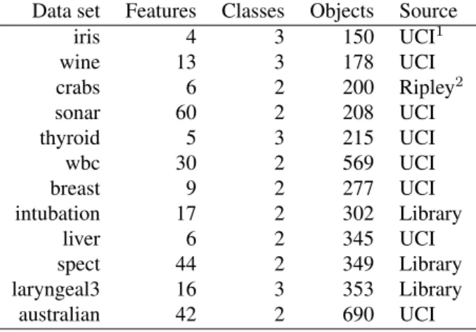
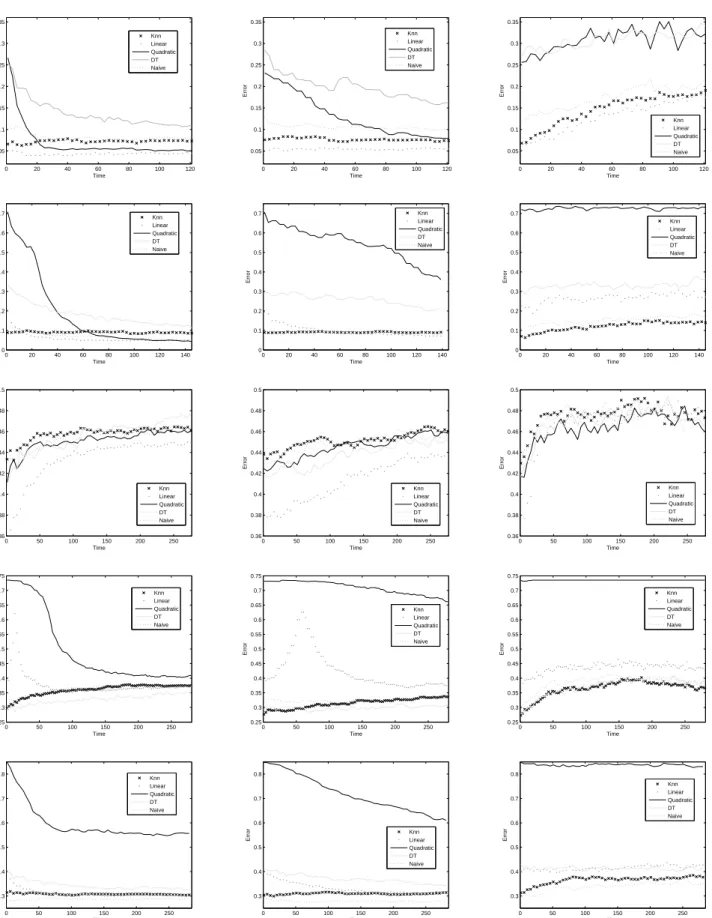
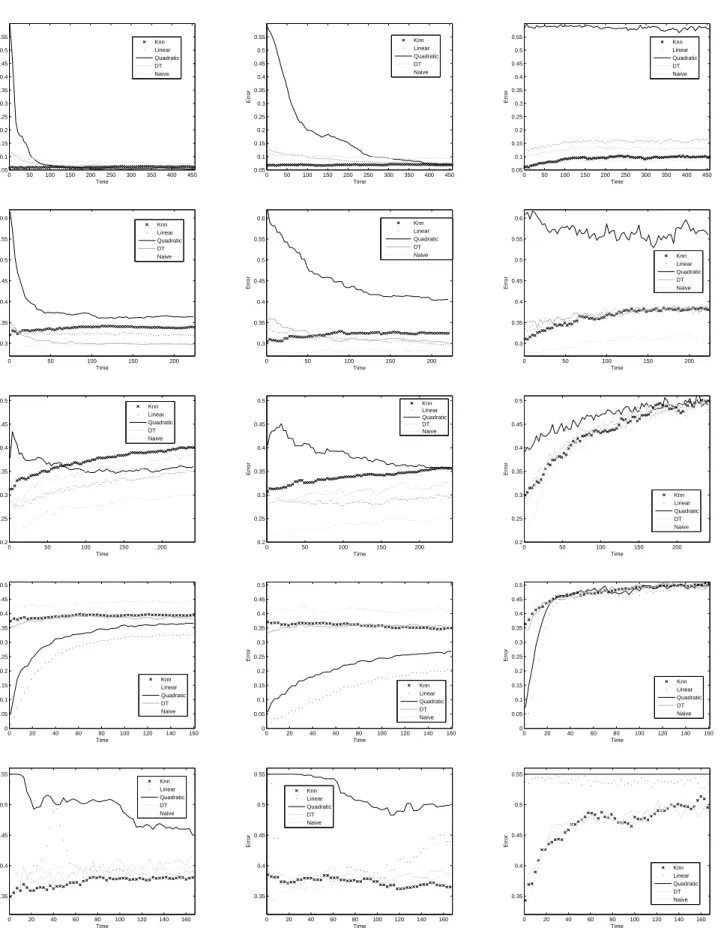
The results for the iris, wine, liver, spect, laryngeal3, and wbc are displayed in Figure 1, whereas those for breast, intubation, crabs, and sonar are in Fig-ure 2, and the results for thyroid and australian are in Figure 3. The x-axis corresponds to the number of processed unlabelled samples and the y-axis is the progression of the classification error, evaluated on the testing sets and averaged across 100 runs.
The graphs are especially meant to visualize the direction of the error curves rather than the details. From these, several typical patterns can be observed. The error rates have different trends when
compar-ing the ’All’ and ’Everynobjects’ strategies with the
’Window of fixed size’ approach. While using the
in error as more unlabelled samples are processed, the third model produces the opposite effect.
Probably, the degradation of the window-based approach is mainly due to the fact that the reference set is gradually updated with new objects labelled by the own classifier; if this errs, then misclassified ob-jects will be added to the reference set. As stated in Section 2, passive forgetting is based only on the time elapsed since the object was added to the ref-erence set. This means that no test will be used to evaluate the goodness of each new object labelled and consequently, noise and errors may be incorporated into the reference set. Thus the quality of the refer-ence set gradually deteriorates with more unlabelled objects being processed.
The quadratic classifier clearly shows the behav-ior just described. Contrary to the case of the
window-based model, the ’All’ and ’Every n objects’
strate-gies start from a high error rate, but this rapidly de-creases with processing of new objects. This pattern, however, is not matched on all data sets. There are two databases (liver and crabs) where the errors of the quadratic classifier increase with the processing
of new samples by means of the ’All’ and ’Everyn
objects’ approaches.
Although the general behavior of the rest of clas-sifiers is similar to that of the quadratic, it worths pointing out that the error rates of 1-NN, the linear discriminant, the decision tree, and the Na¨ıve Bayes classifier keep quite steady along time in the case of
the ’All’ and ’Everynobjects’ models. It seems that
in general, small changes in the reference set do not strongly affect the classifier performance. Neverthe-less, when the whole set is updated as a result of the forgetting mechanism, it produces a significant degra-dation in performance.
The results described above have been corrobo-rated by comparing the error rates of each model at
the initial time t0 and at the final timetf, when all
the streaming data have already been seen. The er-ror rates obtained are included in Tables 2, 3 and 4,
for each strategy ’All’, ’Everynobjects’, and
’Win-dow of fixed size’, respectively. From these tables, we could obtain more detailed information.
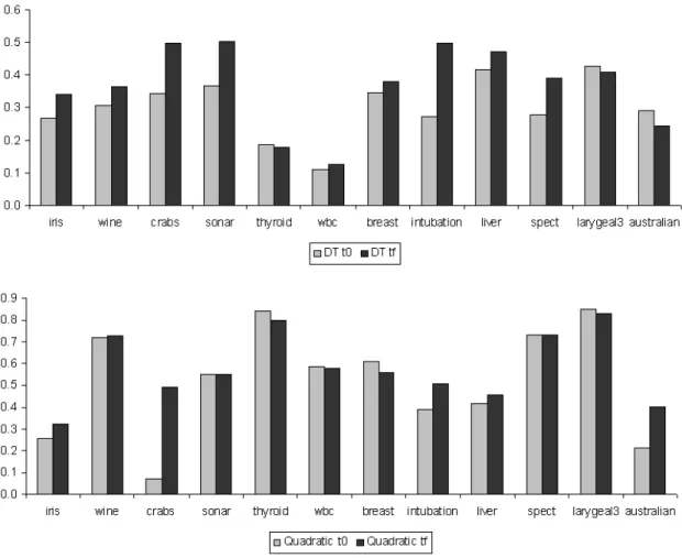
In the ’All’ and ’Everynobjects’ approaches, the
1-Nearest Neighbor and Na¨ıve Bayes classifiers are the most constant, because they do not show signif-icant changes compared with the rest of classifiers. However, in most cases for both classifiers, the final error rate is higher than the initial error rate.
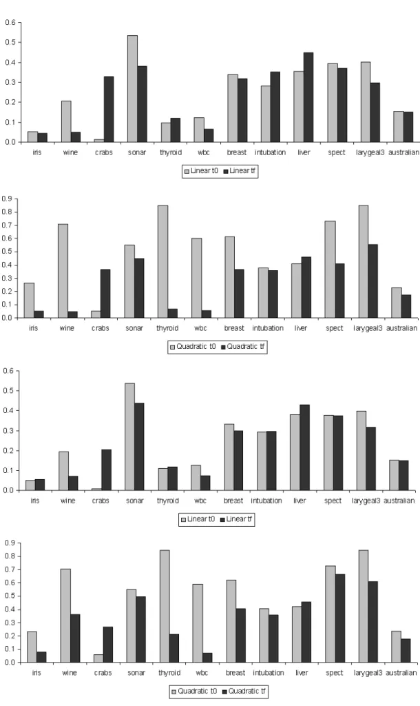
Otherwise, for linear and quadratic classifiers in
the ’All’ and ’Every n objects’ strategies, in most
cases the error decreases as more unlabelled objects are processed (Figure 4). The error rate for the deci-sion tree with the ’All’ approach increases on the half
of the databases, whereas for the rest there occurs the opposite effect, as can be observed in Figure 5. On
the other hand, in the ’Everynobjects’ model the
de-cision tree behavior is similar to that of the linear and quadratic classifiers.
In the ’Window of fixed size’ strategy, as already mentioned, the error rate increases for all the classifi-cation models except for the quadratic classifier with the breast and thyroid data sets, and for the decision tree with the australian and laryngeal3 data sets (see Figure 6).
4 Conclusions and Further
Exten-sions
In this paper, we have compared a number of simple strategies for online learning of streaming data. Two models belong to the group of partial memory (only some new objects are retained in the reference set), whereas the third is a full memory method (all new un-labelled samples are kept). Besides, one of the partial memory models includes a time-weighted forgetting strategy in order to remove ”obsolete” objects from the reference set.
The empirical study has employed five classifiers with very different properties so that one can con-clude which strategy is more suitable for each learn-ing model. The experiments have shown that the error rates of the ’Window of fixed size’ (partial memory with passive forgetting) approach increases with the processing of new samples, suggesting that a drastic update of the reference set may significantly deteri-orate the classifier performance. From the results, it can be concluded that the inclusion of some forget-ting mechanism will be especially useful in the case of non-stationary data streams.
Future work will focus on a more exhaustive study of a larger number of strategies for online learn-ing, especially addressed to devise more elaborated forgetting methods. Another topic for further study will be to determine the optimal number of training examples to keep in the reference set. Also, extend-ing the present study to dynamic streamextend-ing data con-stitutes one of the most important lines for future re-search.
Acknowledgements: This work has been supported in part by the Spanish Ministry of Education and Sci-ence under grants DPI2006–15542 and CSD2007– 00018 (Consolider–Ingenio 2010).
0 20 40 60 80 100 120 0.05 0.1 0.15 0.2 0.25 0.3 0.35 Time Error Knn Linear Quadratic DT Naive 0 20 40 60 80 100 120 0.05 0.1 0.15 0.2 0.25 0.3 0.35 Time Error Knn Linear Quadratic DT Naive 0 20 40 60 80 100 120 0.05 0.1 0.15 0.2 0.25 0.3 0.35 Time Error Knn Linear Quadratic DT Naive 0 20 40 60 80 100 120 140 0 0.1 0.2 0.3 0.4 0.5 0.6 0.7 Time Error Knn Linear Quadratic DT Naive 0 20 40 60 80 100 120 140 0 0.1 0.2 0.3 0.4 0.5 0.6 0.7 Time Error Knn Linear Quadratic DT Naive 0 20 40 60 80 100 120 140 0 0.1 0.2 0.3 0.4 0.5 0.6 0.7 Time Error Knn Linear Quadratic DT Naive 0 50 100 150 200 250 0.36 0.38 0.4 0.42 0.44 0.46 0.48 0.5 Time Error Knn Linear Quadratic DT Naive 0 50 100 150 200 250 0.36 0.38 0.4 0.42 0.44 0.46 0.48 0.5 Time Error Knn Linear Quadratic DT Naive 0 50 100 150 200 250 0.36 0.38 0.4 0.42 0.44 0.46 0.48 0.5 Time Error Knn Linear Quadratic DT Naive 0 50 100 150 200 250 0.25 0.3 0.35 0.4 0.45 0.5 0.55 0.6 0.65 0.7 0.75 Time Error Knn Linear Quadratic DT Naive 0 50 100 150 200 250 0.25 0.3 0.35 0.4 0.45 0.5 0.55 0.6 0.65 0.7 0.75 Time Error Knn Linear Quadratic DT Naive 0 50 100 150 200 250 0.25 0.3 0.35 0.4 0.45 0.5 0.55 0.6 0.65 0.7 0.75 Time Error Knn Linear Quadratic DT Naive 0 50 100 150 200 250 0.3 0.4 0.5 0.6 0.7 0.8 Time Error Knn Linear Quadratic DT Naive 0 50 100 150 200 250 0.3 0.4 0.5 0.6 0.7 0.8 Time Error Knn Linear Quadratic DT Naive 0 50 100 150 200 250 0.3 0.4 0.5 0.6 0.7 0.8 Time Error Knn Linear Quadratic DT Naive
Figure 1: Error progression with sequential processing of new unlabelled data through the three online learning
strategies: ’All’ (left), ’Everyn= 5objects’ (middle), and ’Window of fixed size’ (right). From top to bottom, the
0 50 100 150 200 250 300 350 400 450 0.05 0.1 0.15 0.2 0.25 0.3 0.35 0.4 0.45 0.5 0.55 Time Error Knn Linear Quadratic DT Naive 0 50 100 150 200 250 300 350 400 450 0.05 0.1 0.15 0.2 0.25 0.3 0.35 0.4 0.45 0.5 0.55 Time Error Knn Linear Quadratic DT Naive 0 50 100 150 200 250 300 350 400 450 0.05 0.1 0.15 0.2 0.25 0.3 0.35 0.4 0.45 0.5 0.55 Time Error Knn Linear Quadratic DT Naive 0 50 100 150 200 0.3 0.35 0.4 0.45 0.5 0.55 0.6 Time Error Knn Linear Quadratic DT Naive 0 50 100 150 200 0.3 0.35 0.4 0.45 0.5 0.55 0.6 Time Error Knn Linear Quadratic DT Naive 0 50 100 150 200 0.3 0.35 0.4 0.45 0.5 0.55 0.6 Time Error Knn Linear Quadratic DT Naive 0 50 100 150 200 0.2 0.25 0.3 0.35 0.4 0.45 0.5 Time Error Knn Linear Quadratic DT Naive 0 50 100 150 200 0.2 0.25 0.3 0.35 0.4 0.45 0.5 Time Error Knn Linear Quadratic DT Naive 0 50 100 150 200 0.2 0.25 0.3 0.35 0.4 0.45 0.5 Time Error Knn Linear Quadratic DT Naive 0 20 40 60 80 100 120 140 160 0 0.05 0.1 0.15 0.2 0.25 0.3 0.35 0.4 0.45 0.5 Time Error Knn Linear Quadratic DT Naive 0 20 40 60 80 100 120 140 160 0 0.05 0.1 0.15 0.2 0.25 0.3 0.35 0.4 0.45 0.5 Time Error Knn Linear Quadratic DT Naive 0 20 40 60 80 100 120 140 160 0 0.05 0.1 0.15 0.2 0.25 0.3 0.35 0.4 0.45 0.5 Time Error Knn Linear Quadratic DT Naive 0 20 40 60 80 100 120 140 160 0.35 0.4 0.45 0.5 0.55 Time Error Knn Linear Quadratic DT Naive 0 20 40 60 80 100 120 140 160 0.35 0.4 0.45 0.5 0.55 Time Error Knn Linear Quadratic DT Naive 0 20 40 60 80 100 120 140 160 0.35 0.4 0.45 0.5 0.55 Time Error Knn Linear Quadratic DT Naive
Figure 2: Error progression with sequential processing of new unlabelled data through the three online learning
strategies: ’All’ (left), ’Everyn= 5objects’ (middle), and ’Window of fixed size’ (right). From top to bottom, the
0 20 40 60 80 100 120 140 160 0.1 0.2 0.3 0.4 0.5 0.6 0.7 0.8 Time Error Knn Linear Quadratic DT Naive 0 20 40 60 80 100 120 140 160 0.1 0.2 0.3 0.4 0.5 0.6 0.7 0.8 Time Error Knn Linear Quadratic DT Naive 0 20 40 60 80 100 120 140 160 0.1 0.2 0.3 0.4 0.5 0.6 0.7 0.8 Time Error Knn Linear Quadratic DT Naive 0 100 200 300 400 500 0.15 0.2 0.25 0.3 0.35 0.4 Time Error Knn Linear Quadratic DT Naive 0 100 200 300 400 500 0.15 0.2 0.25 0.3 0.35 0.4 Time Error Knn Linear Quadratic DT Naive 0 100 200 300 400 500 0.15 0.2 0.25 0.3 0.35 0.4 Time Error Knn Linear Quadratic DT Naive
Figure 3: Error progression with sequential processing of new unlabelled data through the three online learning
strategies: ’All’ (left), ’Everyn= 5objects’ (middle), and ’Window of fixed size’ (right). From top to bottom, the
figures correspond to thyroid and australian data sets.
K-NN Linear Quadratic DT Na¨ıve
t0 tf t0 tf t0 tf t0 tf t0 tf iris 0.066 0.073 0.051 0.045 0.267 0.051 0.255 0.110 0.11 0.079 wine 0.089 0.086 0.206 0.051 0.709 0.044 0.333 0.113 0.119 0.052 crabs 0.374 0.395 0.013 0.330 0.049 0.367 0.356 0.381 0.436 0.442 sonar 0.350 0.381 0.537 0.383 0.550 0.450 0.380 0.411 0.352 0.396 thyroid 0.086 0.107 0.095 0.120 0.850 0.068 0.187 0.121 0.111 0.088 wbc 0.057 0.061 0.123 0.066 0.600 0.054 0.104 0.071 0.065 0.061 breast 0.321 0.339 0.338 0.319 0.614 0.364 0.349 0.298 0.286 0.300 intubation 0.312 0.400 0.285 0.353 0.379 0.357 0.274 0.384 0.207 0.300 liver 0.434 0.462 0.354 0.449 0.411 0.461 0.408 0.478 0.431 0.462 spect 0.297 0.374 0.393 0.372 0.735 0.410 0.299 0.353 0.329 0.375 laryngeal3 0.314 0.305 0.402 0.298 0.849 0.556 0.399 0.329 0.281 0.287 australian 0.154 0.164 0.154 0.151 0.227 0.173 0.278 0.357 0.171 0.152
Table 2: Error rates of the ’All’ approach for each classifier at the initial timet0 and at the final timetf, when all
K-NN Linear Quadratic DT Na¨ıve t0 tf t0 tf t0 tf t0 tf t0 tf iris 0.076 0.074 0.049 0.055 0.231 0.079 0.284 0.162 0.129 0.100 wine 0.090 0.091 0.194 0.071 0.707 0.360 0.293 0.216 0.107 0.081 crabs 0.371 0.350 0.008 0.205 0.057 0.268 0.334 0.354 0.410 0.408 sonar 0.385 0.365 0.539 0.440 0.550 0.499 0.390 0.388 0.353 0.383 thyroid 0.094 0.107 0.110 0.118 0.847 0.212 0.185 0.149 0.115 0.110 wbc 0.067 0.069 0.128 0.075 0.588 0.070 0.112 0.096 0.072 0.066 breast 0.305 0.324 0.335 0.299 0.624 0.406 0.353 0.302 0.277 0.281 intubation 0.307 0.356 0.292 0.295 0.405 0.359 0.284 0.327 0.209 0.252 liver 0.438 0.460 0.383 0.432 0.424 0.458 0.419 0.451 0.432 0.458 spect 0.277 0.336 0.379 0.357 0.731 0.662 0.290 0.306 0.325 0.336 laryngeal3 0.304 0.314 0.397 0.317 0.848 0.610 0.413 0.342 0.292 0.278 australian 0.160 0.160 0.152 0.150 0.237 0.178 0.286 0.289 0.162 0.151
Table 3: Error rates of the ’Everyn= 5objects’ approach for each classifier at the initial timet0and at the final
timetf, when all the streaming data have already been seen.
K-NN Linear Quadratic DT Na¨ıve
t0 tf t0 tf t0 tf t0 tf t0 tf iris 0.068 0.191 0.052 0.175 0.256 0.322 0.269 0.341 0.118 0.216 wine 0.070 0.140 0.225 0.271 0.720 0.732 0.307 0.366 0.108 0.169 crabs 0.364 0.504 0.014 0.493 0.072 0.495 0.342 0.497 0.419 0.503 sonar 0.343 0.493 0.538 0.535 0.550 0.550 0.367 0.504 0.332 0.492 thyroid 0.089 0.145 0.107 0.157 0.841 0.799 0.185 0.180 0.121 0.150 wbc 0.060 0.096 0.122 0.160 0.585 0.580 0.110 0.128 0.069 0.080 breast 0.311 0.381 0.335 0.387 0.609 0.560 0.344 0.383 0.280 0.316 intubation 0.300 0.499 0.292 0.475 0.392 0.507 0.274 0.498 0.212 0.489 liver 0.430 0.470 0.369 0.476 0.417 0.455 0.417 0.473 0.431 0.474 spect 0.273 0.366 0.375 0.426 0.735 0.735 0.278 0.391 0.304 0.390 laryngeal3 0.313 0.383 0.401 0.434 0.848 0.828 0.429 0.408 0.304 0.351 australian 0.152 0.196 0.145 0.206 0.211 0.401 0.290 0.244 0.161 0.186
Table 4: Error rates of the ’Window of fixed size’ approach for each classifier at the initial timet0 and at the final
Figure 5: Error rates at the initial timet0 and at the final timetf, when all the streaming data have already been
seen, for the decision tree by using the ’All’ approach.
Figure 6: Error rates at the initial timet0 and at the final timetf, when all the streaming data have already been
References:
[1] D. Aha, D. Kibler, and M.K. Albert,
Instance-based learning algorithms,Machine Learning6,
1991, pp. 37–66.
[2] A. Asuncion and D. J. Newman, UCI Machine Learning Repository, School of Information and Computer Science, University of California,
Irvine, CA, 2007. http://www.ics.uci.
edu/∼mlearn/MLRepository.html.
[3] O. Chapelle, B. Sch¨olkopf, and A. Zien,
Semi-Supervised Learning, MIT Press, Cambridge, MA, 2006.
[4] P. Domingos and G. Hulten, A general
frame-work for mining massive data streams, Journal
of Computational and Graphical Statistics 12, 2003, pp. 945–949.
[5] F. J. Ferrer-Troyano, J. S. Aguilar-Ruiz, and J. C. Riquelme, Incremental rule learning and border examples selection from numerical data
streams, Journal of Universal Computer
Sci-ence11, 2005, pp. 1426–1439.
[6] N.E. Gayar, S.A. Shaban and S. Hamdy, Face Recognition with semi-supervised learning and
Multiple Classifiers, Proc. 5th WSEAS Intl.
Conf. on Computational Intelligence, Man-Machine System and Cybernetics 7, 2006, pp. 296–301.
[7] P.K. Hoong and H. Matsuo, Push-Pull Incentive-based P2P Live Media Streaming System,
WSEAS Transactions on Communications 7, 2008, pp. 33–42.
[8] Y. Konishi and R. H. Fujii, Incremental
Tempo-ral Sequence Learning,WSEAS Transactions on
Circuits and Systems4, 2005, pp. 1533–1538. [9] M. A. Maloof and R. S. Michalski, Selecting
examples for partial memory learning,Machine
Learning41, 2000, pp. 27–52.
[10] S. Muthukrishnan, Data streams: algorithms and
applications, Foundations and Trends in
Theo-retical Computer Science1, 2005, pp. 117–236. [11] G. Nagy, Classifiers that improve with use, In
Proc. Conf. on Pattern Recognition and Multi-media, Tokyo, Japan, 2004, pp. 79–86.
[12] H. Nakayama and K. Yoshii, Active forgetting in machine learning and its application to financial
problems, In Proc. Intl. Joint Conf. on Neural
Networks, Como, Italy, 2000, pp. 123–128.
[13] B. D. Ripley, Pattern Recognition and Neural
Networks, Cambridge University Press, 1996. [14] M. Salganicoff, Density-adaptive learning and
forgetting, InProc. 10th Intl. Conf. on Machine
Learning, Amherst, MA, 1993, pp. 276–283.
[15] W. N. Street and Y. S. Kim, A streaming ensem-ble algorithm (SEA) for large-scale
classifica-tion, InProc. 7th ACM SIGKDD Intl. Conf. on
Knowledge Discovery and Data Mining, Santa Barbara, CA, 2001, pp. 377–382.