University of Mississippi University of Mississippi
eGrove
eGrove
Electronic Theses and Dissertations Graduate School
1-1-2019
Improving random forests by feature dependence analysis
Improving random forests by feature dependence analysis
Silu ZhangFollow this and additional works at: https://egrove.olemiss.edu/etd
Part of the Computer Sciences Commons Recommended Citation
Recommended Citation
Zhang, Silu, "Improving random forests by feature dependence analysis" (2019). Electronic Theses and Dissertations. 1800.
https://egrove.olemiss.edu/etd/1800
This Dissertation is brought to you for free and open access by the Graduate School at eGrove. It has been accepted for inclusion in Electronic Theses and Dissertations by an authorized administrator of eGrove. For more information, please contact [email protected].
IMPROVING RANDOM FORESTS BY FEATURE DEPENDENCE ANALYSIS
A Dissertation
Presented in Partial Fulfillment of Requirements for the Degree of Doctor of Philosophy in the Computer and Information Science
The University of Mississippi
by Silu Zhang August 2019
Copyright Silu Zhang 2019 ALL RIGHTS RESERVED
ABSTRACT
Random forests (RFs) have been widely used for supervised learning tasks because of their high prediction accuracy, good model interpretability and fast training process. How-ever, they are not able to learn from local structures as convolutional neural networks (CNNs) do, when there exists high dependency among features. They also cannot utilize features that are jointly dependent on the label but marginally independent of it. In this disserta-tion, we present two approaches to address these two problems respectively by dependence analysis. First, a local feature sampling (LFS) approach is proposed to learn and use the locality information of features to group dependent/correlated features to train each tree. For image data, the local information of features (pixels) is defined by the 2-D grid of the image. For non-image data, we provided multiple ways of estimating this local structure. Our experiments shows that RF with LFS has reduced correlation and improved accuracy on multiple UCI datasets. To address the latter issue of random forest mentioned, we propose a way to categorize features as marginally dependent features and jointly dependent features, the latter is defined by minimum dependence sets (MDS’s) or by stronger dependence sets (SDS’s). Algorithms to identify MDS’s and SDS’s are provided. We then present a feature dependence mapping (FDM) approach to map the jointly dependent features to another fea-ture space where they are marginally dependent. We show that by using FDM, decision tree and RF have improved prediction performance on artificial datasets and a protein expression dataset.
ACKNOWLEDGEMENTS
This dissertation could not be completed without the guidance of my advisor, the help of all faculties and friends, and the support of my family.
First of all, I would like to sincerely thank my advisor, Dr. Yixin Chen for bringing me into the field of machine learning research and giving me sufficient training to build critical thinking skills. It was him who helped me find a profession that I am passionate about and can make a living from. At the time I joined his group, I had a purely biology background and knew little about computation or machine learning, but he was very good at setting appropriate goals for me at different stages of my PhD study. His guidance and encouragement helped me grow and my confidence was built along the way. In the past 4 years, he never “pushed” me for anything. However, his trust has always been a pressure for me, a pressure of not disappointing him.
Next, I want to express my gratitude to all faculties that helped me thrive in the past four years. I am extremely grateful to Dr. Dawn E. Wilkins for always giving me critical suggestions. Thanks for suggesting me to start doing research at an early stage of my PhD, reminding me that as a computer scientist, I should make more contributions on the computation side than on the application side, and more. Thanks Dr. Xin Dang for enhancing my mathematical and statistical skills. It is also her work of Gini correlation that motivated me to study the joint dependence between feature and label. Thanks Dr. H. Conrad Cunningham for building my programming skills as well as improving my writing skill by correcting my grammars on each of my assignment/report/thesis. And thanks Dr. Naeemul Hassan for training me on analyzing text data. I could not finish my PhD so smoothly without the help from any of you.
was my PhD advisor at University of Texas at Dallas. He taught me essential skills like time management and multitasking to learn and work in an efficient way. More importantly, he let me know the importance of inner drive in conducting research. Even though I was not able to finish my PhD degree in his group and made up my mind to switch my major to computer science, he was very supportive of my decision. I do miss the time I spent in Dr. Hu’s Lab and value the training I received there.
I also greatly value my internship experiences in the past two summers. Thanks Bryan Glazer and Lijing Xu, my mentors at Fedex, for training me on using Spark and analyzing big data. Thanks Dr. Xiang Chen and Wenan Chen for providing me the precious opportunity to work at St. Jude children’s research hospital and hands-on experience with single cell RNA-seq data. The statistical concepts I learned from my internship project were very helpful in advancing my PhD research. I also learned from Wenan that problems encountered in research are nothing to be afraid of. Instead, they provide opportunities of making contributions by solving them.
Last but not least, I want to thank my husband, Ning Sun, for being so supportive of my PhD study these years, even if I chose a university that is 100 miles from where he was working 4 years ago. Ning, thank you for putting so many miles on your new car and taking as many responsibilities as you could in taking care of our boy with me regardless. Moving to Mississippi for our marriage has been the best decision I have ever made in my life!
TABLE OF CONTENTS
ABSTRACT . . . ii
ACKNOWLEDGEMENTS . . . iii
LIST OF FIGURES . . . viii
LIST OF TABLES . . . x NOTATIONS . . . xii CHAPTERS 1. INTRODUCTION . . . 1 1.1 Random Forests . . . 1 1.2 Ensemble Learners . . . 2 1.3 Model Interpretability . . . 3 1.4 Bias-Variance Decomposition . . . 3 1.5 Strength-Correlation Decomposition . . . 5
1.6 Out-of-Bag Estimates for Strength and Correlation . . . 10
1.7 Weaknesses of Random Forests . . . 12
1.8 Outline . . . 13
2. DEPENDENCE MEASURE . . . 14
2.1 Pearson Correlation . . . 15
2.2 Distance Correlation . . . 16
2.4 Permutation Tests . . . 23
3. FEATURE LOCALITY . . . 25
3.1 Motivation . . . 25
3.2 Feature Dependence in Image Data . . . 26
3.3 Local Features of Non-Image Data . . . 28
3.4 Summary . . . 30
4. RANDOM FOREST WITH LOCAL FEATURE SAMPLING . . . 33
4.1 Local Feature Sampling . . . 33
4.2 Sampling Window Size . . . 34
4.3 Out-of-Bag Estimates of Error, Strength and Correlation . . . 35
4.4 Experimental Results . . . 35
4.5 Related Work . . . 48
4.6 Summary . . . 49
5. FEATURE-LABEL DEPENDENCE . . . 50
5.1 Marginal Dependence vs. Joint Dependence . . . 50
5.2 Minimum Dependence Sets . . . 53
5.3 Identifying an Minimum Dependence Cover . . . 55
5.4 Stronger Dependence Sets . . . 59
5.5 Identifying an SDC . . . 59
5.6 Dependence Test . . . 61
5.7 Algorithm Evaluations . . . 62
5.8 Summary . . . 65
6. FEATURE DEPENDENCE MAPPING . . . 67
6.2 Mapping Selection . . . 69
6.3 Feature Dependence Mapping: An Algorithmic View . . . 70
6.4 Random Forests with Feature Dependence Mapping . . . 71
6.5 Experimental Results . . . 72 6.6 Discussions . . . 84 6.7 Related Work . . . 86 6.8 Summary . . . 87 7. CONCLUSION . . . 88 BIBLIOGRAPHY . . . 90 VITA . . . 95
LIST OF FIGURES
2.1 Feature selection on the breast cancer dataset. (a) Test accuracy using the top k selected genes. (b) Number of PAM50 genes in the selected top k genes. . . 23 3.1 A schematic diagram of testing dependence between two windows of sizem×m
on MNIST data. The distance between two widows d is measured by the distance between the upper left corners of the windows. . . 28 3.2 Feature dependence tested using distance correlation statistic on MNIST dataset. 29 3.3 The learned distances compared with the ground truth on the MNIST dataset. 31 4.1 An example of how RF-LFS works on predicting a digit ‘8’. . . 34 4.2 The MNIST dataset. Effect of number of features sampled to grow each tree. 36 4.3 The MNIST dataset. Effect of number of features at each tree node to decide
best split. . . 38 4.4 Some example images that RF-all predicted wrong but RF-LFS-random
pre-dicts correctly. The prediction result is shown in the format of “all/LFS” on the top of each image. . . 40 4.5 Random patches used by top-10 trees with highest accuracy for each class. . . 41 4.6 The ISOLET dataset. Effect of number of features at each tree node to decide
best split. . . 42 5.1 The generalized XOR datasets in (a) 2D and (b) 3D. (c) Class conditional
distribution of a marginally dependent feature. In all datasets, blue denotes class -1 and red denotes class 1. σ= 0.4 for (a) and (b). σ0 = 1.5 for (c). . . . 51
5.2 A schematic diagram of 17 features consisting of 10 MDS’s. The bold circle indicates the whole feature set. The thin circles indicates MDS’s. . . 62 5.3 The marginal p-values (pm) of the mice protein expression dataset in
6.1 A schematic diagram of the FDM RF approach. . . 72 6.2 A schematic diagram of the RF FDM approach. . . 72 6.3 The effect of number of features used at each split on decision tree performance
using the 10 MDS’s dataset. . . 74 6.4 The effect of number of features used at each split on random forest
perfor-mance using the 10 MDS’s dataset. . . 77 6.5 The marginalp-values (pm) of the mice protein expression dataset in ascending
order. . . 79 6.6 The performance of decision tree on the mice protein expression dataset with
max features = ‘log2’. . . 80 6.7 The effect of number of features used at each split on decision tree performance
using the mice protein expression dataset. . . 81 6.8 The effect of number of features used at each split on random forest
LIST OF TABLES
4.1 Performance on the MNSIST Dataset Using Optimal Number of Features for
Sampling. . . 37
4.2 Performance on the MNIST Dataset Using Optimal Number of Features at Each Split. . . 39
4.3 Performance on ISOLET Dataset Using Optimal Number of Features at Each Split. . . 42
4.4 Data Sets Summary . . . 44
4.5 Performance on Multiple Datasets Using Optimal Number of Features at Each Split. . . 44
4.6 Performance of kNN ensemble on Multiple Datasets. . . 47
5.1 Test Accuracy (%) on Artificial Datasets. . . 52
5.2 Feature Importance on Artificial Datasets. . . 52
5.4 Testing Proposed Algorithms on an Real Dataset (Mice Protein Expression). 66
6.1 Descriptions of the Artificial Datasets. . . 73
6.2 Classification Accuracy (%) of Decision Trees Using FDM on Artificial Datasets. 73
6.3 Testing Random Forests with FDM on Artificial Datasets. . . 76
6.4 Performance of RF Using Optimal Number of Features at Each Split on the Mice Protein Dataset. . . 83
NOTATIONS
x A scalar (ineger or real)
x A vector
X A random variable (1-dimensional)
X A random vector (multi-dimensional)
R The set of real numbers
Rp The set of real valued vectors in the p-dimensional space fX The characteristic function of X
fX,Y The joint characteristic function of X and Y FX The cumulative distribution function (CDF) of X FX,Y The joint CDF of X and Y
EXf(X) Expectation of f(X) with respect to X || · || A norm
| · | The Euclidean norm, or L2 norm
X ⊥⊥Y X and Y are independent X 6⊥⊥Y X and Y are dependent
S The complement of S S1∪ S2 The union of S1 and S2
Ss
i=1Si The union of all Si, i= 1, ...s, i.e., S1∪...∪ Ss
S1\ S2 Set subtraction, i.e., the set containing the elements of S1 that are not in S2
Sm The set of marginally dependent features SI The set of independent features
XS Data X represented using features inS {1,−1} A set containing 1 and -1
Γ(n) The complete gamma function.
N(µ, σ2) A normal distribution with mean µand variance σ2
pH1 The p-value of a statistical test with the alternative hypothesis being H1
pm The p-value of a marginal dependence test pjoint The p-value of a joint dependence test
CHAPTER 1 INTRODUCTION
Among all supervised learning models, random forest is one of the most popular algorithms and has been applied to almost every field. It has high prediction performance, good model interpretability, and a fast training process. In this chapter, we will explain what a random forest is (Section 1.1), the existing types of ensemble learners (Section 1.2), why it has the mentioned advantages (Section 1.3, 1.4 and 1.5), its weakness and how to improve it by overcoming the weakness (Section 1.7).
1.1 Random Forests
Random Forests evolve from ensemble of decision trees. Bagging (Breiman, 1996) and boosting (Freund et al., 1996; Freund and Schapire, 1997) are the first two main approaches of using tree ensembles. Bagging, short for bootstrap aggregating, is to use bootstrap samples (sampling with replacement) of the training data to train each tree. Boosting assigns higher weights to misclassified examples to boost performance. Bagging can also be combined with boosting by using the normalized sample weights as the sampling distribution (Quinlan, 1993). (Dietterich, 2000) proposed to use random split from the K best splits. (Amit and Geman, 1997) used a random selection of the features to decide the best split on image classification and feature selection tasks. (Breiman, 2001) generalized this idea and showed the better performance of this approach – using bootstrap and best split from a random subset of features – than other variations and it becomes the most popular tree ensemble technique, known as random forest.
Random forest has been applied to a wide range of classification tasks, e.g, image classification and annotation (Bosch et al., 2007; Fu et al., 2012; Du et al., 2015; Huynh
et al., 2015), cancer prediction (Statnikov et al., 2008; Nguyen et al., 2013; Okun and Priisalu, 2007; Wu et al., 2003), speach recognition (Su et al., 2007; Xue and Zhao, 2008), remote sensing (Belgiu and Dr˘agut¸, 2016), etc. In addition to serving as a classifier, random forest has also been extensively used as a feature selection method, because it evaluates feature importance during the training process. For example, as a gene selection method on the microarray data (D´ıaz-Uriarte and De Andres, 2006; Nguyen et al., 2013). Random forest has shown competitive performance as a feature selector compared with other popular feature selection methods, such as 1-norm SVM, SVM-RFE and mutual information (Zhang et al., 2019).
1.2 Ensemble Learners
Random forest is a type of ensemble learners. An ensemble consists of a number of learners known asbase learners. The prediction of the ensemble is based on the predictions of all of its base learners. The combination of multiple weak learners usually results in a much stronger learner. Random forest is just an ensemble of Decision Trees. Other examples of ensemble learners are the nearest-neighbour ensemble (Zhou and Yu, 2005) and neural network ensemble (Krogh and Vedelsby, 1995). However, they are not as commonly used as random forest. The nearest-neighbour ensemble is not as competitive as random forests because it lacks randomness in constructing the base learners. The performance of an ensemble relies on not only the performance but also the diversity of its base learners (Krogh and Vedelsby, 1995). Similarly, it is also difficult to introduce diversity to neural networks. Krogh and Vedelsby achieved this by using cross-validation to construct the ensemble, i.e., different subsets of the training set were used to train the base neural networks of the ensemble. However, networks are not guaranteed to converge when the training set changes. Besides, training each neutral network is already very time consuming, which limits the number of base learners in the ensemble. A large network ensemble usually requires external computation resource such as a cluster.
1.3 Model Interpretability
A key reason for the success of random forest in multiple fields is its interpretability. When given the options of a highly accurate but black-box model (e.g. deep networks) and a relatively less accurate but more interpretable model (e.g. random forests), people tend to favor the latter, especially in medical domains. The interpretability of a random forest comes from its rule-based decision tree base learners. Here we give a brief review on decision tree classifiers. A more comprehensive explanation of decision trees can be found in (Breiman, 2017).
A decision tree model is a binary tree with each node (called a decision node) asso-ciated with a decision rule. Usually, the decision rule is about determining whether to go to the left or right child of the node based on the value of a feature. Each node partitions the data into two parts, therefore it is also called a split. For classification problems, at each node, any feature can be used to partition the data, but the feature achieving the maximum impurity decrease is called thebest split and is used as the feature at that node. The training data is used to grow the tree until a stopping criterion is met. Each leaf node is associated with the label of the majority of training examples falling into that node. A test example starts from the root node and follows the path defined by the rules and finally reaches a leaf node. The label of the leaf node is predicted as the label of the test example. This ensures the interpretability of the decision tree classifier since one can always retrieve the information regarding how the decision is made to classify a test example by tracing the path.
1.4 Bias-Variance Decomposition
To better understand why an ensemble performs better than its base learners, it is helpful to decompose the generalization error of the ensemble into bias and variance terms, as shown in Krogh and Vedelsby (1995). Consider the task of learning a function f such that f(x) = y for any example (x, y). The distribution of input x is p(x). The following
results can be generalized to several output variables and applied to any ensemble method. The output of the ensemble V(x) is a weighted average over the outputs of all its base learners, i.e.,
V(x) = X
k
ωkVk(x), (1.1)
whereVk(x) andωk are the output and the weight of thekthlearner, respectively. Note that
the sum of the weights of all learners should be one. The ambiguity of a single learner on input x is defined as ak(x) = (Vk(x)−V(x))2, which describes the degree of disagreement
between a single learner and the ensemble. The ensemble ambiguity on input x is the weighted average ambiguity over all its base learners, i.e.,
a(x) =X k ωkak(x) = X k ωk(Vk(x)−V(x))2, (1.2)
which can also be seen as the weighted variance around the weighted mean. Expand (1.2) to get a(x) =X k ωkVk(x)2−2V(x) X k ωkVk(x) +V(x)2 X k ωk. (1.3) Using (1.1) andP kωk = 1, (1.3) becomes a(x) =X k ωkVk(x)2−V(x)2. (1.4) We can rewrite (1.4) as a(x) = X k ωkVk(x)2+y2−2yV(x)−y2+ 2yV(x)−V(x)2 =X k ωkVk(x)2+ X k ωky2−2y X k ωkVk(x)−(y−V(x))2 =X k ωk(y−Vk(x))2−(y−V(x))2 (1.5)
P
kωkk(x), which is the weighted average error of base learners, ande(x) = (y−V(x))
2 as
the error of the ensemble, we can rewrite (1.5) as
e(x) = (x)−a(x). (1.6)
(1.6) suggests that ensemble error can be decomposed as base learner error and ensemble ambiguity. The (x) term can also be viewed as the bias of the model anda(x) reflects the variance. If we average over the input distribution, (6) becomes
Z p(x)e(x)dx= Z p(x)(x)dx− Z p(x)a(x)dx E =E−A, (1.7)
whereE =p(x)e(x)dx, which is the generalization error of the ensemble,E =R p(x)(x)dx=
P kωk
R
p(x)k(x), which is the weighted average of generalization error of base learners, and A=R p(x)a(x)dx, which is the expected ensemble ambiguity over input distribution. Since Ais non-negative, (1.7) suggests that the performance of the ensemble is always better than the average performance of its base learners. To achieve better performance, we want to improve the performance of the base learners as well as increase the ensemble ambiguity, i.e., the more base learners disagree on each other, the better.
For neural network ensembles, where the number of base learners is small (usually less than 10), it is beneficial to optimize the weights. However, for random forests, which usually consist of hundreds or thousands of trees, uniform weights are used due to the computation concerns of finding the optimal weights.
1.5 Strength-Correlation Decomposition
Breiman derived an upper bound for the generalization error of random forests in terms of strength and correlation, where strength measures the performance of individual trees and correlation measures the dependence between them (Breiman, 2001). This is shown
in the following theorem (Breiman, 2001).
Theorem 1. An upper bound for the generalization error of random forests is given by
P E∗ 6ρ¯(1−s2)/s2,
where P E∗ is the generalization error, s is strength and ρ is correlation.
Since the motivation of this work is mostly based on Theorem 1, here we show the proof of Theorem 1 with sufficient derivations. The original proof is in (Breiman, 2001). Proof. To start the proof, we have the following definitions for random forests.
Definition 2. A random forest consists of a collection of decision tree classifiers{h(X,Θk), k =
1, ...}, where X is the input vector, and the {Θk} are independent identically distributed
random vectors that used to generate trees.
Definition 3. The margin function for a random forest is
mr(X, Y) =PΘ(h(X,Θ) =Y)−max
j6=Y PΘ(h(X,Θ) =j),
where X, Y are random vectors drawn from the input space and the subscript Θ indicates that the probability is over the Θ space.
We also need the following theorem proved in (Breiman, 2001).
Theorem 4. As the number of trees increases, for almost surely all sequences Θ1, ..., P E∗ coverages to
P E∗ =PX,Y(mr(X, Y)<0),
here the subscripts X, Y suggests that the probability is over the X, Y space. Now define the strength of the set of classifiers {h(X,Θ)} as
and assume s>0, from Chebychev’s inequality we have
PX,Y(|mr(X, Y)−s|>s)6Var(mr)/s2,
whereV ar(mr) is the simplified notation for V ar(mr(X, Y)). Expanding the left hand side,
PX,Y(mr(X, Y)>2s) +PX,Y(mr(X, Y)60)6Var(mr)/s2.
Now it is obvious that
PX,Y(mr(X, Y)<0)6Var(mr)/s2
From Theorem 4 we then have
P E∗ 6Var(mr)/s2. (1.9)
Var(mr) can be further decomposed in the following way. Let
ˆj(X, Y) = arg max
j6=Y
PΘ(h(X,Θ) =j),
which is the class other than the true label that has highest votes. Then we can rewrite the margin as
mr(X, Y) =PΘ(h(X,Θ) =Y)−PΘ(h(X,Θ) = ˆj(X, Y)) (1.10) =EΘ[I(h(X,Θ) =Y)−I(h(X,Θ) = ˆj(X, Y)], (1.11)
where I(·) is the indicator function.
Definition 5. Define the raw margin function as
Then margin is the expectation of raw margin with respect to Θ, i.e.,
mr(X, Y) = EΘ[rmg(Θ,X, Y)]. (1.12)
For any functionf, the following holds
E2Θ[f(Θ)] =EΘ,Θ0[f(Θ)f(Θ0)], (1.13)
if Θ and Θ0 are independent with the same distribution. We use (1.13) multiple times for the following derivations. From (1.12) we have
mr(X, Y)2 =E2Θ[rmg(Θ,X, Y)]
=EΘ,Θ0[rmg(Θ,X, Y)rmg(Θ0,X, Y)]. (1.14)
Now we can decompose Var(mr):
Var(mr) = EX,Y[mr(X, Y)2]−E2X,Y[mr(X, Y)] (1.15)
=EX,Y[E2Θrmg(Θ,X, Y)]−[EX,YEΘ[rmg(Θ,X, Y)]]2 (1.16)
Using (1.13), the first term of (1.16) can be further derived as
EX,Y[E2Θ[rmg(Θ,X, Y)]] =EX,YEΘ,Θ0[rmg(Θ,X, Y)rmg(Θ0,X, Y)]
=EΘ,Θ0EX,Y[rmg(Θ,X, Y)rmg(Θ0,X, Y)], (1.17)
and the second term of (1.16) is
[EX,YEΘ[rmg(Θ,X, Y)]]2 =E2Θ[EX,Y[rmg(Θ,X, Y)]]
Substitute (1.17) and (1.18) into (1.16), Var(mr) = EΘ,Θ0[EX,Y[rmg(Θ,X, Y)rmg(Θ0,X, Y)] −EX,Y[rmg(Θ,X, Y)]EX,Y[rmg(Θ0,X, Y)]] =EΘ,Θ0[CovX,Y(rmg(Θ,X, Y), rmg(Θ0,X, Y))] =EΘ,Θ0[ρX,Y(rmg(Θ,X, Y), rmg(Θ0,X, Y))· sdX,Y(rmg(Θ,X, Y))sdX,Y(rmg(Θ0,X, Y))]. (1.19)
To simplify the notations, let ρ(Θ,Θ0) = ρX,Y(rmg(Θ,X, Y), rmg(Θ0,X, Y)), and sd(Θ) = sdX,Y(rmg(Θ,X, Y)), then (1.19) becomes
Var(mr) =EΘ,Θ0[ρ(Θ,Θ0)sd(Θ)sd(Θ0)]. (1.20)
Let
¯
ρ=EΘ,Θ0[ρ(Θ,Θ0)sd(Θ)sd(Θ0)]/EΘ,Θ0[sd(Θ)sd(Θ0)],
which is the mean value of the correlation, then (1.19) becomes
Var(mr) = ¯ρEΘ,Θ0[sd(Θ)sd(Θ0)]
= ¯ρE2Θ[sd(Θ)] (1.21)
6ρ¯EΘ[sd(Θ)2]
where Var(Θ) is the simplified notation for VarX,Y(rmg(Θ,X, Y)). Expanding EΘ[Var(Θ)], EΘ[Var(Θ)] =EΘ[VarX,Y(rmg(Θ,X, Y))] =EΘ{EX,Y[rmg(Θ,X, Y)2]−E2X,Y[rmg(Θ,X, Y)]} =EΘEX,Y[rmg(Θ,X, Y)2]−EΘ[E2X,Y[rmg(Θ,X, Y)]] 6EΘEX,Y[rmg(Θ,X, Y)2]−[EΘEX,Y[rmg(Θ,X, Y)]]2 =EΘEX,Y[rmg(Θ,X, Y)2]−[EX,YEΘ[rmg(Θ,X, Y)]]2 (1.23)
Notice thatEΘ[rmg(Θ,X, Y)] ismr(X, Y) (1.12) andEX,Y[mr(X, Y)] iss (1.8), then (1.23)
becomes
EΘ[Var(Θ)] 6EΘEX,Y[rmg(Θ,X, Y)2]−s2
61−s2 (1.24)
Putting (1.9), (1.22) and (1.24) together completes the proof for Theorem 1.
1.6 Out-of-Bag Estimates for Strength and Correlation
As described in (Breiman, 2001), strength and correlation can be estimated by out-of-bag estimates. To estimate strength s, let
Q(X, j) = X k I(h(X,Θk) =j; (y,X)∈/Tk,B)/ X k I((y,X)∈/Tk,B),
whereTk,B is the bootstrap training set for thek’th tree. ThereforeQ(X, j) is the proportion
of out-of-bag votes cast atXfor classj, i.e., for trees that do not have (y,X) in the bootstrap training set, how many (in proportion) vote for class j. Q(X, j) can be used as an estimate
for PΘ(h(X,Θ) =j). From (1.10) we can estimate mr(X, Y) as
Q(X, Y)−max
j6=Y Q(X, j). (1.25)
And since strength is the expectation ofmr(X, Y) (1.8), the out-of-bag estimate for strength can be obtained by taking the average of (1.25) on the whole sample.
The estimate for correlation can be derived as follows. (1.21) can be rewritten as
¯
ρ= Var(mr)/E2Θ[sd(Θ)]. (1.26)
From (1.8),(1.10) and (1.15), we have
Var(mr) = EX,Y[(PΘ(h(X,Θ) =Y)−PΘ(h(X,Θ) = ˆj(X, Y))2]−s2 (1.27)
Using the average of (Q(X, Y)−maxj6=Y Q(X, j))2 as the estimate of the first term and using
estimate of s gives the estimate of Var(mr). Var(Θ) can be derived as
Var(Θ) = VarX,Y(rmg(Θ,X, Y)) = VarX,Y(I(h(X,Θ) =Y)−I(h(X,Θ) = ˆj(X, Y)) =EX,Y[(I(h(X,Θ) =Y)−I(h(X,Θ) = ˆj(X, Y))2] −E2 X,Y[I(h(X,Θ) =Y)−I(h(X,Θ) = ˆj(X, Y))] =EX,Y[I(h(X,Θ) =Y)2]−2EX,Y[I(h(X,Θ) =Y)I(h(X,Θ) = ˆj(X, Y))] +EX,Y[I(h(X,Θ) = ˆj(X, Y))2]− {EX,Y[I(h(X,Θ) =Y)] −EX,Y[I(h(X,Θ) = ˆj(X, Y))]}2 =EX,Y[I(h(X,Θ) =Y)] +EX,Y[I(h(X,Θ) = ˆj(X, Y))] − {EX,Y[I(h(X,Θ) =Y)]−EX,Y[I(h(X,Θ) = ˆj(X, Y))]}2 =p1+p2−(p1−p2)2,
where p1 =EX,Y[I(h(X,Θ) =Y)],p2 =EX,Y[I(h(X,Θ) = ˆj(X, Y))]. Then
sd(Θ) = (p1+p2−(p1−p2)2)1/2. (1.28)
For thekth tree,sd(Θk) can be estimated by using out-of-bag samples to estimatep1 andp2. Then taking the average of all trees gives the estimate of sd(Θ). Since p1 +p2 6 1, p1 >0 and p2 >0, it is easy to show that 06sd(Θ) 61.
The strength and correlation estimates are useful to study the behavior of random forests during experiments. We implemented the strength and correlation estimates in our random forest classifier and the results are shown in Chapter 4.
1.7 Weaknesses of Random Forests
There are two major weaknesses of random forests. First, it cannot capture the structural information of the features. For example, image data are usually represented by pixels and the pixels have a 2-D spatial structure, which can be captured by a Convolutional Neural Network (CNN) but not by a random forest. The arrangement of the features does not affect the performance of a random forest. And this could be one explanation of why CNNs perform better than random forests on image data. The importance of using feature locality is further explained in Chapter 3 and our solution to overcome this weakness of random forest is demonstrated in Chapter 4.
The other weakness of random forests comes from its base learner, the decision tree classifier. At each node, only one feature will be used to decide the best split. This nature of decision tree classifiers presents challenges in solving problems like XOR, where two features must be used at the same time to determine the class of an example. In the XOR problem, the inputX has two features,X1 and X2. The labelY is 1 if both X1 and X2 are equal to 0 or both are equal to 1, andY is 0 otherwise. The two classes cannot be separated by splitting onX1 orX2. In the XOR problem, X1 and X2 are marginally independent on the label but jointly dependent on the label. However, random forests can only take advantage of features
that are marginally dependent on the label. In Chapter 5 & 6, we further demonstrate the difference between marginal and joint dependence and present our solution to make use of joint dependent features.
1.8 Outline
Both of the two approaches to improve random forests proposed in this paper require dependence analysis. Therefore, we first introduce statistical tools for dependence measure in Chapter 2. We then explain the concept of feature locality that motivated our local feature sampling (LFS) approach in Chapter 3 and Chapter 4 demonstrates LFS in detail. Chapter 5 explains the difference between marginal and joint dependence and experimentally demonstrates that decision trees can take advantage of jointly dependent features. We then propose a feature dependence mapping technique to overcome this issue in Chapter 6. Chapter 7 concludes the dissertation.
CHAPTER 2
DEPENDENCE MEASURE
Dependence (also know as association) is a statistical relationship between two ran-dom variables. Analysis of dependence is crucial in machine learning, including both super-vised and unsupersuper-vised learning. In general, supersuper-vised learning aims to study the depen-dence between features and the label, while unsupervised learning focus on the dependepen-dence between samples. Our approach to improve random forests is based on the analysis of de-pendence between features as well as the dede-pendence between features and the label. We therefore precede our introduction to some statistical measures of dependence that are used in or related to our approach.
The measure of dependence is usually called correlation, which a number that indi-cates the degree to which a pair of variables are related. However, the presence of correlation is not sufficient to infer causal relationship. Here we focus our discussion on correlation. Among various correlations developed (Mari and Kotz, 2001), the most commonly used one is Pearson correlation, which measures the linear dependence between two random vari-ables. In spite of its simple computation, Pearson correlation does not capture non-linear dependence and only applies to 1-dimensional random variables. To address this issue, two distance based correlations were developed: distance correlation (Sz´ekely et al., 2007; Sz´ekely and Rizzo, 2009) andGini correlation (Dang et al., 2018). They both characterize non-linear dependence, with distance correlation measuring dependence between two numerical and ar-bitrary dimensional random variables, and Gini correlation measuring dependence between one numerical random variable with arbitrary dimension and a categorical random variable. We present the definitions and computations of the above-mentioned correlations in this Chapter.
2.1 Pearson Correlation
The Pearson correlation is also called “Pearson product-moment correlation coeffi-cient” or “Pearson’s correlation coefficoeffi-cient”. The Pearson correlation between two random variables X and Y, denoted asρX,Y or Cor(X, Y), is defined as
ρX,Y = Cor(X, Y) = Cov(X, Y) σXσY = E[(X−µX)(Y −µY)] σXσY ,
where µX and µY are expected values of X and Y and σX and σY are standard deviations.
Pearson correlation is symmetric and has a value between -1 and 1. The value 1 indicates direct (increasing) linear relationship and the value -1 indicates a decreasing (inverse) linear relationship. When the sign is not of interest, the squared value of ρX,Y, called Pearson
R-squared, is a preferred measure of dependence. It is interpreted as the ratio of the explained variation to the total variation. A higher value suggests a stronger linear dependence but a zero value does not suggest independence. The computation complexity for Pearson correla-tion is O(n), where n is the sample size. The simplicity in computation and the ubiquitous liner dependence makes it an effective dependence measure for a wide range of applications. However, Pearson correlation suffers two main drawbacks. First, it is not always able to detect dependency between a pair of dependent random variables. Examples are Y = X2 and Y = cos(X). In both cases, clearly there is a dependence between X and Y, but the Pearson correlation is zero. More generally, we have ρ = 0 if Y = f(X) over the interval (−a, a), f(x) is a single-valued function, symmetrical about x = 0, and the points are sampled uniformly from the intervals. Second, Pearson correlation can only be applied two 1-dimensional random variables which also have to be numerical. It can not be directly applied to feature selection task when the response variable is categorical. In the case of sure independent screening (SIS) procedure (Fan and Lv, 2008), the class variable is treated as numerical one to apply Pearson correlation for screening out irrelevant features. In (Hall, 2000), a Correlation-based Feature Selection (CFS) was proposed to use Pearson correlation
to select useful features for classification problems where the class variable can be either numerical or categorical. In the case of class variable being numerical, Pearson correlation is directly applied. For the categorical case, a weighted Pearson’s correlation is used. Let Y be the class variable that can take values y1, ..., yK, the weighted Pearson correlation is
defined as ρX,Y = K X k=1 pkρX,Yk,
wherepk is the probability of Y taking valueyk, and Yk is a binary vector which takes value
1 if Y has valueyk or 0 otherwise. Yk is treated numerically to calculate ρX,Yk.
2.2 Distance Correlation
The disadvantages of Pearson correlation motivated the development of distance cor-relation (dCor) based on pairwise distances between sample elements (Sz´ekely et al., 2007; Sz´ekely and Rizzo, 2009). Here we present some key results from their work.
Let X ∈ Rp and Y ∈
Rq be two numerical random vectors, where p and q are positive integers. LetfX and fY be the characteristic functions ofX andY andfX,Y be the
joint characteristic function. Thus, X and Y are independent if and only if fX,Y = fXfY.
Therefore a natural way to measure dependence betweenX andYis to have a suitable norm to define the distance between fX,Y and fXfY.
Definition 6. Thedistance covariance (dCov) between random vectors XandYwith finite first moments is defined by
dCov2(X,Y) = ||fX,Y(t,s)−fX(t)fY(s)||2 = 1 cpcq Z Rp+q |fX,Y(t,s)−fX(t)fY(s)|2 |t|1+p|s|1+q dtds, where cd = π(1+d)/2 Γ((1 +d)/2).
Definition 7. The distance correlation (dCor) between random vectorsX andYwith finite first moments is defined by
dCor2(X,Y) = dCov2(X,Y) q dVar2(X)dVar2(Y) , dVar2(X)dVar2(Y)>0; 0, dVar2(X)dVar2(Y) = 0,
where dVar is the distance variance defined by dVar(X) = dCor(X,X).
Distance correlation is different from classical correlations in two fundamental ways: 1) dCor(X,Y) is defined for X and Y in arbitrary dimension.
2) dCor(X,Y) = 0 characterized independence of X and Y.
It satisfies 0≤dCor≤1, and dCor = 0 if and only ifX and Y are independent. For the sake of implementations, we need sample versions of distance statistics as estimations.
Definition 8. The sample version of distance covariance dCovnand distance variance dVarn
of n i.i.d. samples (xi,yi), i= 1, ..., n, drawn from their joint distribution, are defined by
dCov2n(X,Y) = 1 n2 n X k,l=1 AklBkl, dVar2n(X) = dCov2n(X,X) = 1 n2 n X k,l=1 A2kl,
where Akl and Bkl are calculated from the Euclidean distance matricesakl =|xk−xl|p and
bkl =|yk−yl|q, i.e., Akl =akl−¯ak·−¯a·l+ ¯a··, Bkl =bkl−¯bk·−¯b·l+ ¯b··, k, l= 1, ..., n, where ¯ ak· = 1 n n X l=1 akl, a¯·l = 1 n n X k=1 akl, ¯a·· = 1 n2 n X k,l=1 akl,
and similarly for ¯bk·,¯b·l and ¯b··.
Definition 9. The sample distance correlation (dCor) between random vectors X and Y
can then be defined by
dCor2n(X,Y) = dCov2n(X,Y) q dVar2n(X)dVarn2(Y) , dVar2n(X)dVar2n(Y)>0; 0, dVar2n(X)dVar2n(Y) = 0.
dCovn and dCorn have the following properties:
1) dCovn(X,Y)>0;
2) dCovn(X,Y) = 0 if and only if every sample observation is identical;
3) 06dCorn(X,Y)61.
As the sample size n goes to infinity, dCovn converges to dCov and dCorn converges
to dCor. The sample version of distance correlation dCorn provides a good estimation of
dependence between two random variables of arbitrary dimension and is used in our work to measure dependence between two sets of features, with each set considered as one multi-dimensional random variable.
From Definition 8 and 9, it is clear that the computation complexity of dCovn(X,Y)
or dCorn(X,Y) isO(n2). Whennis large, using a random subset of samples for dependence
estimations is desired for time efficiency.
Distance correlation has been proven to be a better feature selection method than Pearson correlation in (Li et al., 2012), where a distance correlation based sure independence screening (DC-SIS) was proposed. By using dCor as the dependent measure, DC-SIS avoids screening out some non-linearly dependent features which could be otherwise filtered out if Pearson correlation is applied. Same as SIS, the class variable in DC-SIS is treated numer-ically. Distance correlation has also been applied to measure the dependence between time
series random vectors (Sz´ekely and Rizzo, 2013; Zhou, 2012), where the random vectors are multi-dimensional. As pointed out in (Sz´ekely and Rizzo, 2009), dCor can also be used to measure feature-label dependence when the response is multivariate.
2.3 Gini Correlation
Gini correlation was developed by (Dang et al., 2018) to measure dependence between a numerical random variable and a categorical variable.
Definition 10. Let X ∈ Rd be a numerical random vector with its CDF being F, Y be
a categorical random variable which can take K values L1, ..., LK, and Xk be a random
variable conditional on Y =Lk with its CDF beingFk, the Gini covariance (gCov) between X and Y is defined as the weighted energy distance between Xk and X, i.e.,
gCov(X, Y) = K X k=1 pkT(Xk,X), where pk=P(Y =Lk),T(Xk,X) = 2E|Xk−X| −E|Xk−X0k| −E|X−X 0| , X and X0 are independent random variables from F, Xk and X0k are independent random variables from Fk.
Applying the Proposition 2 of (Sz´ekely and Rizzo, 2013), we have
T(Xk,X) = 1 cd Z Rd |fk(t)−f(t)|2 |t|1+d dt,
wherefkand f are the characteristic functions ofXkand X, respectively, andcd is the same
constant used in Definition 6. This suggests that gCov(X, Y) > 0 with equality to zero if and only if X and Xk are identically distributed for all k = 1, ..., K, or equivalently,X and Y are independent.
mean differences are defined as
∆ = E|X−X0|,
∆k =E|Xk−X0k|,
∆kl =E|Xk−Xl|.
Then gCov can be rewritten as
gCov(X, Y) = K X k=1 pkT(Xk,X) = K X k=1 pk[2E|Xk−X| −E|Xk−X0k| −E|X−X 0| ] = 2 K X k=1 K X l=1 pkpl∆kl− K X k=1 pk∆k−∆ = 2∆− K X k=1 pk∆k−∆ = ∆− K X k=1 pk∆k
The Gini correlation is then defined as
Definition 11. gCor(X, Y) = gCov(X, Y) ∆ = ∆−PK k=1pk∆k ∆ . Since PK
k=1pk∆k is the weighted average of GMD within each group, and ∆ −
PK
k=1pk∆k is the GMD between groups, then gCor can be interpreted as the ratio of the between-group Gini variation and the total Gini variation. gCor(X, Y) has the following properties:
1) 06gCor(X, Y)61;
3) gCor(X, Y) = 1 if and only if Fk is a single point mass distribution.
When d= 1, it was also shown in (Dang et al., 2018) that
∆ = 2
Z
F(x)(1−F(x))dx,
and gCor can be written as
gCor(X, Y) = 2 R F(x)(1−F(x))dx−2PK k=1pk R RFk(x)(1−Fk(x))dx 2R F(x)(1−F(x))dx = PK k=1pk R R(Fk(x)−F(x)) 2dx R F(x)(1−F(x))dx .
This representation shows that gCor measures the distance between the marginal distribution F(x) and the conditional distributionFk(x).
Like what we have shown for dCov and dCor, the sample versions of gCov and gCor are needed for implementation purposes.
Definition 12. Let (xi, yi), i= 1, ..., n, beni.i.d. samples drawn from the joint distribution
of X and Y, and Ik be the index set of sample points with yi = Lk. Then pk is estimated
by the sample proportion of category Lk, i.e., ˆpk = nnk, where nk = |Ik| > 2. The sample
estimators of Gini distance covariance Gini correlation are defined by
gCovn(X, Y) = ˆ∆− K X k=1 ˆ pk∆ˆk, gCorn(X, Y) = ∆ˆ − PK k=1pˆk∆ˆk ˆ ∆ , where ˆ∆k = n2k −1P i<j∈Ik|xi−xj|d, ˆ∆ = n 2 −1P 1=i<j=n|xi−xj|d.
Similiar to distance statistics, gCovn(X, Y) and gCorn(X, Y) converges to gCov(X, Y) and gCor(X, Y) as n → ∞. However, different from distance statistics, the sample estima-tions gCovn(X, Y) and gCorn(X, Y) are unbiased. In other words, negative values may be
observed ifX and Y are independent.
The complexity of a direct implementation of gCovn(X, Y) and gCorn(X, Y) accord-ing to Definition 12 is O(n2). It can be simplified to O(nlog(n)) when the dimension of X is 1, i.e., d= 1. This is because the Gini mean distance of a 1-dimensional random variable can be written as a linear combination of order statistics (Schezhtman and Yitzhaki, 1987). Assume the order statistics of x1, x2, ..., xn are x(1)6x(2) 6...6x(n), then
ˆ ∆ = n 2 −1 X 1=i<j=n |xi−xj|= n 2 −1 n X i=1 (2i−n−1)x(i). (2.1)
The calculation of (2.1) takes O(n) and the sorting takes O(nlog(n)), thus the overall com-putation takesO(nlog(n)). This fast implementation is very useful when testing the depen-dence between each feature and the label, since the number of features can be very large. However, when testing the dependence between a set/subset of features (treated as a multi-dimensional random variable) and the label, only the O(n2) algorithm can be used. When
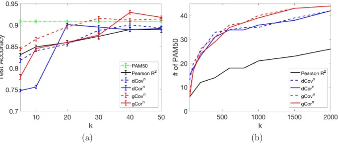
n is large, using a random subset of samples for dependence estimations is recommended. Since gGor measures the dependence between a numerical variable and a categorical variable, it is well suited to serve as a feature selector in a classification problem. One of our previous work (Zhang et al., 2019) is to use gCor or gCov to rank feature relevance and showed that gCor and gCov outperformed dCor, dCov and Pearson correlation. To apply Pearson correlation, we treated the class variable as numerical. To apply dCor or dCov, we used set difference to measure the sample distances of the class variable, i.e., the distance between to samples is 1 if they are of different classes, or 0 otherwise. Figure 2.1 shows the ranking performance of using Pearson R2, dCov, dCor, gCov and gCor. PAM50 is the gold standard gene list for breast cancer subtype diagnosis. In both subfigures, k is the number of top features being selected. Figure 2.1a shows that gCov and gCor are able to select a smaller set of genes and the prediction is better than the gold standard. Figure 2.1b shows that Gini statistics are able to select more PAM50 genes than distance statistics ask
(a) (b)
Figure 2.1. Feature selection on the breast cancer dataset. (a) Test accuracy using the top k selected genes. (b) Number of PAM50 genes in the selected topk genes.
increases.
2.4 Permutation Tests
Like other statistical tests, ap-value needs to be calculated to measure the significance of dependence. Thep-value is the probability of observing the test statistic or higher when the null hypothesis is true. A smaller p-value suggests the higher significance of the test. In our dependence test, if we use gCorn(X, Y) as the test statistic (similar if we use dCorn(X, Y)),
we will have the following null and alternative hypotheses:
H0 : gCor(X, Y) = 0,(X and Y are independent);
H1 : gCor(X, Y)>0,(X and Y are dependent).
A claim on dependence can be make by comparing thep-value with a pre-defined significance level α: if p−value 6 α, we reject the null hypothesis and claim X and Y are dependent. For example, if we we observe gCorn(X, Y) = 0.01 in our dependence test, ap-value = 0.045 is interpreted as: when X and Y are independent, P(gCorn(X, Y) > 0.01) = 0.045. If the significance level α is set at 0.05, we can reject the null hypothesis and say X and Y are
dependent. The p-value is crucial for two reasons: 1) it can be used to determine whether or not two random variables are dependent; 2) thep-values of dependence tests can be used to sort the significance of dependence, e.g., in the application of feature selection.
A common approach to calculate p-value is to perform permutation tests. A per-mutation test is to calculated the test statistic (gCorn(X, Y) in the example above) after random permutating the sample observations of X or Y. After N permutation tests, the p-value can be estimated by the proportion of test statistics obtained in permutation tests that are greater than the observed test statistic in the dependence test, i.e.,
p−value =
PN
i=1I(gCorn(X, Y)ithperm >gCorn(X, Y))
N , (2.2)
where gCorn(X, Y)ithperm is the notation for gCorn(X, Y) obtained in the ith permutation test and I(·) is the indicator function. The larger the value of N is, the more accurate the p-value can be obtained. Therefore in our implementation, we used a relative large N (N = 5000) and parallelized permutation tests.
CHAPTER 3
FEATURE LOCALITY
3.1 Motivation
The idea of feature locality comes from the observation that convolutional neural networks (CNNs) are good at analyzing image data due to their ability to learn abstract representations from local features (pixels). In spite of their excellent performance, CNNs are black-box models that lack interpretability. This motivated us to borrow the idea of exploiting local information from CNNs to improve random forests, which are much more interpretable (discussed in Section 1.3).
Is local information of features useful to a random forest? The answer is yes, if the following hypothesis is true: features within a shorter distance are more dependent than features across a longer distance. For image data, the distance between features can be defined by the Euclidean distance between pixels on the 2D grid. For non-image data, the distance between features needs to be defined. We show some experimental results to validate our hypothesis below, but let’s assume the hypothesis is true for now. We can therefore increase the variance of the tree outputs by constructing the forest in this way: we use a subset of features (instead of all features) as the input for each tree and let local features be in the same tree. As a consequence, features input to different trees are less correlated. Since a tree classifier is just a function mapping from input to output, by making the inputs less correlated, we are also forcing the outputs from different trees to be less correlated. Mathematically, letAandB be two subsets of features, andXA,XB be the data represented using feature set A and B, respectively. We then train a tree TA using feature
generate TA and TB, respectively. Then the class conditional correlation between these two trees is ρ(ΘA,ΘB|Y) =ρX(rmg(ΘA,X, Y), rmg(ΘB,X, Y)) ∝CovX(rmg(ΘA,X, Y), rmg(ΘB,X, Y)) = CovX(rmg(ΘA,XA, Y), rmg(ΘB,XB, Y)) =EX[rmg(ΘA,XA, Y)rmg(ΘB,XB, Y)] −EXA[rmg(ΘA,XA, Y)]EXB[rmg(ΘB,XB, Y)] = Z rmg(ΘA,xA, Y)rmg(ΘB,xB, Y)p(xA,xB|Y)dx − Z rmg(ΘA,xA, Y)p(xA|Y)dxA Z rmg(ΘB,xB, Y)p(xB|Y)dxB = Z rmg(ΘA,xA, Y)rmg(ΘB,xB, Y)p(xA,xB|Y)dx − Z rmg(ΘA,xA, Y)rmg(ΘB,xB, Y)p(xA|Y)p(xB|Y)dx = Z rmg(ΘA,xA, Y)rmg(ΘB,xB, Y)[p(xA,xB|Y)−p(xA|Y)p(xB|Y)]dx 6{ Z [rmg(ΘA,xA, Y)rmg(ΘB,xB, Y)]2dx Z [p(xA,xB|Y)−p(xA|Y)p(xB|Y)]2dx}1/2. (3.1)
Notice that the second integral in ( 3.1) is a dependence measure ofXA andXB. By making
XA and XB less dependent, we can reduce the correlation between trees. In Chapter 1 we showed that the performance of random forest is controlled by the trade-off between strength and correlation. When the strength of individual trees is high enough, reducing the correlation is likely to improve the forest’s performance.
3.2 Feature Dependence in Image Data
To validate our hypothesis empirically, we need a way to measure the dependence between features. Specifically, we are more interested in measuring dependence between two
groups of features, and the sizes of the two groups are not necessarily to be the same. The two groups of features can be viewed as two random vectors, possibly of different dimensions. An observation of the random vector is a sample represented by the features of that group. Therefore, measuring the dependence between the two groups of features is equivalent to measuring the dependence between the two random vectors. As introduced in Section 2.2, distance correlation (dCor) is a good dependence measure for random vectors of arbitrary and not necessarily equal dimensions. It is zero if and only if the two random vectors are independent.
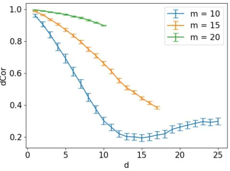
We tested our hypothesis on one of the most popular image data sets: MNIST (LeCun et al., 2010). In our experiment, we randomly selected twom bymwindows from the image as the two feature sets and tested the distance correlation of the two sets. 500 random samples (images) were used to calculate distance correlation. For implementation simplicity, the two windows under dependence test were of the same size, but they were not required to be. The window distance is measured by the Euclidean distance between the two left corner pixels of the two windows on the image and rounded to an integer. Given two pixelsp1 and
p2 with their coordinates on the image being (x1, y1) and (x2, y2), the distance between p1 and p2 is defined as
d=p(x1 −x2)2+ (y1−y2)2. (3.2)
A schematic diagram of our experiment is shown in Figure 3.1. The conditional distance correlation dCor(X1,X2|Y) was first calculated and the unconditional distance correla-tion is calculated by taking the expectacorrela-tion of the dCor(X1,X2|Y), i.e., dCor(X1,X2) =
EY[dCor(X1,X2|Y)]. Here X1 and X2 denotes the two sets of features defined by the two windows andY denotes the class label. The results are shown in Figure 3.2. Three different values of window size m were used: 10, 15 and 20. The range of the window distance is defined by the window size since the images are of a fixed size of 28 by 28. The distance was rounded to an integer for plotting and each point in the figure is an average of 100 experi-ments. The figure shows a clear trend of decreasing dependence when the distance between
Figure 3.1. A schematic diagram of testing dependence between two windows of size m×m on MNIST data. The distance between two widows d is measured by the distance between the upper left corners of the windows.
the two windows is increased, which validates our hypothesis empirically. For window size m = 10 with d > 15, the slightly increase in dCor is because both windows include some margins of the image (black background regions).
3.3 Local Features of Non-Image Data
For non-image data, feature locality is not explicitly given as in the case of images, therefore it has to be defined or learned from the data. To learn the neighborhood infor-mation of the features, the pair-wise distance needs to be defined. The goal of defining the distance is to capture feature dependence such that dependent features should have a closer distance to each other. Therefore it is appealing to use a dependence measure to repre-sent the distance. As discussed in Section 2.2, dCor is a good candidate for this purpose, but the computation is too expensive for pair-wise feature dependence measures, which is (O(n2d2)), where d is the number of features). To reduce computation complexity, we use Pearson correlation as a substitute. Other distance metrics that have been used in data visualization and dimensionality reduction techniques are also worth testing, since they are good approximations for sample dependence. Here we propose four ways of defining the pair-wise distance between features. Each feature can be represented by its values in the samples, i.e., a vector of length n, where nis the number of samples. The following distance
Figure 3.2. Feature dependence tested using distance correlation statistic on MNIST dataset.
metrics are used in our study to calculate pair-wise distance of features: 1) 1−ρ2, where ρ is the Pearson correlation; 2) Euclidean distance; 3) PCA Euclidean and 4) graph distance. The first one is a direct approach to capture feature dependence. Euclidean distance is the most commonly used distance metric in data analysis. PCA Euclidean is defined as the Euclidean distance between features after dimensionality reduction using PCA (Principle Component Analysis). This is the default distance used int-SNE implementation in Python scikit-learn. The graph distance is defined as the shortest path between two features in the k-neighbor graph. In the k-neighbor graph, each node is a feature and it has undirected edges to its k-nearest neighbors defined by Euclidean distance and the weight of the edges are the Euclidean distances. This distance is used in the Isomap algorithm for dimension-ality reduction (Tenenbaum et al., 2000) and is good for the Swiss Roll dataset. However, the choice of k is tricky and the graph can also be defined as a unweighted graph, which makes it difficult to find the optimal and stable distance representation for different datasets. We show the evaluation of the above mentioned distance metrics in Chapter 4. Once the pair-wise distance of features is defined, a random set of “local” features of size m can be
selected by randomly choosing a feature and its (m−1) nearest neighbors.
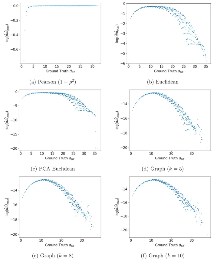
To provide some insight on how well these distances are defined, we compute these distances, denoted as ˆd, using the MNIST data and compare those with the ground truth, dGT, which can be obtained by (3.2). For each distance type we defined, a scatter plot
is generated and shown in Figure 3.3. The x-axis is the ground truth, the y-axis is the logarithmic of the normalized distance learned from the data. Since a particular value of dGT may correspond to multiple values of ˆd, the median of which is used to generate the
plot. A perfect distance measure should have a monotonic increasing trend asdGT increases.
As shown in Figure 3.3, none of the distance defined maintains monotonic increasing trend in the whole x-range. All of them serve as a good distance measure only within a certain range. Pearson distance is functional only when dGT is less than 5. log( ˆd/dˆmax) is close to 0
when dGT >5. This is because a pair of pixels with a distance longer than 5 in between on
the images has a Pearson correlation close to 0, resulting ˆdto be near 1. Euclidean and PCA Euclidean are functional when dGT <7. Graph distances have a longer functional range, up
to dGT = 12. The behavior is not sensitive to the different choices of k. From the above
results, Graph distances seem like better distance measures when the ground truth is not available.
3.4 Summary
In this Chapter, we presented the concept of feature locality. For image data, the locations of features are given by their coordinates on the image. We validated that pixels within a shorter distance have higher dependency. For non-image data, we aim to find a organization of the features such that dependent features are clustered together. To achieve this goal, since the direct measure of dependence between every pair of features by distance correlation is too computationally expensive, we presented alternative ways of defining dis-tance that captures dependence. The proposed disdis-tance measures were tested on the MNIST dataset and compared with the ground truth (distance defined by the pixel coordinates). The
(a) Pearson (1−ρ2) (b) Euclidean
(c) PCA Euclidean (d) Graph (k = 5)
(e) Graph (k= 8) (f) Graph (k = 10)
graph distances show more promising results than others. In the next chapter, we show how to utilize feature locality to improve random forests.
CHAPTER 4
RANDOM FOREST WITH LOCAL FEATURE SAMPLING
4.1 Local Feature Sampling
The most popular way of building a random forest is by training each tree with boot-strap samples using all features. It has also been proposed to use a random subset of features to grow each tree, know as “the random subspace” (Barandiaran, 1998). However, the fea-tures in the subset are chosen by a pure random sampling without considering any locality information of the features. Here we propose alocal feature sampling (LFS) approach, which is also using a feature subspace but our contribution is to include the locality information during the sampling process, i.e., a random patch or neighbourhood of features are used to construct each tree. In (Louppe, 2014), the term “random patch” is also used but what it actually means is random subspace. We name our version of random forest as RF-LFS (random forest with local feature sampling).
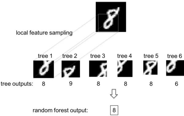
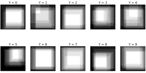
For image data, a random patch is defined by an m × m square region of pixels (totalm2 features) located at a random position in the image. The sampling process can be achieved by randomly picking a pixel from the image as the upper left corner of the patch and including all features in the m×m square. Notice that the valid region for picking the upper left corner pixel is not the whole image but a cropped image of size (M−m)×(M−m) if the whole image is of sizeM×M. An example of how RF-LFS works on predicting a digit ‘8’ is shown in Figure 4.1. The forest consists of 6 trees. Each tree has access to a random local region of the image during training and testing. This introduces varieties in the tree outputs since different trees have different access to the data. For example, tree 2 predicts ‘9’ because it looks at the top part of digit ‘8’ while tree 6 predicts ‘6’ since it looks at the
Figure 4.1. An example of how RF-LFS works on predicting a digit ‘8’.
bottom part. However, the majority votes for ‘8’ which is correct.
For non-image data, a random neighbourhood of size m is generated by randomly selecting one feature from the whole feature set and then its (m−1) nearest neighbours with the distance defined using one of the distance metrics described in Section 3.3. Therefore, a pair-wise distance metric of features needs to be calculated before the construction of trees.
4.2 Sampling Window Size
We call the size of a random patch or neighbourhood as the sampling window size. When the sampling window size is equal to the total number of features, then LFS is equiva-lent to not using LFS. Therefore, the default setting of current random forest can be viewed as a special case of our RF-LFS. The window size among trees can be kept the same or using a random size for each tree. In the former case, the window size is a hyper-parameter and in the latter case, the range of the window size is a hyper-parameter. We compare these two cases in Section 4.4.1.
4.3 Out-of-Bag Estimates of Error, Strength and Correlation
We implemented out-of-bag estimates of error, strength and correlation in the RF-LFS classifier, as described in Section 1.5. The estimates of strength and correlation help us in understanding how LFS affects the model and the out-of-bag error can be used as the validation performance to optimize hyper-parameters. Notice that the out-of-bag estimates require bootstrap. Since bootstrap is usually recommended to train random forests, we use bootstrap for all experiments.
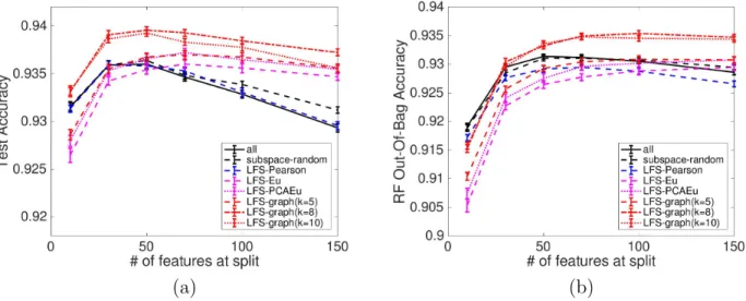
4.4 Experimental Results 4.4.1 The MNIST Dataset
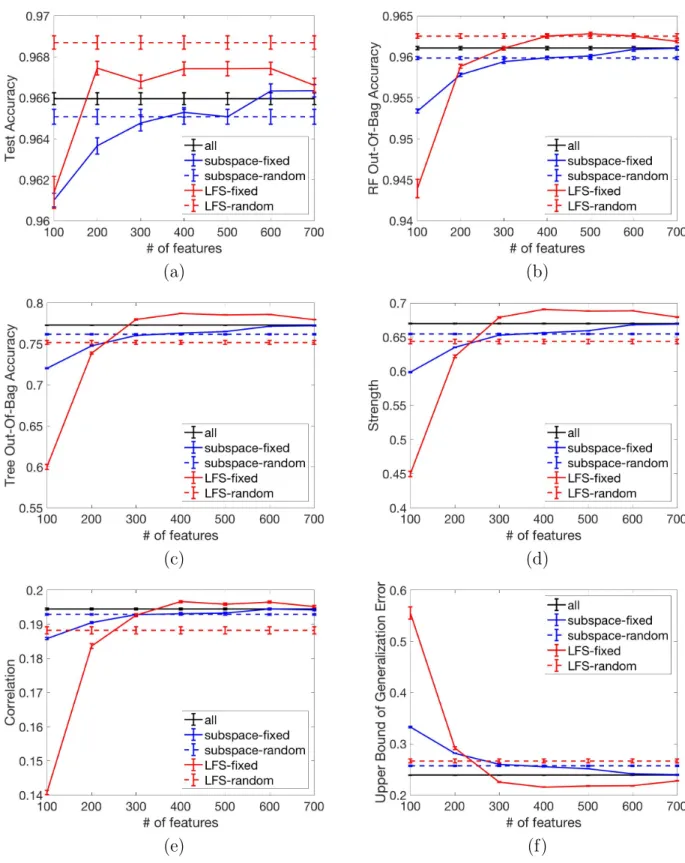
We first tested RF-LFS on the most popular benchmark image dataset, the MNIST dataset. We compare RF-LFS with 1) fixed and 2) random window size against the other three non-LFS based RFs as baselines: 3) RF using all features (this is the Python scikit-learn implementation); 4) RF using random subspaces with fixed size and 5) RF using random subspaces with random sizes. We use the following legends for the five methods under comparison: 1) LFS-fixed; 2) LFS-random; 3) all; 4) fixed and 5) subspace-random.
Figure 4.2 shows the results of test accuracy, RF out-of-bag accuracy (performance of RF on out-of-bag examples), tree out-of-bag accuracy (average performance of trees on out-of-bag examples), strength (out-of-bag estimates), correlation (out-of-bag estimates) and upper bound of generalization error (Theorem 1). The number of features sampled to grow each tree is a hyperparameter for subspace-fixed and LFS-fixed, but not for the other three methods. Therefore, we show the effect of this hyperparameter on the performance by using different values from 100 to 700. Each data point in the curve is the average of 30 runs. For method all, subspace-random, and LFS-random, a straight line is plotted. Among all five methods under comparison, LFS-random has the best performance (test accuracy), regardless of the hyperparameter used for other methods.
(a) (b)
(c) (d)
(e) (f)
Table 4.1. Performance on the MNSIST Dataset Using Optimal Number of Features for Sampling.
Method Validation (%) Test (%) Strength Correlation
all 96.11 96.60 0.670 0.195
subspace-fixed 96.09 96.63 0.668 0.195
subspace-random 95.98 96.51 0.655 0.193
LFS-fixed 96.25 96.74 0.691 0.197
LFS-random 96.25 96.87 0.644 0.188
We use RF out-of-bag accuracy as validation accuracy to choose the optimal number of features used for sampling and compare test accuracy. The results are shown in Table 4.1. The performance gain of LFS-random is due to the reduced correlation with sacrifice in strength. The decrease in strength is because of the use of local features, as expected. How-ever, since now the correlation is more dominant in controlling the overall forest performance, reducing correlation among trees is beneficial. The fact subspace-fixed and LFS-random out-performs subspace-random shows that the performance gain comes from the local features sampling, rather than a simply usage of random subsets of features.
From Figure 4.2(f), we can see that the upper bound is loose, therefore does not correspond with test accuracy. This suggests that a lower upper bound on generalization error does not guarantee a higher test accuracy. Therefore it is more reasonable to use RF out-of-bag accuracy to optimize hyperparamters. Figure 4.2(d)&(c) also show the trade-off between strength and correlation, i.e., one cannot increase strength as well as reduce cor-relation at the same time. Since LFS-random outperforms LSF-fixed and subspace-random is comparable with subspace-fixed, we omitted methods with fixed sampling size for later experiments and no optimization on sampling size is further needed.
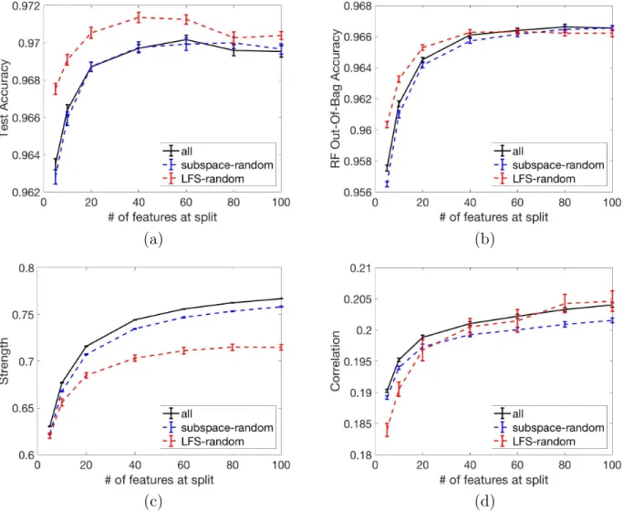
Notice that using LFS is not the only way to control the trade-off between strength and correlation, other hyperparameters like bootstrap and number of features used at each split (the max features parameter of sklearn.ensemble.RandomForestClassifier) are also key hyperparameters that achieve this goal. The results shown in Figure 4.2 were obtained by setting bootstrap as true and number of features at each split as log2(n f eatures). Our
(a) (b)
(c) (d)
Figure 4.3. The MNIST dataset. Effect of number of features at each tree node to decide best split.
LFS is a third hyperparameter that should be tested along with these two to see if a third one is helpful. We keep bootstrap on for all tests and we compare LFS-random against all and subspace-random by varying the value for number of samples at split. The effect of the number of features at each split on the performance is shown in Figure 4.3. The performance gain due to LFS is small but significant. The validation and test accuracies, strength and correlation using the optimal number of features at each split are shown in Table 4.2.
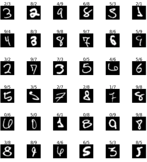
We randomly selected 100 images from the test set that RF-all predicted wrong but RF-LFS-random predicted correctly, as shown in Figure 4.4. These are examples showing local information is more critical and generalizable than global information. For example,
Table 4.2. Performance on the MNIST Dataset Using Optimal Number of Features at Each Split.
Method Validation (%) Test (%) Strength Correlation
all 96.66 96.96 0.763 0.203
subspace-random 96.66 96.97 0.758 0.202
LFS-random 96.63 97.14 0.703 0.201
the image on the second row, second column is a “3”, but it is so thick that RF-all predicted it as an “8”. The image on the 5th row, 5th column is a “9”, but RF-all interpreted it as a “0” because there is a big circle. However, by using local features, LFS was able to predict these images correctly.
We are also interested in what regions (groups of features) are essential to make the prediction correct for each class. Therefore, for each class, we selected the 10 trees in the forest that have highest accuracy for this particular class, and visualize the patches they used. The visualization result is shown in Figure 4.5. The white pixels are features selected and the intensity shows the frequency of a pixel being selected. It shows that trees have different focuses for different classes.
4.4.2 The ISOLET Dataset
We next test LFS on a non-image dataset—the ISOLET dataset, available at UCI Machine Learning Repository (Dheeru and Karra Taniskidou, 2017). This dataset contains recordings of human speaking letters from “a” to “z”. The number of classes is 26, the number of examples is 7797 and the number of features is 617. We randomly hold out 50% of the data as test set and the other 50% as training set.
Since this is a non-image dataset, we need to choose a distance metric to define feature neighborhood. As mentioned in Section 3.3, we will test Pearson, Euclidean, PCA Euclidean and graph distance. Specifically, for the graph distance, the value of k needs to be determined to construct the k-neighbor graph. Here we tested the value of k to be 5, 8 and 10. The legend for methods under comparison are:
Figure 4.4. Some example images that RF-all predicted wrong but RF-LFS-random predicts correctly. The prediction result is shown in the format of “all/LFS” on the top of each image.
Figure 4.5. Random patches used by top-10 trees with highest accuracy for each class.
• all: RF using all features;
• subspace-random: RF using a random subset (of random size) of features without considering feature locality;
• LFS-Pearson: RF with LFS with random window size using (1−ρ2) as the distance to define feature neighborhood;
• LFS-Eu: RF with LFS with random window size using Euclidean distance to define feature neighborhood;
• LFS-PCAEu: RF with LFS with random window size using Euclidean distance of features after dimensionality reduction using PCA. The number of components used for this dataset is 20;
• LFS-graph (k = n): RF with LFS with random window size using shortest path on the k-neighbor graph as the distance, wherek =n.
The performance of methods under evaluation are shown in Figure 4.6. Each data point is an average of 100 runs. It is obvious that LFS-graph (k = 8) has the best performance in
(a) (b)
Figure 4.6. The ISOLET dataset. Effect of number of features at each tree node to decide best split.
Table 4.3. Performance on ISOLET Dataset Using Optimal Number of Features at Each Split.
Method Validation (%) Test (%) Strength Correlation
all 93.14 93.60 0.570 0.210 subspace-random 93.10 93.64 0.565 0.208 LFS-Pearson 92.92 93.58 0.534 0.188 LFS-Eu 92.88 93.56 0.486 0.175 LFS-PCAEu 93.08 93.55 0.501 0.181 LFS-graph (k = 5) 93.09 93.68 0.490 0.171 LFS-graph (k = 8) 93.49 93.93 0.487 0.165 LFS-graph (k = 10) 93.47 93.83 0.501 0.170
all x-range. The performances using optimal number of features at each split are shown in Table 4.3. As the table shows, all LFS methods based on graph distance outperform the sklearn implementation and subspace-random. It is also clear that the performance gain of these graph distance based LFS methods come from the reduced correlation. Among all distance metrics being tested, graph distance with k = 8 perform best and has the lowest correlation on this dataset. However, the optimalk can be data dependent. We chose to use graph distance with k set to 8 by default, as our distance metric for LFS to test on other non-image data.