Search-based Software Test Data Generation:
A Survey
Phil McMinn
The Department of Computer Science, University of Sheffield
Regent Court, 211 Portobello Street
Sheffield, S1 4DP,UK
This is a preprint of an article published in
Software Testing, Verification and Reliability,
14(2), pp. 105-156, June 2004.
Copyright (c) Wiley 2004.
Abstract
The use of metaheuristic search techniques for the automatic genera-tion of test data has been a burgeoning interest for many researchers in recent years. Previous attempts to automate the test generation process have been limited, having been constrained by the size and complexity of software, and the basic fact that in general, test data generation is an un-decidable problem. Metaheuristic search techniques offer much promise in regard to these problems. Metaheuristic search techniques are high-level frameworks, which utilise heuristics to seek solutions for combinato-rial problems at a reasonable computational cost. To date, metaheuristic search techniques have been applied to automate test data generation for structural and functional testing; the testing of grey-box properties, for example safety constraints; and also non-functional properties, such as worst-case execution time. This paper surveys some of the work under-taken in this field, discussing possible new future directions of research for each of its different individual areas.
Keywords: search-based software engineering; automated software test data generation; evolutionary testing; metaheuristic search; evolutionary algorithms; simulated annealing
1
Introduction
The use of metaheuristic search techniques for the automatic generation of test data has been a burgeoning interest for many researchers in recent years. In industry, test data selection is generally a manual process - the responsibility for which usually falls on the tester. However this practice is extremely costly, difficult and laborious. Automation in this area has been limited. Exhaustive
enumeration of a program’s input is infeasible for any reasonably-sized program, yet random methods are unreliable and unlikely to exercise “deeper” features of software that are not exercised by mere chance. Previous efforts have been limited by the size and complexity of the software involved, and the basic fact that in general, test data generation is an undecidable problem.
The application of metaheuristic search techniques to test data generation is a possibility which offers much promise for these problems. Metaheuristic search techniques are high-level frameworks which utilise heuristics in order to find solutions to combinatorial problems at a reasonable computational cost. Such a problem may have been classified as NP-complete or NP-hard, or be a problem for which a polynomial time algorithm is known to exist but is not prac-tical. They are not standalone algorithms in themselves, but rather strategies ready for adaption to specific problems. For test data generation, this involves the transformation of test criteria to objective functions. Objective functions compare and contrast solutions of the search with respect to the overall search goal. Using this information, the search is directed into potentially promising areas of the search space.
Search-based software test data generation is just one example of search-based software engineering [1, 2]. To date, metaheuristic search techniques have been applied to automate test data generation in the following areas:
• the coverage of specific program structures, as part of a structural, or white-box testing strategy;
• the exercising of some specific program feature, as described by a specifi-cation;
• attempting to automatically disprove certain grey-box properties regard-ing the operation of a piece of software, for example tryregard-ing to stimulate error conditions, or falsify assertions relating to the software’s safety;
• to verify non-functional properties, for example the worst-case execution time of a segment of code.
This paper surveys work undertaken in these areas and the results achieved. Section 2 begins by reviewing some of the search techniques used. Section 3 discusses their application to structural testing, which to date has received the greatest share of attention from search-based testing researchers. Section 4 presents work in the area of functional testing, followed by grey-box testing (Section 5) and finally non-functional testing (Section 6). At the end of each section, the paper outlines possible directions for future research appropriate to that area.
2
Metaheuristic Search Techniques
In order to adapt a metaheuristic search technique to a specific problem, a number of different decisions have to be made - for example the way in which solutions should be encoded so that they can be manipulated by the search. A good choice of encoding will ensure that similar solutions in unencoded space are also “neighbours” in representational space. In this way, the search will be allowed to move easily from one solution to another that shares a similar
set of properties. These movements are dependent on the evaluation of can-didate solutions, performed using a problem-specific objective function. With feedback from the objective function, the search seeks “better” solutions based on knowledge and experience of previous candidates. A good objective function is therefore critical to the success of the search. Solutions that are “better” in some respect should be rewarded with better objective values, whereas poorer solutions should be punished with poorer objective values. Whether a “better” objective value is, in practice, a higher value or lower value, is dependent on whether the search is seeking to minimise or maximise the objective function. An objective function which is being maximised reflects the relative “goodness” of candidate solutions, whereas an objective function to be minimised (more usually referred to in this context as acost function) reflects the relative unde-sirability of solutions.
The next section outlines some metaheuristic techniques that have been used in software test data generation, namely Hill Climbing, Simulated Annealing and Evolutionary Algorithms. Further treatment of these search techniques can be found in reference [3]. The last decade has seen the emergence of many new techniques, which have not been exploited by the test data generation techniques presented here. Reference [4] gives treatment to some of these.
2.1
Hill Climbing
“Hill Climbing” is a well known local search algorithm. Hill Climbing works to improve one solution, with an initial solution randomly chosen from the search space as a starting point. The neighbourhood of this solution is investigated. If a better solution is found, then this replaces the current solution. The neigh-bourhood of the new solution is then investigated. If a better solution is found, the current solution is replaced again, and so on, until no improved neighbours can be found for the current solution.
This progressional improvement is likened to the climbing of hills in the “landscape” of a maximising objective function. In this landscape, peaks char-acterise solutions with locally optimal objective values, and troughs signify solu-tions with the locally poorest objective values. In a “steepest ascent” climbing strategy, all neighbours are evaluated, with the neighbour offering the great-est improvement chosen to replace the current solution. In a “random ascent” strategy (sometimes referred to as “first ascent”), neighbours are examined at random and the first neighbour to offer an improvement is chosen. A high level description of the algorithm can be seen in Figure 1.
Hill climbing is simple and gives fast results. However it is easy for the search to yield sub-optimal results when the hill climbed leads to a solution that is locally optimal, but not globally optimal. In such cases, the search becomes trapped at the peak of a hill, unable to explore other areas of the search space. The search will also become stuck along plateaux in the landscape. In such circumstances, no neighbouring solution is deemed to offer an improvement over the current solution, since they all have the same objective value. Therefore, in non-trivial landscapes, results obtained with hill climbing are highly dependent on the starting solution. A common extension to this algorithm is to incorporate a series of “restarts” involving different initial solutions, to sample more of the search space and minimise this problem as much as possible.
Select a starting solutions∈S
Repeat
Selects0∈N(s) such thatobj(s0)> obj(s) according to ascent strategy
s←s0
Untilobj(s)≥obj(s0),∀s0∈N(s)
Figure 1: High level description of a hill climbing algorithm, for a problem with solution space S; neighbourhood structure N; andobj, the objective function to be maximised
2.2
Simulated Annealing
It is desirable to have a search framework that is less dependent on the starting solution. Simulated Annealing is similar in principle to Hill Climbing. However, by probabilistically accepting poorer solutions, Simulated Annealing allows for less restricted movement around the search space. The probability of acceptance
pof an inferior solution changes as the search progresses, and is calculated as:
p=e−δt
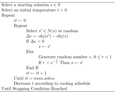
whereδis the difference in objective value between the current solution and the neighbouring inferior solution being considered, and t is a control parameter known as the temperature. The temperature is cooled according to a cooling schedule. Initially the temperature is high, in order to allow free movement around the search space, and so that dependency on the starting solution is lost. As the search progresses, the temperature decreases. However, if cooling is too rapid, not enough of the search space will be explored, and the chances of the search becoming stuck in local optima are increased. The basic algorithm, for minimising an objective function, can be seen in Figure 2.
The name “Simulated Annealing” originates from the analogy of the tech-nique with the chemical process of annealing - the cooling of a material in a heat bath. If a solid material is heated past its melting point, and then cooled back into a solid state, the structural properties of the cooled solid depend on the rate of cooling. An algorithm proposed by Metropolis et al. [5] simulates the change in energy of the system when subjected to a cooling process, until it converges into a steady state. This algorithm was later proposed as the basis of the search mechanism by Kirkpatricket al. [6].
2.3
Evolutionary Algorithms
Evolutionary Algorithms use simulated evolution as a search strategy to evolve candidate solutions, using operators inspired by genetics and natural selection. Genetic Algorithms are probably the most well known form of Evolutionary Algorithm, having been conceived by John Holland in the United States during the late sixties. Genetic Algorithms are closely related to Evolution strategies, which were developed independently at the about the same time in Germany by Ingo Rechenburg and Hans-Paul Schwefel. For Genetic Algorithms, the search is primarily driven by the use of recombination - a mechanism of exchange of in-formation between solutions to “breed” new ones - whereas Evolution Strategies principally use mutation - a process of randomly modifying solutions. Although
Select a starting solutions∈S
Select an initial temperature t >0 Repeat it←0 Repeat Select s0∈N(s) at random ∆e←obj(s0)−obj(s) If ∆e <0 s←s0 Else
Generate random numberr, 0≤r <1 Ifr < e−δt Thens←s0
End If
it←it+ 1 Untilit=num solns
Decreasetaccording to cooling schedule Until Stopping Condition Reached
Figure 2: High level description of a Simulated Annealing algorithm, for a prob-lem with solution spaceS; neighbourhood structureN;num solns, the number of solutions to consider at each temperature levelt; andobj, the objective func-tion to be minimised
these different approaches were developed independently, and with different directions in mind, recent work has incorporated ideas from both traditions -narrowing the differences between the two. The discussion here, however, fo-cuses on Genetic Algorithms. For more information on Evolution Strategies, see references [7, 8, 9].
2.3.1 Genetic Algorithms
The name “Genetic Algorithm” comes from the analogy between the encoding of candidate solutions as a sequence of simple components, and the genetic struc-ture of a chromosome. Continuing with this analogy, solutions are often referred to as individuals or chromosomes. The components of the solution are some-times referred to as genes, with the possible values for each component called
alleles, and their position in the sequence the locus. Furthermore, the actual encoded structure of the solution for manipulation by the Genetic Algorithm is called the genotype, with the decoded structure known as the phenotype. For many applications, the genotype is simply a string of binary digits (this issue will be revisited in the context of test data generation). For example, a vector of three integers<112,255,52>in the range [0,255] might be represented as
<01110000,11111111,00110100>. For real values, a decision must made on the precision to be used and what mapping should be used to the binary strings. One possibility, for example, is to scale real values onto integer values according to the required precision, and then use an integer encoding.
Genetic Algorithms maintain a population of solutions rather than just one current solution. Therefore, the search is afforded many starting points, and the chance to sample more of the search space than local searches. The population
is iteratively recombined and mutated to evolve successive populations, known as generations.
The recombination operator takes two parent solutions and “breeds” them to produce two new offspring. In one-point recombination, a single crossover point is chosen at random. A recombination of two individuals<0,255,0>and
<255,0,255>,000000001111111100000000and111111110000000011111111
in encoded form, with a single-point crossover chosen to take place at locus 12, would take place as follows:
000000001111 111100000000
000000001111000011111111
111111110000 000011111111 111111110000111100000000
This produces two offspring -<0,240,255>and<255,15,0>.
Various selection mechanisms can be used to decide which individuals should be used to create offspring for the next generation. Key to this is the concept of the “fitness” of individuals. The fitness of an individual can be the value obtained directly from the objective function, or this value scaled in some way. The idea of selection is to favour the fitter individuals, in the hope of breeding fitter offspring. However, too strong a bias towards the best individuals will result in their dominance of future generations, thus reducing diversity and increasing the chance of premature convergence on one area of the search space. Conversely, too weak a strategy will result in too much exploration, and not enough evolution for the search to make substantial progress.
Holland’s original Genetic Algorithm [10] used fitness-proportionate selec-tion. In this selection mechanism, the expected number of times an individual is selected for reproduction is proportionate to the individual’s fitness in com-parison with the rest of the population. The process is analogous to the use of a roulette wheel. Each individual is allocated a slice of the wheel in proportion to its fitness. The wheel is then spunN times in order to pick N parents. At the end of each spin, the position of the wheel marker denotes an individual selected to be a parent for the next generation. Fitness-proportionate selec-tion has difficulties in maintaining a constantselective pressure throughout the search. Selective pressure is the probability of the best individual being se-lected, compared to the average probability of selection of all individuals. In the first few generations of the search, fitness variance is usually high. With fitness-proportionate selection, selective pressure will also be high, since the most highly-fit individuals will be granted the greatest opportunities to become parents. This can lead to premature convergence. Also in later generations, when fitness values amongst individuals are similar and the fitness variance of the population is correspondingly low, selective pressure is also low. This can lead to stagnation of the search.
Linear Ranking of individuals is a technique which proposes to circumvent this problem. Individuals are sorted by fitness, with selection performed ac-cording to rank, rather than through the direct use of fitness values. A linear ranking mechanism with bias Z, where 1 < Z ≤ 2, allocates a selective bias of Z to the top individual, a bias of 1.0 to the median individual, and 2−Z
to the bottom individual. With a constant bias applied throughout the search, selective pressure is more constant and controlled [11].
Tournament Selection[12] is a noisy but fast rank selection algorithm. The population does not need to be sorted into fitness order. Two individuals are
chosen at random from the population. A random number, 0< r≤1, is then chosen. If r is less than p(where pis the probability of the better individual being selected), the fitter of the two individuals ‘wins’ and is chosen to be a parent, otherwise the less fit individual is chosen. The competing individuals are returned to the population for further possible selection. This is repeatedN
times until the required number of parents have been selected. In all probability, every individual is sampled twice, with the best individual selected for repro-duction twice, the median individual once, with the worst individual remaining unselected. The resulting selective bias is dependent onp. Ifp= 1, then in all probability a ranking with a bias of 2.0 towards the best individual is produced. If 0.5< p≤1, then the bias is less than 2.0.
Once the set of parents has been selected, recombination can take place to form the next generation. Crossover is applied to individuals selected at random with a probabilitypc(referred to as thecrossover rateorcrossover probability).
If crossover takes place, the offspring are inserted into the new population. If crossover does not take place, the parents are simply copied into the new population. After recombination, a stage of mutation is employed, which is responsible for introducing or reintroducing genetic material into the search, in the interests of maintaining diversification. This is usually achieved by flipping bits of the binary strings at some low probability ratepm, which is usually less
than 0.01.
A high-level description of a Genetic Algorithm can be seen in Figure 3. The initial population is generated at random, orseeded with pre-set individu-als. The search is terminated when some stopping criterion has been met, for example when the number of generations has reached some pre-imposed limit.
2.3.2 Advanced Encodings and Operators
Traditionally chromosomes are represented as a string of binary digits. A prob-lem with standard binary encoding is the disparity that can occur between solutions that are close to each other in unencoded solution space, but are far apart in the encoded binary representation. For example in a standard binary encoding the integer 7 is represented as 0111, yet 8 is represented as 1000. Therefore, the crossover and mutation operators must change all four bits to move from one integer value to the neighbouring other. An alternative is the use of a Gray code. A Gray code is a binary representation where adjacent integers are also Hamming distance 1 neighbours in Hamming space. For exam-ple, inStandard Binary Reflected Gray Code,7is represented as0100, and8as
1100. Empirical evidence has shown that Gray codes are generally superior to standard binary encodings [13, 14].
Goldberg argues that binary representation decomposes the chromosome into the largest number of smallest possible building blocks in order for the recombination and mutation operators to work most effectively [15]. However, this is disputed by Antonisse [16], who advocates the use of more expressive alphabets. Davis [17] supports this view. For nine real-world applications us-ing Genetic Algorithms over a variety of problem domains, Davis found that real-valued representations always outperformed binary encodings (real-valued encodings are also the representational choice of Evolution Strategies [9]). Of course, the use of a real-valued encoding raises the question of how crossover and mutation should work. The crossover operator only requires an underlying
Randomly generate or seed initial populationP
Repeat
Evaluate fitness of each individual inP
Select parents fromP according to selection mechanism Recombine parents to form new offspring
Construct new populationP0 from parents and offspring
MutateP0
P ←P0
Until Stopping Condition Reached
Figure 3: High level description of a Genetic Algorithm
sequence representation, and as such can operate as for binary encodings. Pos-sibilities for the mutation operator include the replacement of a real number in the chromosome with a new, randomly generated number. More advanced mu-tation operators are based onreal number creep. These operators sweep across the chromosome, pushing values up and down by a small amount. In this way, an element of local search is incorporated [17].
Genetic Algorithms have been successfully applied to a wide range of prob-lems. For introductory texts, see references [15, 18]. For shorter overviews and tutorials, see references [19, 9, 20].
3
Structural (White-Box) Testing
Structural, or white-box testing is the process of deriving tests from the inter-nal structure of the software under test. This section summarises some of the achievements in automating structural test data generation through the use of metaheuristic techniques. These are compared with earlier related approaches. Before this, some basic concepts are reviewed.
3.1
Basic Concepts
Many forms of structural testing make reference to thecontrol flow graph(CFG) of the program in question. A control flow graph for a programF is a directed graphG= (N, E, s, e), whereN is a set of nodes,E is a set of edges, andsand
e are respective unique entry and exit nodes to the graph. Each node n∈ N
is a statement in the program, with each edge, e= (ni, nj)∈E, representing
a transfer of control from node ni to node nj. An example of a control flow
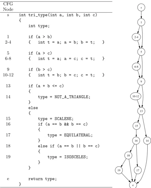
graph can be seen for a version of a triangle classification program in Figure 4. The triangle classification program is a benchmark used in many testing papers. Assuming three non-zero, non-negative integer lengths for the sides of a triangle, the program decides if the triangle is isosceles, scalene, equilateral, or invalid. Nodes corresponding to decision statements (for an example anifor a
whilestatement) are referred to as branching nodes. In the triangle example, branching nodes are nodes 1, 5, 9, 13, 16 and 18. Outgoing edges from these nodes are referred to asbranches. The condition determining whether a branch
is taken is referred to as thebranch predicate. For the true branch from node 1, the branch predicate isa > b.
An input vector I is a vectorI = (x1, x2, . . . , xk) of input variables to the
program F. The domain of an input variable xi, 1 ≤ i ≤ k, is the set if all
values thatxi can take on. Thedomain of the programF is the cross product D=Dx1×Dx2×. . .×Dxk where eachDxi is the domain for the input variable
xi. A program input x is a single point in the k-dimensional input space D,
x∈D.
A pathPthrough a control flow graph is a sequenceP =< n1, n2, . . . , nm>,
such that for all i,1≤i < m, (ni, ni+1) ∈E. A path is said to befeasible if there exists a program input for which the path is traversed, otherwise the path is said to be infeasible.
Adefinition of a variable vis a node which modifies the value ofv, for ex-ample an assignment statement or an input statement. The variable typeis defined in the triangle program at node 14. Ause of a variablev is a node in whichv is referenced, for example in an assignment statement, an output state-ment, or a branch predicate expression. In the triangle classification example, the variablesaandbare used at node 1.
Adefinition-clear path with respect to variablev is a path within which v
is not modified. In the triangle example, all paths from node 13 are definition-clear with respect to variables a, band c. However, no path from node 13 is definition clear with respect totype.
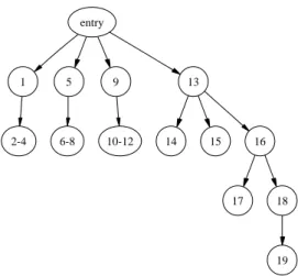
The term control dependency is used to describe the reliance of a node’s execution on the outcome at previous branching nodes [21]. A node z is post-dominated by a node y in Gif and only if every path from y to the exit node
e containsz. Node z post-dominates a branch (y, x) if and only if every path from y to the exit node e through (y, x) contains z. The node z is control dependent ony if and only ifzpost-dominates one of the branches of y, and z
does not post-dominatey. In the triangle example, node 17 is control dependent on node 16, which in turn is control dependent on node 13. Node 13 itself has no control dependencies, other than that of the external condition, entry, that causes the procedure to be executed. This information can be captured by a control dependence graph. Figure 5 shows the control dependence graph for the triangle program.
The techniques now described have been implemented for experimentation with a variety of programming languages. For consistency, however, all examples here are presented in C.
3.2
Static Structural Test Data Generation
Static structural test data generation is based on analysis of the internal struc-ture of the program, without requiring that the program is actually executed.
3.2.1 Symbolic Execution
Symbolic Execution [22, 23] is not the execution of a program in its true sense, but rather the process of assigning expressions to program variables as a path is followed through the code structure. The technique can be used to derive a
CFG s 1 2-4 5 6-8 9 10-12 13 15 14 16 18 17 19 e Node
s int tri_type(int a, int b, int c)
{ int type; 1 if (a > b) 2-4 { int t = a; a = b; b = t; } 5 if (a > c) 6-8 { int t = a; a = c; c = t; } 9 if (b > c) 10-12 { int t = b; b = c; c = t; } 13 if (a + b <= c) { 14 type = NOT_A_TRIANGLE; } else { 15 type = SCALENE; 16 if (a == b && b == c) { 17 type = EQUILATERAL; } 18 else if (a == b || b == c) { 19 type = ISOSCELES; } } e return type; }
Figure 4: A triangle classification program and its corresponding control flow graph
entry
1 5 9 13
2-4 6-8 10-12 14 15 16
17 18
19
Figure 5: Control dependence graph for the triangle classification program from Figure 4
constraint system in terms of the input variables which describes the conditions necessary for the traversal of a given path [24, 25, 26].
A forward traversal (or forward substitution) of a path, can be demonstrated with the triangle classification program in Figure 4. Say the path< s,1,5,9,10,
11,12,13,14, e >is to be executed. The input variablesa,bandcare assigned the constant variablesi,jandkrespectively. At nodes 1 and 5, the respective false branches are to be taken. Therefore, the first and second constraints of the constraint system for this path are:
(1)i <= j
(2)i <= k
The path also requires that the true branch be taken from node 9. This requires the addition of a third constraint:
(3)j > k
The following expressions are assigned at nodes 10 through to 12 respectively:
t = j b = k c = t
A fourth and final constraint from node 13 then needs to be added. Witha = i,
bnow equal tok, andc = t = j, this becomes: (4)i + k <= j
Backward path traversal is also possible, starting with the final node and following the path in a reverse manner to the start node. The resulting con-straint system is the same as for forward traversal, but no storage is required for the intermediate symbolic expressions of variables. Forward traversal, how-ever, allows for early detection of infeasible paths if the constraints generated
are inconsistent. Consider the path < s,1,2,3,4,5,6,7,8,9,13, . . . , e > which requires that the true branches are taken from nodes 1 and 5, and that the false branch from node 9 is taken. The constraints derived from the branching predicates from the initial section of the path through to node 9 are:
(1) i > j
(2) j > k
(3) i <= j
Clearly constraints 1 and 3 are contradictory, indicating that the path is in-feasible. Backward traversal would have meant symbolic execution of the path backwards fromethrough to 13 first, and then backwards through the nodes to node 1 before it would be possible to determine this fact.
Solutions to the constraint system are input data which will execute the path. Constraint satisfaction problems are in general NP-complete [27]. How-ever, if the constraints are linear, linear programming techniques can be applied [24]. Heuristic methods can be used in to attempt the finding of a solution where this is not the case. For example Boyeret al. [25] employ Hill Climbing. Ramamoorthyet al. [26] use a trial and error procedure, monitoring the effects of random-value assignments to variables in the constraint system. It is unlikely, however, that this procedure would be efficient for non-trivial programs.
If the test goal is the execution of a particular statement, all paths leading to the statement are explored. This is a problem in the presence of loops, due the potential number of paths that may need to be examined. In Clarke’s test data generator system [24], a path has to be manually selected by the tester. Many generators symbolically simply execute the loopKtimes, whereKis specified by the tester or chosen by the system [26]. A large number of constraints generated using this method, however, are not satisfiable.
Symbolic execution has several other problems, for example resolving com-puted storage locations such as array subscripts.
a[i] = 0; a[j] = 1; if (a[i] > 0) {
// perform some action }
In the above code fragment, it is not known in general whether a[i]anda[j]
refer to the same element, because the variablesiandjare not bound to specific values. This information is important, since ifiandjare equal, then the value of a[i] in the condition is 1 and the branch predicate evaluates to true. If not, the value of a[i] is 0 and the predicate evaluates to false. Boyer et al.
[25] and Ramamoorthy et al. [26] suggest possible solutions to this problem. Both methods significantly increasing the complexity and memory requirements of the Symbolic Execution system. A similar problem occurs with the use of pointers. In the following example, it is not known ifaandbrefer to the same location. Without this knowledge, the expression to assign to c can not be determined.
*a = 0; *b = 1; c = *a;
Further difficulties include the handling of procedure calls. A common solu-tion is to simply inline the called procedure into the calling routine [26]. However the number of paths can grow very rapidly with this approach.
Although any computable function can be written without the use of arrays, pointers or procedure calls, it is not normal practice for programmers to avoid such constructs simply because of the flexibility they offer, and the role they play in reducing the complexity of program code.
3.2.2 Domain Reduction
Domain reduction is a test data generation technique that was originally em-ployed as part of Constraint-based Testing, developed by DeMillo and Offutt [28]. Constraint-based Testing builds up constraint systems which describe the given test goal. The solution to this constraint system brings about satisfaction of the goal. The original purpose of Constraint-based Testing was to gener-ate test data for mutation testing. Reachability constraints within the con-straint system describe conditions under which a particular statement will be reached. Necessity constraints describe the conditions under which a mutant will be killed. Symbolic execution is used to develop the constraints in terms of the input variables. Domain reduction is then used to attempt a solution to the constraints. This procedure begins with the domains of each input variable. These can be derived from type or specification information, or be supplied by the tester. The domains are then reduced using information in the constraints, beginning with those involving a relation operator, a variable and a constant, and constraints involving a relation operator and two variables. Remaining constraints are then simplified by back-substituting values. When no further simplification is possible, the input variable with the smallest remaining do-main is chosen, and a random value is assigned to it. The value of this variable is then back-substituted throughout the constraint system, in order to allow further reduction of the domains of remaining variables. If all variables can be assigned values in this manner, then the constraint system will have been satisfied; otherwise the variable assignment stage is repeated, in the hope of this time successfully selecting appropriate random numbers for the variables.
With Constraint-based Testing, constraints must be computed before they are analysed. Since these constraints are derived using Symbolic Execution, the method suffers from similar problems involving loops, procedure calls and computed storage locations. Dynamic Domain Reduction was introduced by Offutt et al. [29] with the intent of addressing some of these issues. Although called Dynamic Domain Reduction, the technique still has the characteristic that the program is not executed with real input values. As with standard Do-main Reduction, Dynamic DoDo-main Reduction starts with the doDo-mains of the input variables. However, in contrast to standard Domain Reduction, these domains are reduced “dynamically” during the Symbolic Execution stage, us-ing constraints composed from branch predicates encountered as the path is followed. If the branch predicate involves a variable comparison, the domains of the input variables responsible for the outcome at the decision are split at some arbitrary “split point”, rather than assigning random input values. For example if the initial domains of two input variables yandzare [-10...10] and a branch predicate y < z is encountered which needs to be executed as true, the domains might be split leaving the domain of y to be [-10...0] and z to be
[1...10]. A back tracking procedure can be used to correct any spurious split points if the execution can only proceed so far down the specified path, and is unable to continue further due to a bad decision made earlier in the reduction process.
Despite setting out to deal with problems traditionally encountered by tech-niques based on Symbolic Execution, Dynamic Domain Reduction still suffers with difficulties due to computed storage locations and loops. Furthermore, it is not clear how domain reduction techniques handle non-ordinal variable types, such as enumerations.
3.3
Dynamic Structural Test Data Generation
As has already been discussed, the relationship between input data and internal variables for structural test data generation is difficult to analyse statically in the presence of loops and computed storage locations. Dynamic methods execute the program in question with some input, and then simply observe the results via some form of program instrumentation. Since array subscripts and pointer values are known at run-time, many of the problems associated with Symbolic Execution can be circumvented.
3.3.1 Random Testing
Random Testing simply executes the program with random inputs and then observes the program structures executed. This technique works well for simple programs. However structures that are only executed with a low probability are often not covered. Consider the triangle classification example once more (Figure 4). The true branch from node 16 requires that the three input values fora,bandcare all equal. Such a branch is unlikely to be executed by chance. Even if the domain of integer values for each variable were limited to values between 1 and 100, the probability of all three variables being selected with the same value is 1 in 10,000. In such cases a more directed search technique is required to locate test data.
3.3.2 Applying Local Search
Miller and Spooner [30] were the first to combine the results of actual executions of the program with a search technique. Their method was originally designed for the generation of floating-point test data, however the principles are more widely applicable. The tester selects a path through the program, and then produces a straight-line version of it, containing only that path. Branching statements are then replaced with a “path constraint” of the form ci = 0; ci > 0; or ci ≥ 0; where ci is an estimate of how close the constraint is to
being satisfied. For example, a branch predicate of the forma == b might be rearranged into the path constraintabs(a−b) = 0. Take the triangle example and the execution of the path < s, 1,5, 9, 10, 11,12, 13, 14, e > again. The straight-line program with its respective path constraints would be re-arranged as follows:
int tri_type(int a, int b, int c) { int type; (c1= (b−a))>= 0 int t = a; a = b; b = t; (c2= (c−a))>= 0 (c3= (b−c))>0 (c4= (c−(a+b)))>= 0 type = NOT_A_TRIANGLE; }
Note that the value of c2, c3 and c4 are dependent on the computations betweenc1 andc2. However, this information is not required for the derivation of the path constraints, as it would be for the process of test data generation using Symbolic Execution.
Using these constraints, a functionf is constructed. The value off provides a real-valued estimate of how close all of the constraints are to being satisfied, being negative when one or more of the constraints remains unsatisfied, and positive when all of the constraints are satisfied. Input values of a, b and c
are then sought through the use of numerical maximisation techniques, which attempt to push the value off closer and closer to zero, in the hope of eventually making it positive.
Under normal conditions, execution of the complete path is not possible until branch predicates encountered along the path are evaluated in the required manner. However, in the straight-line version of the program, it is possible for run-time errors to occur which would not have been possible in the original program. In the following segment of code, if execution is allowed to proceed down the true branch with values ofiless than zero, or greater thansize, an error will be induced, because the array index used in the assignment statement will be out of bounds:
if (i >= 0 && i < size) {
a[i] = 0; }
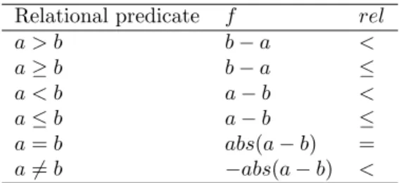
It was not until 1990 that the ideas of Miller and Spooner were extended by Korel [31] for Pascal programs. In this work, the test data generation procedure worked on an instrumented version of the original program without the need for a straight-line version to be produced. The search targeted the satisfaction of each branch predicate along the path in turn, circumventing issues encountered by the work of Miller and Spooner. To execute some desired path, the program is initially executed with some arbitrary input. If during execution an undesired branch is taken - one which deviates from the desired path - a local search for program inputs is invoked, using an objective function derived from the predicate of the desired, alternative branch. This objective function describes how “close” the predicate is to being true. The value obtained is referred to as thebranch distance.
Take the triangle example and the execution of the path < s, 1, 5, 9, 10,
11, 12, 13, 14, e > again. If the function is executed with the program input
Relational predicate f rel a > b b−a < a≥b b−a ≤ a < b a−b < a≤b a−b ≤ a=b abs(a−b) = a6=b −abs(a−b) <
Table 1: Korel’s objective functions for relational predicates
nodes 1 and 5. However control flow diverges away from the intended path down the false branch at node 9. At this point the local search is invoked to change the program inputs so that the alternative true branch is taken. If, in general, the branch predicate is assumed to be of the form a op b, where a
and b are arithmetic expressions and op is a relational operator, an objective function of the form f rel 0 is derived, wheref and relare given in Table 1. The function is to be minimised, being positive (or zero ifrelis ‘<’) when the current branch predicate for the required branch is false, and negative (or zero ifrel is ‘=’ or ‘≤’) when it is true. For the predicate of the true branch from node 9, the objective function isc - b > 0. The value of this function for the program input (a=10, b=20, c=30) is 30 - 20 = 10. The program must be instrumented so that objective values can be computed. This can be performed within the branching expression, for example as follows:
if (eval_obj(9, b, c)) {
...
Here, the program function eval_obj reports branch distances at node 9 using the local values ofbandc. This function will then return a boolean value corresponding to the evaluation of the original branching expression, in order for program execution to resume as normal.
The local search for deriving input values in accordance with the objective function is known as the alternating variable method. Each input variable is taken in turn and its value adjusted, keeping the other variable values constant. The first stage of manipulating an input variable is called theexploratory phase. This probes the neighbourhood of the variable by increasing and decreasing its original value. If either move leads to an improved objective value, a pattern
phase is entered. In the pattern phase, a larger move is made in the direction of the improvement. A series of similar moves is made until a minimum for the objective function is found for the variable. The next input variable is then selected for an exploratory phase.
Return to the triangle example again, for which execution had diverged from the intended path at node 9. Decreases and increases ofahave no effect on the objective value. Thereforebis chosen. A decrease ofbleads to a worse objective value, but an increase leads to an improvement. The pattern phase is entered for b, which will be increased until b > c. Suppose the value 31 is reached. The new input vector is now(a=10, b=31, c=30). Control flow now proceeds through branching node 9 as desired, however execution now diverges away at
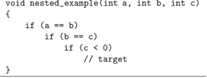
void nested_example(int a, int b, int c) { if (a == b) if (b == c) if (c < 0) // target }
Figure 6: Example with nested structures
node 13, since the value ofa + bat the node is greater than the value ofc. The local search is invoked again, this time to adjust the input values so that the true branch is taken from node 13, whilst maintaining the already correct sub-path up to this node. The new objective function, derived from the true branch predicate, is (a + b) - c <= 0. A decrease of the input value of bleads to a violation of the sub-path up to node 9, yet an improved value of the objective function is found for an increase of b (since the internal values of band care swapped at nodes 10-12). Eventually the input vector (a=10, b=40, c=30)
will be found. This input vector evaluates branching node 13 as true, and the complete path is executed.
As with all local searches, the final result is dependent on the starting so-lution. Consider the example of Figure 6. If the input is initially selected as
(a=10, b=10, c=10), control flow proceeds directly down to the final branch-ing node. However the variable c can not be changed to a value less than 0, because the already successful sub-path up to the final branching node will be violated. In this case, the search will fail.
Heuristic search methods have the potential to make moves through variable values that can not lead to an improvement in the value of the current cost function. This can lead to many wasteful and costly executions of the program. In the triangle example, changing the value of the input variable c does not have an effect on branching node 1. In order to make the search more efficient, Korel’s work makes use of extra information derived from the program, in the form of an “influences” graph. An influences graph is used to detect which input variables are able to influence the outcome at the current branching node, as determined using dynamic data flow analysis. A risk analysis of input variables is also undertaken in order to decide if they could potentially violate the already successful sub-path. For example at node 5, it is more attractive to manipulate
c rather than aor b, since changingaor b may change the current successful sub-path through node 1.
Gallagher and Narasimhan [32] built on Korel’s work for programs written in Ada. In particular, this was the first work to record support for the use of logical connectives within branch predicates. For predicates of the formA and B, the overall objective value is formed from the summation of the individual objective values of the expressions A andB. For predicates of the form A or B, the objective value is the minimum value of the individual objective values of the expressions.
3.3.3 The Goal-Oriented Approach
In his paper published in 1992, Korel developed what became known as the Goal-Oriented Approach [33]. All of the techniques concentrate on the execution of a path. For fulfilling a structural coverage criterion like statement coverage, this means a path has to be selected for each individual uncovered statement. The Goal-Oriented Approach removes this requirement. This is achieved through the classification of branches in the control flow graph of the program with respect to a target node as either critical, semi-critical or non-essential. This can be performed automatically on the basis of the program’s control flow graph.
For branches leaving a node on which the target is control dependent, a
critical branch is the edge which leads the execution path away from the target node. If control flow is driven down a critical branch, there is no prospect of the target being reached. Therefore, an objective function, of the form outlined in the previous section, is associated with the branch predicate of the alternative branch. The alternating variable search method is then employed to seek inputs so the alternative branch is taken instead. If the required inputs cannot be found, the overall process terminates, with the target remaining unexecuted.
A semi-critical branch is one which leads to the target node, but only via the backward edge of a loop. The alternative branch from the same branching node leads directly to the target node. In the case where the execution is driven down a semi-critical branch, the alternating variable method is again invoked to seek inputs for the execution of the alternative branch. If suitable input values cannot be found, however, the process does not terminate. Execution is allowed to flow down the semi-critical branch, in the hope of taking the alternative branch in the next iteration of the loop.
Finally, a non-essential branch is neither critical or semi-critical. Non-essential branches do not determine whether the target will be reached, regard-less of their position in the control flow graph. Therefore, execution is allowed to proceed unhindered through these branches.
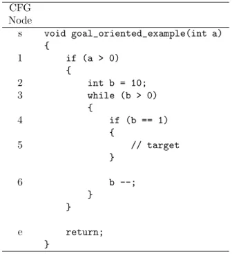
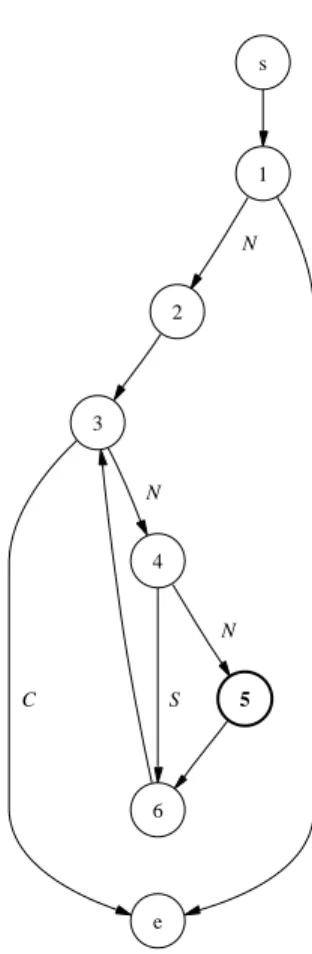
Take the example of Figure 7, with the target being the execution of node 5. The classification of each branch can be seen from the control flow graph in Figure 8. The false branches from nodes 1 and 3 are critical since node 5 cannot be reached if they are executed. The false branch from condition 4 is semi-critical, because although control flow diverges away from the target at this point, the target may still be reached in the next iteration of the loop. If the input vector is (a=0)the false branch from condition 1 is taken, and so the search procedure is invoked to change the value ofa. Control flow proceeds through down the true branch from node 1, but from node 4 the false branch is taken. However, the search can not change the outcome at this branch, and so the flow of control is allowed to continue around the loop a further nine times upon which the true branch from node 4 is taken, and the target is reached.
As the Goal-Oriented method also employs the alternating variable local search, it suffers from similar problems to those of Korel’s original approach. The removal of the requirement to select a path, although relieving some effort on behalf of the tester, introduces new ways in which the test data search can fail. Take the example of Figure 9 and the execution of the true branch from node 4. The true branch is only taken for objective values less than or equal to zero. Consider what happens when the initial input vector is selected so that a is less than zero (approximately half of the input domain). With such
CFG Node s void goal_oriented_example(int a) { 1 if (a > 0) { 2 int b = 10; 3 while (b > 0) { 4 if (b == 1) { 5 // target } 6 b --; } } e return; }
Figure 7: Example for the Goal-Oriented Approach
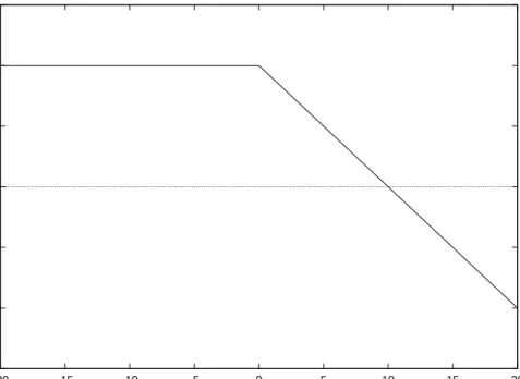
a starting point, the critical false branch from node 4 is taken. The search will fail, since small exploratory moves ofawill have no effect on the objective function associated with this condition, which is concerned only with the value ofb. The landscape of the objective function in this region of the search space is flat (Figure 10).
In this example, one could attribute the failure to the use of a local search technique. A global search technique such as a Genetic Algorithm is likely to sample the input domain more thoroughly and find the required value ofa. The local search could incorporate a series of restarts. However, it may be that the required path up to the target node is found with some very low probability. Even Genetic Algorithms will have trouble with these search spaces (see Section 3.5.4). Korel noted that this situation could be avoided if the data dependencies of the test goal were also taken into account by search, and attempted to address this issue with theChaining Approach.
3.3.4 The Chaining Approach
The Chaining Approach [34, 35] uses the concept of an event sequence as an intermediate means of deciding the type of path required for execution up to the target node. An event sequence is basically a succession of program nodes that are to be executed. The initial event sequence consists of just the start node and target node. Extra nodes are then inserted into this event sequence when the test data search encounters difficulties.
An event sequence can be formally described as a sequence of events < e1, e2,· · ·ek > where each event is a tuple ei = (ni, Ci) where ni ∈ N is a
s 1 2 N e C 3 4 N C 5 N 6 S
Figure 8: Control flow graph and branch classification for program in Figure 7. Node 5 is the target. C represents a critical branch;S, a semi-critical branch; andN, a non-essential branch
CFG Node s void chaining_approach_example(int a) { 1 int b = 0; 2 if (a > 0) { 3 b = a; } 4 if (b >= 10) { 5 // target } // ... }
Figure 9: Example for the Chaining Approach
-15 -10 -5 0 5 10 15 -20 -15 -10 -5 0 5 10 15 20
Objective Function Value
a
Figure 10: Objective function landscape for execution of node 4 as true for Figure 9
For every two adjacent eventsei= (ni, Ci) andei+1= (ni+1, Ci+1), no variables in the constraint set should be modified. That is to say a definition-clear path must be taken fromnito ni+1 with respect to each variable inCi.
For the example in Figure 9, the target is the execution of node 5. The initial event sequence is therefore:
<(s, φ),(5, φ)>
For every two adjacent eventsei = (ni, Ci) andei+1= (ni+1, Ci+1) in each event sequence E, the branches of the program are classed as either critical, semi-critical or non-essential. If there does not exist a definition-clear path with respect to the variables inCifromnitoni+1through branch (p, q), wherepand qare program nodes, yet such a path does exist from the alternate branch from
p, the branch (p, q) is declared critical. A branch (p, q) is semi-critical if it is not critical,ni+1is control dependent onp, and there does not exist an acyclic definition-clear path from pto ni+1 with respect toCi though (p, q). All other
branches are declared as non-essential. As with the Goal-Oriented approach, the flow of control should not take a critical branch. If one is taken, the alternating variable method is used to try and change the execution at the branching node. Semi-critical branches are preferably avoided, and non-essential branches are ignored.
Recall from the last section, the search for inputs to execute the branching node 4 as true for the program of program of Figure 9 can fail when the value of a is negative, e.g. -10. In executing the initial event sequence, the false branch from node 4 is critical. However, the local search is unable to find an input value ofa so that the alternative true branch is taken, since exploratory moves from-10yield no change in values of the objective function associated with this branch. When inputs can not be found to change the flow of control so that a critical branch (p, q) is avoided,pis “declared” as a problem node, for which new event sequences can be generated. In such instances the Chaining Approach looks for last definition statements of variables used at the problem node. In the example, the variable used at node 4 is the variable b. This variable is defined at nodes 1 and 3. Therefore, two different event sequences are generated, one inserting an event where node 1 should be executed and one where node 3 should be executed, i.e.:
1) <(s, φ),(1,{b}),(4, φ),(5, φ)> and 2) <(s, φ),(3,{b}),(4, φ),(5, φ)>
The constraint set for both events includes the variableb, since a reassign-ment tobbefore node 4 would destroy the effect of the inserted event node.
The first event sequence executes exactly the same path for which inputs could not be found. The outcome, however, is different for the second sequence. Assume the input vector is still (a = -10). Control flow is driven down the critical false branch at node 2. The alternating variable method is used to try and amend this. Increments in a have a positive effect on the objective function associated with the true branch. Eventually the input (a = 1) is found. Flow of control is now driven down the critical false branch at node 4. However, exploratory moves ofa now have an effect on the objective function associated with this branch. An increment ofaleads to an improvement in the cost function, until eventually the vector(a = 10)can be found.
The Chaining Approach organises the generated event sequences in a tree. At the root of the tree is the initial event sequence. The first level contains the event sequences generated as a result of the first problem node. In more complicated examples, further problem nodes could be encountered on route to executing some last definition node inserted into the sequence. In such instances the Chaining Approach backtracks further, and looks for last definition statements for variables used at these new problem nodes. These additional event sequences are added to the tree. The tree is explored in a depth-first fashion, to some specified depth limit.
The Chaining Approach can generate test data for a larger class of programs than the Goal-Oriented approach. However, search times increase, and the local search employed can still become trapped in difficult search spaces.
3.4
Applying Simulated Annealing
The work of Tracey and co-authors [36, 37] applies Simulated Annealing to structural test data generation, in the hope of overcoming some of the problems associated with the application of local search. In this work, test data can be generated for specific paths, or for specific statements or branches.
In order to apply Simulated Annealing, a neighbourhood structure has to be defined for the various different input variable types. For integer and real variables, the neighbourhood is simply a defined range of values around each individual value. Since the ordering of values is not significant for boolean and enumerated types, all values for these variables are considered as neighbours.
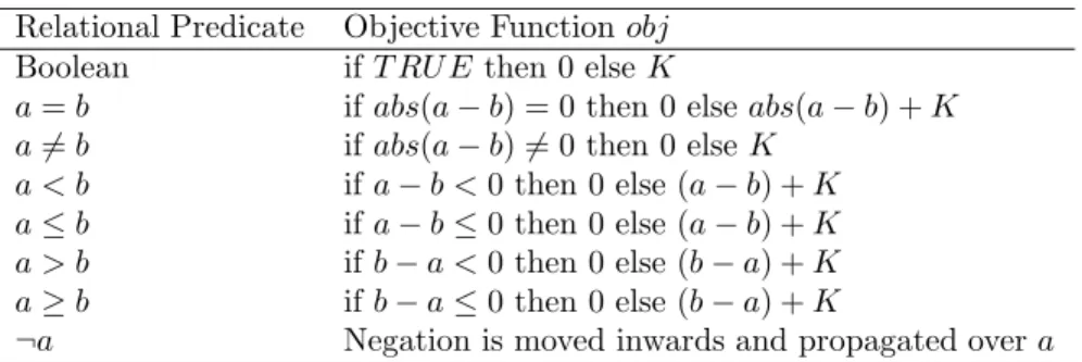
The objective function is simply the branch distance of the required branch when control flow diverges away from the intended path, or away from the target structure down a critical branch. The objective functions used (Table 2) are in principle identical to those employed by Korel, except the use of a non-zero positive failure constantK- which is always added if the branch predicate evaluates to false - removes the need to use a relationrelwithin the function. In this way, the objective function always returns a value above zero if the predicate is false, and zero when it is true.
In order to reduce the chances of the search becoming stuck in local op-tima, Tracey drops the constraint employed by Korel that the newly generated solution must conform to an already successful sub-path. However, the means of doing this results in the search losing some information about its progress. This is because solutions which diverge away from the target down earlier crit-ical branches are assigned similar objective values to those diverging away at a later stage. This can be demonstrated with the example of Figure 11. For the target statement at node 3, the false branches from nodes 1 and 2 are critical. Under Korel’s scheme, if the current solution is(i=10, j=-1), diverging down the critical branch from node 2, the vector (i=9, j=-1) would not be given consideration, because the already successful sub-path up to node 2 is violated. This is due to the fact that this input vector takes the earlier critical branch at node 1. However in Tracey’s method, a move can take place between solutions, and furthermore, the solutions are rewarded identical objective values - since the distance values taken at the different branching nodes are the same.
Relational Predicate Objective Functionobj
Boolean ifT RU Ethen 0 elseK
a=b ifabs(a−b) = 0 then 0 elseabs(a−b) +K a6=b ifabs(a−b)6= 0 then 0 elseK
a < b ifa−b <0 then 0 else (a−b) +K
a≤b ifa−b≤0 then 0 else (a−b) +K
a > b ifb−a <0 then 0 else (b−a) +K
a≥b ifb−a≤0 then 0 else (b−a) +K
¬a Negation is moved inwards and propagated overa
Table 2: Tracey’s objective functions for relational predicates. The value K,
K >0, refers to a constant which is always added if the term is not true
CFG Node
s void landscape_example(int i, int j)
{ 1 if (i >= 10 && i <= 20) { 2 if (j >= 0 && j <= 10) { 3 // target statement // ... } } }
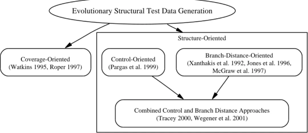
Structure-Oriented
Evolutionary Structural Test Data Generation
Coverage-Oriented (Watkins 1995, Roper 1997)
Branch-Distance-Oriented (Xanthakis et al. 1992, Jones et al. 1996,
McGraw et al. 1997)
Combined Control and Branch Distance Approaches (Tracey 2000, Wegener et al. 2001) Control-Oriented
(Pargas et al. 1999)
Figure 12: Classification of Dynamic Structural Test Data Generation Tech-niques using Evolutionary Algorithms
3.5
Applying Evolutionary Algorithms
The application of Evolutionary Algorithms to test data generation is often referred to in the literature asEvolutionary Testing(for example References [38, 39, 40]). The first work applying Evolutionary Algorithms to generate structural test data is that of Xanthakiset al. [41]. Up until this point, work on structural test data generation had largely focused on finding input data for specific paths or individual structures with programs, such as branches or statements. Initially, however, techniques using Genetic Algorithms took slightly different directions.
3.5.1 A Classification of Techniques
Different techniques applying Evolutionary Algorithms to structural test data generation can be categorised on the basis of objective function construction (Figure 12).
Coverage-Oriented Approaches reward individuals on the basis of covered program structures. In the work of Roper [42], an individual is rewarded on the basis of the number of structures executed in accordance with the coverage criterion. Under this scheme, however, the search tends to reward individuals that execute the longest paths through the test object . Guidance is not given for structures that are unlikely to be covered by chance, for example deeply nested structures, or branch predicates that are only true when an input variable has to be a specific value from a large domain.
The work of Watkins [43] attempts to obtain full path coverage for programs. The objective function penalises individuals that follow already covered paths, by assigning a value that is the inverse of the number of times the path has already been executed during the search. The direction of the search, there-fore, is under constant adaptation. However, the penalisation of covered paths, in itself, provides little guidance to the discovery of new, previously unfound paths. The results show that in comparison with Random Testing, the Genetic Algorithm approach required an order of magnitude fewer tests to achieve path
coverage for two experimental programs. However, both of these programs are of a simple nature, containing no loops. Furthermore, the input domains were artificially restricted for the search.
In general, the problem with coverage-oriented approaches is the lack of guidance provided for structures which are only executed with values from a small portion of the overall input domain. Therefore, it is difficult to expect full coverage with these techniques for any non-trivial program.
Structure-Oriented Approachesfollow similar lines to the earlier work of Ko-rel, and take a ‘divide and conquer’ approach to obtaining full coverage. A separate search is undertaken for each uncovered structure required by the cov-erage criterion. Structure-oriented techniques differ in the type of information used by the objective function. These can be categorised as either Branch-Distance-Oriented,Control-Oriented, orCombined approaches.
Branch-Distance-Orientedapproaches exploit information from branch pred-icates, in a similar style to earlier work by Miller and Spooner, and later Korel. In the work of Xanthakiset al. [41], Genetic Algorithms are employed to gener-ate test data for structures not covered by random search. A path is chosen, and the relevant branch predicates are extracted from the program. The Genetic Algorithm is then used to find input data that satisfies all the branch predicates at once, with the objective function summing branch distance values. However, this scheme suffers from similar problems suffered by the work of Miller and Spooner. Furthermore, the need to select a path is a burden on the tester. In the work of Joneset al. [44] for obtaining branch coverage, a path does not need to be selected. The objective function is simply formed from the branch distance of the required branch. However, no guidance is provided so that the branch is actually reached within the program structure in the first place. McGraw et al. [45] alleviate this problem for condition coverage, by delaying an attempt to satisfy a condition within a branching expression until previous individuals have been already found which reach the branching node in question. The initial generation for the target condition is then seeded with these individuals. This scheme, however, is inefficient if test data is required for the coverage of one, specific condition.
The earlier work of Korel had already removed the need for the tester to select a path. Since new test data considered by the search had to conform to the successful sub-path already found, explicit control-oriented information regarding the target did not need to be included in the objective function. However, such rigid constraints increase the chances of the search becoming stuck in local optima, and it would be better if more feedback could be provided via the objective function. This is the problem addressed by Control-Oriented
approaches.
WithControl-Orientedapproaches, the objective function considers the branch-ing nodes that need to be executed in some desired way in order to brbranch-ing about execution of the desired structure. The approach of Jones et al. [44] to loop testing falls into this category. Here, the objective function is simply the differ-ence between the actual and desired number of iterations. In the work of Pargas
et al. [46], for statement and branch coverage, the control dependence graph of the test object is used. The sequence of control dependent nodes is identified for each structure. These are the branching nodes that must be executed with a specific outcome in order for the structure to be reached. The objective value
-60 -40 -20 0 20 40 60 i -60 -40 -20 0 20 40 60 j 0 0.5 1 1.5 2
Objective Function Value
Figure 13: Objective function landscape of Pargas et al. [46] for example of Figure 11
of an individual is simply assigned as the number of control dependent nodes executed as intended. Recall that the branch leading away from the target at a control dependent node is identified as acritical branchin Korel’s work. The measure used by Pargaset al. is therefore equivalent to the number of critical branches successfully avoided by the individual.
The problem with using control information only for the purposes of the ob-jective function are the plateaux that form on the obob-jective function landscape. The objective function gives no guidance as to how to change the flow of execu-tion at control dependent nodes, since no distance informaexecu-tion is exploited from branch predicates. Take the simple example of Figure 11. The target is node 3, which is control dependent on node 2, which in turn is control dependent on node 1. Letdependent be the number of control dependent nodes for the cur-rent target, and executedthe number of control dependent nodes successfully executed in the required manner. A minimising version of the objective function of Pargaset al. , can be computed as (dependent−executed). However, in this scheme, every individual diverging away from the target at node 1 receives an objective value of 2, withevery individual diverging at node 2 receiving a value of 1. The landscape for the minimising version of the objective function for the example is seen in Figure 13. This landscape has three plateaux. For individu-als not satisfying one or more of the branch predicates, no guidance is given as to how to descend down the landscape to solutions that are closer to executing the target. Along these horizontal planes, the search becomes random.
infor--60 -40 -20 0 20 40 60 i -60 -40 -20 0 20 40 60 j 0 10 20 30 40 50 60 70
Objective Function Value
Figure 14: Objective function landscape of Tracey [47] for example of Figure 11
-60 -40 -20 0 20 40 60 i -60 -40 -20 0 20 40 60 j 0 0.5 1 1.5 2
Objective Function Value
Figure 15: Objective function landscape of Wegener et al. [48] for example of Figure 11
mation for the objective function. The work of Tracey [47] builds on previous work which used Simulated Annealing. The strategy for combining both tech-niques is as follows. The control dependent nodes for the target structure are identified. If an individual takes a critical branch from one of these nodes, a distance calculation is performed using the branch predicate of the required, alternative branch. This is computed using the functions of Table 2 (and Table 3 for and and or logical connectives). Tracey then uses the number of suc-cessfully executed control dependent nodes to scale branch distance values. Let
branch distbe the branch distance calculation performed at the branching node where a critical branch was taken. The formula used by Tracey for computing the objective function is:
executed dependent
×branch dist
Unfortunately, this scheme can lead to unnecessary local optima in the objective function landscape. For the example of Figure 11, this is evident by the valleys in the objective function landscape alongi= 9 and i= 21 where−3≤j and
j≥13, as seen in Figure 14.
Wegeneret al. [48, 38] map branch distance valuesbranch dist logarithmi-cally into the range [0, 1] (call this m branch dist). The minimising objective function is zero if the target structure is executed, otherwise, the objective value is computed as:
(dependent−executed−1) +m branch dist
The (dependent−executed−1) sub-calculation is referred to as the approx-imation level or, perhaps more appropriately, the approach level attained by the individual [48, 38]. The resulting objective function landscape has a similar form to that of Pargaset al. (Figure 15). However, the extra information pro-vided by the branch distance calculation prevents the formation of plateaux at each approach level. For the example, the result is a sweeping landscape from each level to the next level downwards.
3.5.2 Objective Functions for Different Structural Coverage Criteria
The work detailed so far for structural test data generation has mainly ad-dressed statement, branch or condition coverage. In the work of Wegener et al. [48], several new Structure-Oriented objective functions were introduced for previously unexplored coverage types. For this purpose, structural criteria are divided into four categories:
• node-oriented
• path-oriented
• node-path-oriented
• node-node-oriented
The basic form of the (minimising) objective function is:
The strategy in which approach level and m branch dist are computed varies according to the coverage type in question.
Node-oriented criteria aim to cover specific nodes of the control flow graph, for example statement coverage. The strategy for node-oriented methods was discussed in the last section. The approach level is calculated on the basis of the number of control dependent nodes for the target lying between nodes covered by the individual and the target node itself. At the point where control flow diverges down a critical branch, the branch distance is calculated using the predicate of the alternative branch.
Path-oriented criteria require the execution of specific paths through the control flow graph. There are two possible ways to calculate the objective function. One method is to calculate the approach level on the basis of the length of identical initial path section, with the branch distance calculation performed using the predicate at the first diverging branch. An alternative strategy considers all identical path sections for the approach level, with the branch distance calculation an accumulation of distance calculations made at each point of divergence from the intended path. Wegeneret al. report superior results with the latter method [48].
Node-path-oriented criteria include branch coverage and LCSAJ (linear code sequence and jump) coverage, where a node and a specific subsequent path must be executed. The objective function is a combined node-oriented and path-oriented calculation. Calculations for individuals not reaching the initial node are treated as for node-oriented criteria. For individuals reaching the initial node, a path-oriented calculation is additionally applied.
Node-node-orientedcriteria aim to execute a certain sequence of nodes through the control flow graph, without the specification of a concrete path between each node. This includes data-flow-oriented coverage types such asall-defs and all-uses criteria. In this case, the objective function is a cumulative node-oriented strategy. Calculations for individuals failing to reach the first node are carried out as for node-oriented methods, with individuals reaching the subsequent node having additional calculations carried out at these further nodes.
3.5.3 Control-Related Problems for Objective Functions
The provision of guidance to structures nested within loops presents a problem which can be demonstrated with Figure 16. The target is the execution of node 3. However, node 3 is not control dependent on node 2, because paths taking the false branch from node 2 can still execute node 3 in subsequent iterations of the loop. Consequently, the search does not receive guidance regarding the fact that the true branch from node 2 needs to be taken for the target statement to be reached. This results in poor search performance. The approach taken by Bareselet al. [49] is to treat branches that miss the target in iterations of the loop as if they were critical branches (recall that these branches are classed as semi-critical in Korel’s work). Thus, node 3 is treated as if it were control dependent on node 2. This also appears to be the approach taken by Tracey [47]. However, this leads to penalisation of individuals in the first iteration of the loop. In the example, if the input variableiis1, the objective value is taken in the first iteration, whennis0. However, the individual is closest to executing the target statement in the last iteration of the loop, whennis10. Furthermore, when the input value of iis 0, the individual will be deemed to have missed
CFG s 1 2 e 3 Node s void loop_example(int i) { int n; 1 for (n=0; n <= 10; n++) {