I
NTERNATIONAL
R
EAL
E
STATE
R
EVIEW
2004 Vol. 7 No. 1: pp. 1 - 30
The Chinese Housing Provident Fund
Richard J. Buttimer Jr.The Belk College of Business Administration, the University of North Carolina at Charlotte, Department of Finance and Business Law, 340B Friday Building, 9201 University City Boulevard, Charlotte, NC 28223-0001, (704) 687-6219, [email protected]
Anthony Yanxiang Gu
State University of New York, Geneseo, 115 D South Hall, 1 College Circle, Geneseo, NY 14454, [email protected]
Tyler T. Yang
IFE Group, 51 Monroe Street, Plaza E-6, Rockville, MD 20850, (301) 309-6561, [email protected]
The Chinese government has embarked upon an effort to reduce the number of tenants living in publicly owned housing. This is a significant challenge for any government, but may be especially so for a country where private homeownership is a new option. Out of concern that many of its citizens could not afford to purchase their housing units, the Chinese government created the Housing Provident Fund. This program, which is similar to housing fund programs in other countries such as Thailand and Singapore, combines a 401(k)-like savings and retirement account with subsidized mortgage rates and price discounts to provide a mechanism through which an employee could save for, and eventually complete, a housing purchase.
The housing provident fund (HPF) is very complex. It presents the participant with a number of options that can greatly affect their lifetime wealth. This paper presents a model of the HPF from the participating employee’s perspective, and then uses simulations to examine how the fund would affect the employee’s lifetime wealth under a variety of program parameters. From this information one can infer the optimal behavior for a rational program participant. It is also possible from the simulation results to infer which program parameters are the most likely to provide the best incentives to the employee to minimize the time that they stay in the program before they purchase their housing unit.
Keywords
provident fund, housing finance, China housing
Introduction
Since the early 1980’s, China has maintained two separate housing systems. The Chinese government established the first system in the early 1950’s. In that system, the government, government organizations, or state-owned enterprises directly own and allocate housing. In the second system, individuals privately own housing and trade it within a free market. During the past two decades the Chinese government has implemented a series of policies designed to privatize government owned housing.
Some of the difficulties that the Chinese government faces in this effort are similar to the difficulties that many Western governments face when privatizing public housing. One particular difficulty is that potential purchasers lack enough wealth to purchase the property outright, and they lack the income to make mortgage payments. To help alleviate this problem the Chinese government began a program under which it subsidizes savings for the purpose of purchasing formerly public housing. The purpose of this paper is to develop an economic model of the system, explore its comparative statics, and then illustrate its implications using a simulation model.
The outline of the paper is as follows. The next section describes the basic structure of the Chinese housing system with a particular focus on the operation of the public housing system. This section also discusses the difficulties that the Chinese government has had in privatizing public housing. The third section explains the details of the savings subsidy system implemented by the Chinese government. The fourth section presents a utility-based economic model of the system, while the fifth section presents simulation results that demonstrate the wealth effects the program would have on participants. Finally, the sixth section examines some policy implications of the model, summarizes and concludes the paper.
The Chinese Housing System
China has allowed the private development and ownership of housing since the early 1980’s, although the cost of privately owned housing has kept the
majority of Chinese citizens from purchasing their own property. Indeed,
many of the privately developed housing units either sit empty, or are purchased by companies and then provided to employees at subsidized rental
rates as part of their compensation package.2, 3For most Chinese citizens
living in cities their only real choice has been to live in state-owned housing. Historically the rent that the Chinese government charges for public housing has been below the cost to maintain the property, much less a market rental
rate.4 As a result, housing was largely allocated through non-price methods.
Usually the size and quality of the allocated housing was a function of the employee’s occupational rank, although seniority and family size also played a role in the allocation. For example, in 1998, a Senior Staff member in
Beijing5 would be assigned a 75 square meter apartment; a Section Director,
i.e., a manager with approximately 10 years work experience, would be assigned a 100 square meter apartment, and a Department Director, i.e. a senior manager with 20 years work experience, would be assigned a 150
square meter apartment.6 In all cases the rent paid by the tenant was trivial.
Rent and utilities accounted for 1.91% to 4.51% of household income from 1986 to 1997.7
During the 1980’s and into the early 1990’s, the government became increasingly unwilling and unable to continue the heavy subsidization of rents. The nation’s central government mandated that city governments phase in considerable rent increases. In fact, the central government required
rent to account for 15% of average household income by year 2000.8 For
example, in Shenyang rents were raised by approximately 30% annually from 0.15 Yuan per square meter of usable space per month to 1.98 Yuan per square meter in 2000. The Beijing city government raised its rent from
1.52 Yuan to 3.05 Yuan.9 It should be noted, however, that in some cases the
1 One could argue that there are other reasons beyond income constraints for this lack of
participation in the private sector housing market. Such reasons could include a lack of units, a lack of confidence in the willingness of the Chinese government to protect property rights, and a lack of economic sophistication on the part of potential housing owners. It is also very possible that the public housing is priced so far below an equilibrium market rent that it undercuts the private market. A thorough investigation of the reasons for this, however, is beyond the scope of this paper.
2 According to the 1999 State Statistical Bureau Statistics, in 1997 and 1998 the vacancy rate for
privately developed housing units was 51%.
3 People’s Daily, Overseas Edition, July 11, 1998. 4 Gu and Colwell (1997).
5 A senior staff member would normally be somebody with a College degree and at least five
years of work experience.
6 People’s Daily, Overseas Edition, November 16, 1998. 7 Statistical Yearbook of China, 1999
8 The State Council’s Decision on Further Urban Housing Reform, [1994] no. 43, July 18, 1994 9 Beijing City Government Housing Reform Office, Document 2000-080
increased rents were then at least partially offset by direct monthly cash payments from the government. For example, in Beijing the near doubling of rents was tempered by monthly cash subsidies of between 90 and 150 Yuan per month. For a Senior Director living in a 150 square meter apartment, their rent may have increased from 228 Yuan per month to 457, but, after factoring in the 150 Yuan cash subsidy, their real rent increased by only 79
Yuan per month.10
In 1990 the Chinese government began a program that encouraged occupants of public housing to purchase their homes. During 1998, the government announced that it intended to completely end the old housing allocation system. Although the Chinese government argues that up to 70% of the
urban public housing had been privatized by 2000,11 the privatization
program was not particularly successful in its early years. It was assumed that one reason for this lack of success was that Chinese citizens lacked the wealth to make a mortgage down payment and the income to make monthly payments.
It is probably unrealistic to believe that all residents of Chinese public housing will be able to eventually purchase their housing. Even in very affluent and developed countries such as the United States or Britain there are sizeable populations that lack the wealth or income to purchase their own housing and live in public housing. In a country such as China, where the social acceptability of wealth accumulation is not as strong, one might reasonably expect the percentage of the population living in public housing to be even higher. The Chinese government realizes, however, that one way to increase the home ownership rate is to increase the wealth level of those people that still live in publicly owned housing. To this end the Chinese government has created the housing provident fund, a savings program for housing purchases that also helps fund retirement for its members.
China is not alone in using a provident fund system to fund retirement and housing savings. A number of countries, including Singapore, India, and Thailand, have implemented such systems, with varying degrees of success. Although there are some common traits in each of these systems there are also significant differences among them in terms of their methods and goals. Some programs, such as the Chinese and Singapore plans, are compulsory for the majority of the population. Others, such as the Thai and Indian plans, are voluntary for large portions of the population. The Chinese and Indian 10 Ibid.
11 People’s Daily, Overseas Edition, March 30, 2000. We note that much of China’s rural
housing is still public, and it is not clear whether all of the housing that has been privatized has been sold to individuals, or if some of it has been transferred to the balance sheet of other state affiliated institutions.
programs pay a fixed rate of return on funds invested in the program; the Singapore and Thai plans allow the individual to invest in a variety of asset classes, including annuities, stocks, bonds, and gold.
Perhaps the most common trait among these plans, however, is their complexity. The programs require their members to make very sophisticated financial decisions, and endow their participants with a variety of choices. The next section describes the program in China in detail.
The Housing Provident Fund System
The housing provident fund was initially introduced as a pilot program in Shanghai in late 1991, and was extended nationwide in 1995. The program is open to employees of government agencies, state enterprises, universities, hospitals, and some semi-state companies. Recently the government has mandated that all eligible employees must join the program, although privately employed workers do not have to participate.
An employee that joins the program agrees to have between 4% and 10% of their salary deposited into a special account in a state owned bank. While this account only pays the risk-free interest rate, the participant’s employer provides a one-for-one match for each Yuan that the employee deposits into the account. These employer-matching funds are deposited into the same account and they also earn the risk-free rate. The employee owns the account, and all money in it, although they can only use the funds for the purchase of
housing.12 Should the employee die, their funds become part of their estate.
Once in the program, however, the employee must continue their monthly contributions to their HPF account until they retire, pass away, or are separated from their employer. The employee may not voluntarily withdraw from the program while they are still employed by the state or state-sponsored entity. Except for not being able to withdraw from the program, this savings component of the system is very similar to 401(k) or IRA retirement programs in the United States.
In addition to the employer-match, participants in the system also have the right to purchase the state-owned housing they occupy at a discount relative to the price the government would charge non-participants. Depending upon the employee’s rank, job tenure, job performance, and other factors, the price of the property will range between 10% and 40% of the government’s 12 Upon the retirement, the employee can withdraw the entire account and use it for other
purposes. Upon the death of the employee, their heirs have the same access to the funds that a retired employee would have.
normal asking price. Interestingly, the program does allow the employee the opportunity to purchase housing that is better or larger than that to which their rank entitles them. In such a case the price the employee pays a discounted price for that portion of the unit to which they are entitled by rank, and the full price for the “extra” portion. For example, if a Section Director were entitled to a 100 square-meter unit but instead purchased a 150 square-meter unit, they would pay the discounted price on the first 100 meters of the unit and the full price on the remaining 50 square-meters.
If an employee is renting a unit and separates from their employer, they must either vacate the unit or pay a higher rental rate on it. If, however, they have purchased the unit, it is their property to keep. The employee may chose to continue living in the property, but they may also sell the property in a free market. While originally there was a five-year blackout period on reselling the property, that constraint was eliminated in 1997 in Shanghai, followed by almost all cities by 2001.
The government uses two additional financial subsidies to encourage participation in the system. First, participants in the program are able to acquire mortgages at below market rates from State-owned banks. Second, the government waives a 10% tax normally required on housing transactions;
effectively further reducing the cost of a unit by 10%.13
A Utility-Based Model of Consumer Choice
The housing provident fund (HPF) system is very complex, and requires its participants to make some very sophisticated financial decisions. Indeed, in one sense the decision as to whether or not to join HPF is not trivial. Even though, as mentioned earlier, it is now mandatory for currently eligible employees to join, a worker just entering the workforce implicitly decides to join the HPF when they accept government employment. If they were to decide to accept only private employment they could avoid joining HPF. While modeling the worker’s decision whether or not to take public employment is beyond the scope of this paper, we do use the idea that an
individual could avoid HPF to establish our base economic case.14
13 The Peoples Daily, Overseas Edition, October 30, 1999.
14 There is a well-established literature that examines housing consumption over the life cycle.
Examples include Artle and Varaiya (1978), Kan (1999), and Kan (2000). That literature, however, generally is concerned with housing choice under where the primary constrain is a person’s budget and preference set. This paper specifically focuses on the incentives that the HPF program provides, and so uses a more narrowly defined method for analyzing the problem. For example, Kan (1999) considers the problem of mobility and how it affects housing choice.
Even after an employee has joined HPF they still have a significant decision to make: when to actually purchase their housing. In the extreme case, an HPF participant could delay the purchase of housing indefinitely; in such a case they would essentially treat the program as a retirement fund.
The government must concern itself with these choices as well. Under the assumption that renters are unlikely to ever accumulate enough wealth to purchase their housing units without the HPF program convincing tenants to join is a necessary condition for eventually reducing or eliminating the government’s ownership of housing. It is not, however, a sufficient condition, as the tenant must still decide exactly when to purchase the housing. During this interim period between the employee joining the HPF and purchasing their housing unit, the cost to the government is quite high given that the consumer continues to receive their rent subsidy and they also receive the savings subsidy. Clearly the government has an interest in reducing this time period.
The model begins with the assumption that the employee maximizes lifetime utility, and that the marginal benefit to the employee of the HPF program is the difference in their total expected utility under the program compared to their total expected utility if they were not in the program. That is, it compares their total expected utility under HPF with what their utility would be if they were able to simply live in public housing with subsidized rental rates for the rest of their lives.
Before building the model we must make a fundamental choice as to how we will proceed: we must decide whether we will work within a stochastic or deterministic framework. Although it is tempting to use a stochastic framework, we chose to work within a deterministic framework for a couple of reasons. First, the number of variables that we would have to treat as
stochastic is prohibitively large.15 Given that we are unlikely to find
closed-form solutions for our model, we are limited to solving it through numerical methods and generally numerical methods work for two or three stochastic state variables, but become untenable for larger numbers. Second, we wish to build as complete a model as possible so that we can determine which variables are the most important factors in the model. If we were to treat a subset of parameters as stochastic while treating the rest as deterministic we would necessarily limit the scope of the model, and inappropriately shift the focus of the model onto just a few parameters.
We agree that mobility is an issue, but it is not one that directly relates to the HPF incentives that we wish to examine, and so we implicitly assume that the HPF participant is not mobile.
15 At a minimum we would have to treat interest rates, house prices, employee income, market
The lifetime utility maximization problem is given by:
(
)
, , , , Max { },{ }, { },{ } 0 s.t. ( ) 0 0 t t T H t C t H t t C t t T t T U H C B t P P T T P H P C t B y W ∂ ∫ + ∂ + ≤ + ∫ ∫⎛
⎞
⎜
⎟
⎝
⎠
0(1)
where U(.) is the employee’s utility function, Ht is their housing
consumption at time t, Ct is their non-housing consumption at time t, BT is
the amount of bequest left for their heirs upon death, PH,t is the housing price
at time t, PC,t is the price of other goods at time t, yt is the employee’s income
at time t, and W0 is the employee’s initial endowment.
Within this utility framework, the house price and mortgage interest rate subsidies that the HPF provides are equivalent to reducing the price of housing for the employee. Usually reducing the price of a good can lead to either price or substitution effects (or both). In this case, however, recall that the reduction in housing price is only on the unit that the consumer already occupies, not on any larger space, so, at least in the short run, there is
effectively no substitution effect.16 Instead the increased income can be used
to increase the consumption of other goods or it can be used to increase their savings and eventually the bequest that they make to their heirs. The leaving of an inheritance is especially important in Chinese culture, and increasing the size of the bequest is given a heavy weighting in a consumer’s utility function.
Since the consumer maximizes their expected utility, they will elect to redistribute their income to their highest marginal utility use. For tractability the model assumes that increasing marginal consumption provides no more marginal utility for the consumer than does increasing the marginal bequest (i.e. savings). This allows the model to express the benefits of the HPF relative to renting in terms of the present value of net savings, i.e. the
increase in the present value of the future bequest.17 Given this assumption,
the decision whether or not to join the HPF becomes a rent versus buy decision, albeit a very complex one.
16 It is possible the consumer will elect to use the “saved” money to purchase additional housing
units at the higher price, but this is really more of an income effect; they are changing their consumption bundle because they have additional money since the cost of housing they already occupy has changed, not because the price of the marginal unit of housing has changed.
17 This future bequest amount will include any anticipated growth in the value of the housing
itself. The consumer will have incentives to maintain and even increase the quality of the housing to maximize future appreciation in the property. This may well provide a positive externality relative to renting since renters have no incentive to maintain their property.
The model uses the following variables:
Ht = market house price at time t;
Rt =rent of the same house set by the government at time t;
Mt =housing maintenance cost at time t;
yt =employee’s income at time t;
T =expected time of house sale at maturity of the mortgage loan or
lifetime of the participant, T–τ = mortgage term;
rs =government-subsidized mortgage rate for HPF participants;
rf =bank deposit rate, used to discount cash flows and estimate interest
earned on the housing saving account;
gH =house price growth rate;
gM =maintenance cost growth rate;
gR =rent growth rate;
gY =income growth rate;
Ft=balance in participant’s HPF account at time t;
α =percentage of house price to be paid when purchasing housing under
the program;
β =percentage of employee’s income required to contribute to the
housing fund;
D=down payment as percentage of purchasing price required in
purchasing housing under the program;
DP=Cash amount of down payment;
τ =time of the housing purchase under the program;
ξ=the ratio of government’s contribution to employee’s contribution to
the housing fund account;
W0=the initial wealth of the participant.
A Measure of Lifetime Utility
The model assumes that the employee’s utility is monotonically increasing in net present wealth, and the employee’s income from their job remains the
same regardless of whether or not they join HPF.18 The key to the model’s
analysis is that it treats renting as a pure cost to the employee, but recognizes that expenditures under HPF can have both a cost and an investment aspect to them. It is the investment aspect of the HPF program that complicates the measurement of the employee’s utility. Any measure must take into account both the additional costs of the HPF program as well as the potential returns 18 This assumption allows us to avoid the consumption-smoothing problems like those discussed
in Leung and Tse (2001) or Tse and Leung (2002). If we only maximized current utility then when the employee joined the program they might have an initial utility reduction, due to the cash flow lost by joining the program forcing them to reduce consumption. Since the consumer is maximizing net present wealth, however, the loss in immediate consumption is compensated by an increase in future consumption.
it provides. This model measures the employee’s utility by measuring the net present value of the wealth that they have available to spend on goods other
than the housing unit they would have had had they continued to rent.19 By
focusing on the other income that the employee has to spend, the model is able to isolate how the HPF program affects the employee’s true cost or benefit of participating in the system.
The model defines the variable NHWRent as the wealth available for
non-housing goods under the rental system:20
NHWRent = PV lifetime income – PV rental expenditures,
and the variable NHWHPF as the wealth available for non-housing goods
under the HPF system:
NHWHPF = PV lifetime income – PV HPF expenditures (3)
Under HPF the expenditures can be either positive or negative. If they are positive, they represent a cash outflow to the employee and are a reduction in the income they have available to spend on non-housing goods. If they are negative they represent a cash inflow to the employee and increase the income that they have available to spend on non-housing goods. One source of such a negative expenditure, for example, would be capital gains on the purchased housing unit.
Given Eqs. (2) and (3), the model can calculate the net present benefit of the HPF program to the employee:
Net present benefit =NHWHPF – NHWRent (4) Since the model assumes that lifetime income is equal regardless of the employee’s decision to join or not join HPF, some simple algebra reveals that the determinant of the participant’s net marginal benefit is equal to the net present differences in the housing expenditures under renting and HPF: Net present benefit = PV rental expenditures – PV HPF expenditures (5) Equation (5) is the basic equation the model uses to examine the effects of joining HPF. The following sections examine the specific equations used to construct the various sub-components of this equation.
19 This wealth available to spend includes income they spend on any additional square footage of
housing they elect to purchase under the HPF system.
20 Again, these non-housing goods would include additional square footage purchased under
Lifetime Income
The model assumes that there are two potential sources of income available to the employee, regardless of their HPF status: their salary income and their
initial wealth.21 Working within a continuous time framework the present
value of initial wealth and salary income is given by:
( )
(
)
0 0 t 0 0 e 1 Lifetime income e Y f f g r T T r t Y f t Y W y t W g r − − = − = + ∂ = + −∫
(6) Rental ExpendituresIf the employee were not in the HPF system they would continue to pay the government-set rent for the remainder of their life. This does assume that there will always be rental housing available.
Working within a continuous-time model, this results in a lifetime present value of the housing expense as:
( ) 0 0 (e 1) Rental expenditures e R f f g r T T r t t R f t R R t g r − − = − = ∂ = −
∫
(7) HPF ExpendituresEvaluating the lifetime expenditures of the consumer under the HPF program is much more complex. One must consider the combined rental and savings cash flows between the time when the employee enrolls in the program and when they actually purchase their house. One must consider mortgage and maintenance costs after the consumer purchases the house, as well as the sales value of the house, and the effect that these capital gains have on their bequest. It is possible to combine these into a single equation that is the HPF analog to Eq. (7): the net present expenditures of joining HPF:
21 Recall that any income generated by participating in HPF will be treated as a negative HPF
[
]
0 ( ) ( ) HPF expenditures ( )e ( )e ( ) e ( ) e e (1 ) e e s.t. f f f f f f f T r t r t t t t t t t T s r t r T T t T r T r T t r T t t R y t y M t H DP r t H H DP F y t τ τ τ τ τ τ τ τ β β α α β ξ τ θ − − = = − − = − − − = = + ∂ + + ∂ + − ∂ − − − − + + ∂ ≥⎡
⎛
⎞⎤
⎜
⎟
⎢
⎥
⎣
⎝
⎠⎦
∫
∫
∫
∫
(8)where each element has the following meaning:
• The first element (
0 ( )e r tf t t t R y τ β − = t + ∂
∫
) is the rent and contributionto the housing fund account prior to the purchase of the house,
• The second element ( ( )e f
T r t t t t y M t τ β − = + ∂
∫
) is the continuingcontribution to the housing fund and the maintenance expense occurred after the purchase of the house,
• The third element ( ( ) e f
T s r t t Hτ DP r t τ α − = − ∂
∫
) is the interest paymentsfor the loan22,
• The fourth element ( ) is the proceeds
from selling the house less the repayment of the loan
[
( ) r Tf T H − αHτ −DP]
− e e f t −23, and
• The last element ( )
represents the refund of unused employee contribution to the housing fund account upon exiting of the program, either upon retirement or death. ( ) ( ) ef (1 ) e f T r T r T t r T t t Fτ τ y τ β ξ − − = + + ∂
⎡
⎛
⎞⎤
⎜
⎟
⎢
⎥
⎣
⎝
∫
⎠⎦
There are a few constraints that must be imposed upon this equation. First, θ
is the minimum time required to accumulate enough cash in the account to 22 For simplicity the model assumes an interest-only loan. One could easily incorporate an
amortizing loan, but doing so adds nothing to the analysis and requires the addition of a new time parameter – the maturity date of the mortgage.
23 If one is uncomfortable with the idea that the participant is “forced” to sell the house a time T,
one can alternatively interpret this as the net capital gain (less the mortgage balance) earned on the house as of the participant’s maturity horizon. We thank an anonymous referee for providing this interpretation.
be able to make the down payment. If this is based upon a percentage of the sales price, it is the time that makes the following statement true:
∂
⎟
( ) 0 (1 )erf t t t DH y t θ θ θ α β ξ − = =∫
+ (9)Recently, the Chinese government has stopped requiring a specific down payment percentage, and has simply stated that after six months in the program HPF participants are eligible to purchase using whatever funds are
in their account for their down payment. In such a case θ is simply set equal
to six months.
While θ is the minimum time that the employee must remain in the program
in order to purchase their housing, the employee could stay in longer before making their purchase. In theory a person staying in the program for a sufficiently long period of time could accumulate more money in their account than is required to purchase their housing outright, i.e. without a mortgage. The model assumes, therefore, that upon the purchase of their housing the HPF participant will use all funds in the housing account, up to the price of the house, as their down payment. Thus the down payment (DP) made at a time τ>θ is given by
( ) 0 min (1 )erf t , t t DP y t H τ τ τ β ξ − α = =
⎛
⎜
+ ∂⎞
⎝
∫
⎠
(10)The balance of the housing fund after the down payment is made is ( ) 0 max 0, (1 )erf t t t F y t τ τ τ β ξ α τ − = =
⎛
⎜
+ ∂⎞
⎝
∫
− H⎠
⎟
(11)Marginal Benefit of Joining HPF
From Eq. (5) the differences in the marginal utility of the employee from joining HPF is the difference in the expenditures, thus the net marginal benefit is given by:
(12) T f r
[
]
( ) ( ) sNet marginal benefit e ( )e
0 0 ( )e ( ) e ( ) e e (1 ) e e t t t t T T T t f f t t t f t t f f T f f t T r r R t R y t t t T r y M t t T r H DP r t t r H H DP T r r F y t t τ τ τ τ τ β β τ α τ α β ξ τ − − − − = ∫ ∂ − ∫ + ∂ = = − − ∫ + ∂ = − − ∫ − ∂ = − + − − − + + ∫ + ∂ =
⎡
⎛
⎞
⎤
⎜
⎟
⎢
⎝
⎠
⎥
⎣
⎦
From Eq. (12), it is clear that the housing saving program is a collection of several different subsidy components. Implicit in Eq. (12) is the assumption that the HPF program and its subsidies will remain in place for the entire time horizon of the participant. One can reasonably question the ability and willingness of the Chinese government to maintain this program and its subsidies if the entire Chinese population were to elect to join the program. If the model were to allow for the potential that the program could disappear in the future because its popularity precluded the Chinese government from continuing its subsidies, this would alter the decisions of the participant with respect to when they would exercise their purchase option. Doing so, however, would require a general equilibrium model like that of Gervais (2002), and would not let us address the primary goal of this paper: to determine the incentives facing the participant under the program as it now stands.
The model can be used to assess the marginal contribution of each component with respect to the employee’s decision. This also provides a measure of the relative effect of each of the various subsidy policies. Table 1 presents the signs of the various partial derivatives.
The partial derivatives in Table 1 provide insights as to how the program will affect the wealth of the participants. For those components with positive derivatives, increasing the value of the factor will increase the employee’s marginal wealth under the program. For those factors with a negative first partial derivative, increasing that aspect of the program will decrease the participation in the program. Not surprisingly, the negative partials stem from costs that the participant must bear (i.e., housing price, mortgage amount, etc.) under the system.
Table 1: Comparative statics for net marginal benefit (NMB) from participating in program 0 0 0 0 0 0 NMB NMB NMB H R D ∂ ∂ ∂ > < > {< ∂ ∂ ∂ 0 0 y 0 0 NMB NMB NMB G α τ ∂ < ∂ > ∂ {> < ∂ ∂ ∂ 0 0 0 0 0 R NMB NMB NMB M β G ∂ ∂ ∂ > < > {< ∂ ∂ ∂ 0 0 0 0 H NMB NMB NMB y ξ G ∂ ∂ ∂ > > ∂ ∂ ∂ >
These partial derivatives by themselves, however, do not provide enough information to fully analyze the benefits of the program from the perspective of either the participant or the government. Recall that a primary objective of the HPF program is to provide a mechanism through which the government can privatize public housing. A reason for this is that the rental rate is subsidized so heavily that rental income does not even cover maintenance costs. Presumably, the government wishes to incite the HPF participant so as to minimize the time between their joining and their purchase of the housing unit. There are also several partial derivatives with an indeterminate sign. For those factors, the impacts would depend upon the values of specific parameters. To address these issues, the next section numerically solves the marginal benefit equation for a variety of parameter values.
Numerical Examples
Some numerical examples may help illustrate the implications of the above model. In these examples we uses parameters that are representative of the Chinese economy and housing market and that best allow illustration of the effect that HPF participation has on the employee’s utility. The model then conducts sensitivity analyses around these base conditions to illustrate the potential impacts of changes in either market conditions or the conditions of the program.
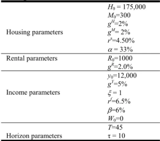
Table 2 lists the parameters the base case simulation uses. One can classify the parameters as fitting into four groups: those relating to the cost of renting, those relating to the cost of purchasing the housing unit and its financing, those relating to the employee’s income and the structure of the program, and those relating to the timing of the employee’s decisions.
Table 2: Base parameter values for simulations Housing parameters H0 = 175,000 M0=300 gH=2% gM= 2% rs=4.50% α = 33% Rental parameters R0=1000 gR=2.0% Income parameters y0=12,000 gY=5% ξ = 1 rf=6.5% β=6% W0=0 Horizon parameters T=45 τ = 10
There are six parameters relating to the cost of purchasing the housing unit.
The first is the initial cost of the house at time 0, H0. It has a base value of
175,000 Yuan. The base growth rate for housing costs, gH, is set to 2%. The
initial maintenance costs, M0, are 300 Yuan per year, and their growth rate,
gM, is initially set to 2%. Both the value of H
0 and M0 are set to values that
are in line with published values for those parameters.24 The two final
parameters that directly affect the housing purchase cost are the percent of
the market price that the employee must pay, α, and the subsidized mortgage
rate, rs. These parameters are set to 33% and 4.5% respectively. The value
for α is set by the program but could vary according to the employee’s rank
and tenure with the enterprise, and the subsidized mortgage rate has been steadily in the 4.5% range over the past several years.
The two rental parameters are the initial rental rate R0 and its growth rate gR. These parameters are set to 1000 Yuan per year and 2%, respectively. The initial rental rate is consistent with that of a very junior employee. The model sets the growth rate in the rental rate to be equal to the growth rate in housing prices under the theory that in the long run rental price increases should closely mirror increases in housing prices. In some of the simulations the model relaxes this assumption and allows the rental growth rate to be considerably higher than that of the housing growth rate, to simulate the effect of the government increasing the rental rate at an artificially high speed as an incentive to participants to purchase their housing.
There are six income-related parameters in the model. The initial income level, y0, is set to 12,000 Yuan per year, and the income growth rate, gY, is set to 5%. The risk-free rate, which is the rate paid on the HPF account, is set to
6.5%, which is consistent with the Chinese risk-free rate in the recent past. One can see from this that the government does heavily subsidize the HPF
mortgage rate, rs, which is 4.5%. The employer match of HPF employee’s
funds contributions, ξ, is set to 1 and the mandatory contribution from the
employee is 6%. Both of these parameters are the values the program currently uses. The initial wealth of the participant, W0, is set to 0. Since this parameter appears on both sides of Eq. (5), it simply washes out and one can set it to 0 without loss of generality.
The final two parameters relate to the horizon of the employee. The
parameter T is the time before the employee exits the HPF program in its
entirety and liquidates all of their assets. The model assumes this happens
upon the retirement of the employee. The base value for T is 45 years, which
corresponds to the horizon for a 20 year old beginning their career. The
second horizon parameter is τ, the date when the employee purchases their
housing unit. Although this parameter has a base value of 10 years, in each
of the simulations the model examines a variety of values for τ.
When considering these parameter values, one must keep in mind that the purpose of these simulations is not to precisely replicate the Chinese economy or to provide a robust estimate of the value of the HPF program to a particular employee. Rather, they are conducted to illustrate the relative effects of each parameter on employee wealth, and to do so using values that are of the appropriate scale for the HPF program and for the Chinese economy.
Simulation Results
Base Case
Using the base parameter set, the net present benefit for the HPF participant
is 24,175 Yuan, which is slightly more than 2 times the initial base salary, Y0,
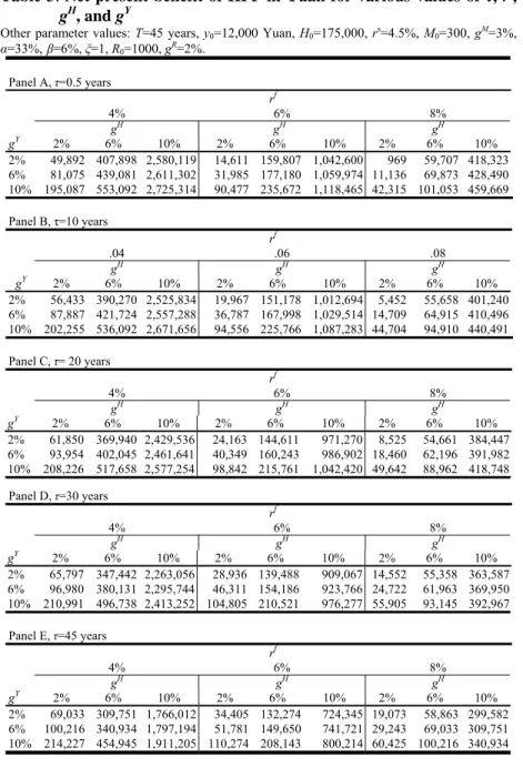
of 12,000 Yuan. One value, of course, presents only a very limited view of the model. To present a more complete view, Tables 3-6 demonstrate the net present benefit to the participant under a variety of parameter combinations and with differing times until the participant purchases their house.
Table 3: Net present benefit of HPF in Yuan for various values of τ, rf, gH
, and gY
Other parameter values: T=45 years, y0=12,000 Yuan, H0=175,000, rs=4.5%, M0=300, gM=3%,
α=33%,β=6%, ξ=1, R0=1000, gR=2%. Panel A, τ=0.5 years rf 4% 6% 8% gH gH gH gY 2% 6% 10% 2% 6% 10% 2% 6% 10% 2% 49,892 407,898 2,580,119 14,611 159,807 1,042,600 969 59,707 418,323 6% 81,075 439,081 2,611,302 31,985 177,180 1,059,974 11,136 69,873 428,490 10% 195,087 553,092 2,725,314 90,477 235,672 1,118,465 42,315 101,053 459,669 Panel B, τ=10 years rf .04 .06 .08 gH gH gH gY 2% 6% 10% 2% 6% 10% 2% 6% 10% 2% 56,433 390,270 2,525,834 19,967 151,178 1,012,694 5,452 55,658 401,240 6% 87,887 421,724 2,557,288 36,787 167,998 1,029,514 14,709 64,915 410,496 10% 202,255 536,092 2,671,656 94,556 225,766 1,087,283 44,704 94,910 440,491 Panel C, τ= 20 years rf 4% 6% 8% gH gH gH gY 2% 6% 10% 2% 6% 10% 2% 6% 10% 2% 61,850 369,940 2,429,536 24,163 144,611 971,270 8,525 54,661 384,447 6% 93,954 402,045 2,461,641 40,349 160,243 986,902 18,460 62,196 391,982 10% 208,226 517,658 2,577,254 98,842 215,761 1,042,420 49,642 88,962 418,748 Panel D, τ=30 years rf 4% 6% 8% gH gH gH gY 2% 6% 10% 2% 6% 10% 2% 6% 10% 2% 65,797 347,442 2,263,056 28,936 139,488 909,067 14,552 55,358 363,587 6% 96,980 380,131 2,295,744 46,311 154,186 923,766 24,722 61,963 369,950 10% 210,991 496,738 2,413,252 104,805 210,521 976,277 55,905 93,145 392,967 Panel E, τ=45 years rf 4% 6% 8% gH gH gH gY 2% 6% 10% 2% 6% 10% 2% 6% 10% 2% 69,033 309,751 1,766,012 34,405 132,274 724,345 19,073 58,863 299,582 6% 100,216 340,934 1,797,194 51,781 149,650 741,721 29,243 69,033 309,751 10% 214,227 454,945 1,911,205 110,274 208,143 800,214 60,425 100,216 340,934
The Effects of Housing and Income Growth Rates
Table 3 presents the result of varying four parameters, τ, rf, gH, and gY
, from their base parameter values. These parameters are the ones that most directly affect the employee’s income, the cash they accumulate in their housing fund, and the house value. Table 3 consists of five panels, each with a different
value of τ. In Panel A, τ is set to six months, meaning the employee
purchases the house as soon as they are eligible to do so under the program. In Panel B, τ is set to 10 years, in Panel C it is set to 20 years, in Panel D it is 30 years, and in Panel E it is set to the maximum at 45 years. Panel E corresponds to the situation where the participant purchases their house at the moment they retire; they essentially treat the HPF as a retirement account. They never purchase the house to live in, but rather only purchase it and immediately resell it upon their exiting the HPF program. Since the
government will sell the housing units at the price αHT, and presumably the
employee can resell it immediately at HT, the model assumes they act
rationally and exploit the arbitrage.
Table 3 varies the other parameters within each panel. The risk free rate, rf,
is set to 4%, 6%, and 8%. The housing growth rate, gH, is set to 2%, 6%, and
10%, and the income growth rate, gY, is set to 2%, 6%, and 10%.
It is clear from Table 3 that the parameter that is most influential to the
participant’s net present benefit is the housing growth rate, gH. For example,
in Panel A, with rf set to 4% and gY set to 2%, changing gH from 2% to 10%
results in the participant’s wealth increase changing from 49,892 Yuan to 2,580,119 Yuan.25 Similarly, if rf is set to 8%, and gY is held at 2%, changing
gH from 2% to 10%, results in the participant’s wealth increase changing
from 969 Yuan to 418,323 Yuan. Panels A, B, C, and D of Table 3 demonstrate that increasing the housing growth rate monotonically increases the participant’s wealth.
Increasing the risk-free rate has two effects on a HPF participant. The first effect is that it increases their earnings on the HPF account, thus reducing
the size of the mortgage they must use for a given τ value. The second effect
is that all of the cash flows are now discounted at a higher rate, which reduces the present value of the future benefits of the HPF. Given that some of the most valuable benefits of HPF occur very far in the future, this effect can be significant. The results in Table 3 show that holding everything else
constant, increasing rf will reduce the wealth of the employee. For example,
25 At first glance the net present benefit of 2,580,119 Yuan is startling. One must keep in mind,
however, that nearly all of this value comes from the increase in the house value. Note that under a continuous compounding rate of 10%, a house that has an initial value of 175,000 Yuan would be worth 9,554,676 Yuan after 40 years.
in Panel A, with rf equal to 4% and gY and gH set equal to 2%, increasing rf
from 4% to 8% results in a decrease in the net present benefit of joining HPF
from 49,892 Yuan to 969 Yuan. Similarly, with gYand gH each set at 10%,
increasing rf from 4% to 8% results in a decrease in the net present benefit of
joining HPF from 2,725,314 Yuan to 459,669 Yuan.
One parameter that the employee controls is τ, so it is interesting to examine
how various values of τ can affect the employee’s net present benefit. This is
a way of examining the employee’s optimal holding period for their option
to purchase the house.26 Reading vertically across panels allows one to
examine this issue. For example, increasing τ from 0.5 year to 45 years,
given values for rf, gY, and gH of 4%, 2%, and 2%, respectively, results in the
employee’s net present benefit increasing from 49,892 Yuan to 69,033 Yuan. Given that the growth rate in housing is so low, the employee is better off delaying their purchase of housing for as long as possible and continuing to
earn the higher risk free rate of return. On the other hand when gHis greater
than rf, the employee is better off purchasing the housing as soon as possible.
This can be seen by increasing τ from 0.5 year to 45 years when rf, gY, and
gH have values of 4%, 10%, and 10%, respectively. In this case the net
present benefit is 2,580,119 Yuan when τ is 0.5 years and only 1,911,205
Yuan when τ is 45 years. This basic pattern – delay purchasing when gHis
low and purchase as soon as possible when gH is high - repeats regardless of
whether gY is high or low.27
Perhaps the most intriguing result in Table 3 is when gH is set to be slightly
less than rf, i.e. when gH=6% and rf=8%. Regardless of the gY value, the HPF
participant’s Net Present Benefit is roughly equal when τ is either set to .5
years or 45 years, but follows a U-shaped pattern for τ values of 10, 20 or 30
years. The risk free rate is not large enough to allow it to dominate the growth rate housing in the early years: it takes many decades for the risk-free rate’s higher value to overcome the initial advantage that immediate purchase provides due to the subsidized house purchase price. This means that for employees with a shorter time horizon (i.e. older employees) that immediate purchase is optimal, but that employees with a longer time horizon (i.e. younger employees) will be indifferent between immediate purchasing their housing and delaying their purchase for a very long time.
One implication that can be drawn from Table 3 is that the employee’s expectations regarding the future growth rate of housing may be more 26 One must solve for the optimal holding period numerically.
27 We note that when analyzing these results we place to constraints on the employee – a
minimum purchase time (τ=0.5 years) and a maximum purchase horizon (τ=45 years), so that when we discuss an optimal time to purchase we necessarily mean a constrained optimum. This causes many of our results to be corner solutions.
important in their decision as to when they purchase their housing than is their perception as to the growth rate in their salary. In other words, the optimal behavior of the employee is determined by the relative attractiveness of housing as an investment, not by its affordability in terms of the
employee’s income.28
The Effects of the Income Match and the House Price Discount
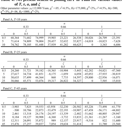
The HPF program contains various discounts and subsidies for participants. Two of the most important such benefits are the matching of the employee’s contribution by their employer and the discount on the house price they get for participating in the HPF. Table 4 examines the relative effect of these benefits on the employee’s net present benefit, and how that might affect the employee’s decision as to when to make their purchase.
Specifically, Table 4 examines the effects that four parameters, τ, T, α, and ξ,
have on the employee’s net present benefit. Recall that α is the percentage of
the housing unit’s “market” price that the employee must pay under HPF,
and ξ is the rate at which the government matches the employee’s HPF
contributions. These two parameters provide mechanisms through which the government can reduce the cost of the housing and increase the employee’s
wealth. The effect of α on the employee’s wealth ends at time τ, when the
participant purchases their housing unit; the effect of ξ, however, depends on
both τ and T. It depends upon τ because ξ and τ jointly determine the amount
of cash the employee will have to make a down payment.29 It depends upon
T since the employee must continue to make contributions to HPF even after
they purchase the housing unit. Table 4 consists of three panels that are
characterized by differing time horizons T, for the investor. Within each
panel are various net present benefit values for combinations of τ, α, and ξ. The most striking feature of the results in Table 4 is that for many parameter combinations the net present benefit is negative, indicating that it is a net wealth loss for the employee to join HPF. Presumably the employee would not join HPF if they had the option of not joining. This does raise the issue of whether the Chinese government’s decision to mandate participation in the program was in the best interest of all participants.
28 There is obviously a lower limit to this, since the homeowner must be able to make the basic
mortgage payments.
29 For a given set of values of rf, y
Table 4: Net present benefit of joining HPF in Yuan for various values of T, τ, α, andξ
Other parameter values: y0=12,000 Yuan, gY =.05, rf=6.5%, H0=175,000, gH=2%, rs=4.5%, M0=300,
gM=3%, β=.06, R 0=1000, gR=2%. Panel A, T=10 years α 0.33 0.66 1 ξ ξ ξ τ 0 0.5 1 0 0.5 1 0 0.5 1 0.5 68,364 71,682 74,999 19,903 23,221 26,538 –30,026 –26,709 –23,391 5 71,614 74,809 78,004 29,437 32,632 35,827 –14,018 –10,823 –7,628 10 74,762 78,105 81,448 37,939 41,282 44,625 0 3,343 6,686 Panel B, T=25 years α 0.33 0.66 1 ξ ξ ξ τ 0 0.5 1 0 0.5 1 0 0.5 1 0.5 24,260 31,721 39,182 –18,365 –10,904 –3,443 –62,282 –54,821 –47,360 5 27,617 34,734 41,851 –8,175 –1,059 6,058 –45,052 –37,935 –30,819 10 30,635 37,499 44,364 868 7,733 14,597 –29,800 –22,936 –16,071 25 38,066 45,571 53,076 19,317 26,822 34,327 0 7,505 15,010 Panel C, T=45 years α 0.33 0.66 1 ξ ξ ξ τ 0 0.5 1 0 0.5 1 0 0.5 1 0.5 –3,903 7,825 19,553 –43,958 –32,230 –20,502 –85,226 –73,498 –61,770 5 –500 10,786 22,073 –33,479 –22,193 –10,907 –67,458 –56,171 –44,882 10 2,461 13,318 24,176 –24,197 –13,339 –2,482 –51,662 –40,805 –29,947 25 8,184 19,127 30,908 –6,368 –3,732 13,833 –21,361 –11,267 –1,160 35 12,311 24,091 35,872 989 12,137 23,917 –9,516 822 11,600 45 15,476 27,257 39,037 7,854 19,634 31,414 0 11,780 23,560
So what causes this result? Clearly the net present benefit is most likely to be negative when the house price discount is small. Consider that if there is no
discount, i.e. if α=1, then the HPF participant must take on a mortgage that is
significantly larger than their rental payments. Further, because in the base case the housing growth rate is considerably lower than the risk-free rate, they are not earning much on their housing investment. The HPF participant must also take on the additional cost of maintenance for the property. Note, however, that the net present benefit can only be negative if the HPF
participant purchases their house prior to time T. By waiting until time T the
participant avoids the maintenance costs and the additional cost of the debt service, their money earns the risk-free rate, and they get the benefit of capturing the price discount if there is any.
Table 4 demonstrates that α has by far the biggest effect. The reason for this is because the house value, and hence any significant discount from it, far outweighs the employee’s income, including any match the government may provide. The scales on which these two parameters operate are on different orders of magnitude. To see this, realize that if y0 is 12,000, the initial year’s
match by the government will be 720 Yuan. A discount on the house price, however, could be much more valuable. Consider that a discount of 67% of
the house price, which is the difference between setting α to 1 and setting it
to 0.33, would be 117,250 Yuan if the house price stayed constant at 175,000 Yuan. If the house price is increasing, the benefit would be even greater.
By comparing values across time horizons, T, one sees that net present
benefit is decreasing in T. Further, the employee can maximize their gain (or
minimize their losses) by delaying their purchase of the property as long as
possible. This is a function of the values of the base parameters gH and rf,
which are 2% and 6.5% respectively. As Table 3 demonstrated if gH is less
than rf, then in general the participant can increase their wealth by delaying
their purchase of the house and investing in the risk-free asset since its return is higher. If gH were higher than rf, the opposite results would hold. It is also
the case that if gH is sufficiently high, then the net present benefit will be
non-negative
The Effect of Raising Rental Rates
As documented earlier in this paper, one incentive that the Chinese government has used to reduce the number of people living in public housing has been to aggressively raise the rent on these properties. The
purpose of Table 5 is to examine how various rent growth rates, gR, affect
the HPF participant’s net marginal benefit as well as the timing of their purchase.
Specifically, Table 5 examines the effect of four parameters, T, τ, gH, and gR,
on the employee’s net present benefit. Once again, the table consists of three
panels, Panels A, B, and C, where the participants time horizon (T) is set to
10, 25 or 45 years, respectively. Within each panel, gHand gY each take on
values of 2%, 6%, and 10%, and τ varies from a minimum of 0.5 years to a
maximum equal to T.
The results in Table 5 display some of the same basic characteristics of
Table 3. In general higher gH values dramatically increase the participant’s
net present benefit. Once again, for higher values of gH the participant’s
possible by purchasing the housing unit immediately upon attaining
eligibility. Although this is slightly more beneficial at higher gR values, the
primary benefit comes not from avoiding the increased rent, but rather from
gaining the high housing growth rate. For all situations where gHis 6% or
greater, it is always optimal, regardless of the value of gR
, to purchase the
housing unit when τ=0.5 year.
Table 5: Net present benefit of HPF in Yuan for various values of T,τ, gR,
and gH
Other parameter values: y0=12,000 Yuan, gY=5%, rf=6.5%, H0=175,000, ξ=1.0, α=0.33, rs=4.5%,
M0=300, gM=3%, β=6%, R0=1000 Panel A, T=10 years gH 2% 6% 10% gR gR gR τ 2% 6% 10% 2% 6% 10% 2% 6% 10% 0.5 74,999 76,696 78,910 128,900 130,597 132,811 209,773 211,470 213,684 5 78,004 79,245 80,938 123,546 124,787 126,480 194,012 195,253 196,946 10 81,448 81,448 81,448 118,212 118,212 118,212 173,072 173,072 173,072 Panel B, T=25 years gH 2% 6% 10% gR gR gR τ 2% 6% 10% 2% 6% 10% 2% 6% 10% 0.5 39,182 47,670 64,133 135,944 144,432 160,894 400,432 408,920 425,382 5 41,851 49,883 65,824 131,549 139,581 155,522 387,236 395,268 411,209 10 44,364 51,155 65,403 127,347 134,138 148,386 370,873 377,664 391,912 25 53,076 53,076 53,076 118,483 118,483 118,483 296,278 296,278 296,278 Panel C, T=45 years gH 2% 6% 10% gR gR gR τ 2% 6% 10% 2% 6% 10% 2% 6% 10% 0.5 19,553 40,556 109,704 135,385 156,388 225,536 840,199 861,202 930,350 5 22,073 42,620 111,247 131,412 151,959 220,586 828,133 848,681 917,307 10 24,176 43,482 110,416 127,706 147,013 213,946 813,787 833,093 900,027 25 30,908 43,422 96,108 120,022 132,536 185,222 757,692 770,207 822,892 35 35,872 42,393 74,964 117,352 123,873 156,444 696,661 703,182 735,751 45 39,037 39,037 39,037 117,187 117,187 117,187 589,965 589,965 589,965
The only case where gRmakes a marginal difference in the participant’s
optimal τ value is when the housing growth rate is at 2%. Recall from Table
3 that when the housing growth rate is sufficiently low it becomes optimal for the HPF participant to delay their purchase of the property as long as possible. This allows the participant to earn the risk-free rate as long as possible before they invest in the lower-returning house. Indeed, this is the
exact pattern seen in Table 5 when gH is 2% and gR is also set at 2%. If,
participant’s time horizon is sufficiently long, i.e., either 25 or 45 years, it can be the case that the additional rental cost could outweigh the benefit of
earning the risk-free rate, making the optimal τ value shorter than T.
To see this, consider the Panel C, when T=45 years, and the case where
gH=2%, and gR=10%. As one increases τ from 0.5 years to 5 years, the net
present benefit increases from 109,704 Yuan to 111,247 Yuan. Increasing τ
from 5 years to 10 years, however, decreases the net present benefit to
110,416 Yuan, and this decrease continues as τ increases until when it
reaches 45 years, when the net present benefit is only 39,037. Thus, the
optimal purchase time for the HPF participant would be at five years. If gR
were only 2%, however, the optimal purchase time would be at 45 years. Thus, in a low housing growth rate environment, the government could alter the participant’s optimal behavior by increasing the rental rate on the property.
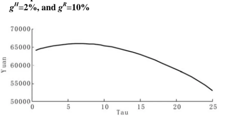
Figure 1 illustrates a similar situation. This plot essentially presents expanded data from the third data column of Panel B. The figure is a plot of
the net present benefit to the participant when τ is set equal to values of
between 0.5 years and 25 years, for gH=2% and gR=10%. Note that in this
case the net present value initially increases as τ increases and then in year 7
declines and declines every year thereafter. In this situation, the optimal
value of τ for the participant would be 7 years.
Figure 1: Net present benefit of HPF as a function of τ when T=25,
gH
=2%, and gR=10%
Other Parameter values: H0=175,000, M0=300; gM=3% , y0=12,000, gY=5%,
rS=4.5%, rf=6.5%, α=.33, R
0=1000, ξ=1, β=6%
One effect at first counter-intuitive is that when τ is equal to T, changing gR
does not affect the participant’s net present benefit. To understand this one must recall that net present benefit is the difference between the employee’s position if they rented and were not a participant in HPF minus their position
given that they are in HPF, as outlined in Eq. (9). If τ=T, the employee’s
in the rental growth rate do not affect the participant’s net present benefit.
The Effect of the Mortgage Subsidy and the Maintenance Growth Rate
A primary stated motivation for the privatization of public housing has been the rapid increase in government-born maintenance costs. This begs the question as to why an individual would be willing to take on these costs if the government finds them so onerous. One potential answer to that question is that it may be the case that an owner-occupant of the property can maintain the house more efficiently than can the government. Also, the physical deterioration of an owner occupied property tends to be much milder than a renter occupied property since the owner has an incentive not to abuse the property.
If maintenance costs significantly detract from the attractiveness of the program one option available to the government would be to provide an additional subsidy to the homeowner. This subsidy could either be direct or indirect. From the perspective of this model a direct subsidy would show up simply as a lower growth rate in maintenance costs. One way of providing an indirect subsidy would be to subsidize the mortgage rate. In fact, the mortgage rate is already subsidized, having averaged 4.5% over the past
several years when the risk free rate has been closer to 6.5%.30 A benefit of
subsidizing the mortgage rate – as opposed to other subsidies such as
increasing ξ– is that the subsidy would only start after the HPF participant
purchased their housing unit.
Table 6 examines how gM and rs affect the net present benefit of the HPF
participant for various combinations of T and τ. The table consists of Panels
A, B, and C. As in Tables 4 and 5 the panels correspond to different T values,
but in this case T takes on values of 10, 25, and 45 years, respectively.
Within each panel τ is set to a range of values from 0.5 years to the value of
T, gM is set to values of 2%, 6%, and 10%, and rs is set to values of 2.5%,
6.5%, and 10.5%. The values of rswere selected to correspond to three states:
a heavily subsidized rate (2.5%), a marginally subsidized rate (6.5%, which is the same as the risk-free rate), and a non-subsidized rate (10.5%).
While it is the case that increasing gM monotonically reduces the net present
benefit to the HPF participant, the magnitude of this reduction varies
depending upon the participant’s time horizon T and the expected time of
house purchase, τ. In Panel A, where T is set to 10 years, the effect of gM is
very small. In Panel C, where T is set to 45 years, when τ is 0.5 years the
effects of increasing gM are large. In the case where rs is 6.5%, increasing gM
from 2% to 10% reduces the net present benefit to the HPF participant by 27,046 Yuan, taking them from a positive net benefit of 3,351 Yuan to a
negative net benefit of –23,695 Yuan. If τ is set to 35 years, however, the
same change in gM results in only a decrease of only 21,728 Yuan in net
present benefit. The reason for this is, of course, that as τ increases, the
participant bears the maintenance cost for a shorter period of time.
Table 6: Net present benefit of HPF in Yuan for various values of T, τ, rs,
and gM
Other parameter values: y0=12,000 Yuan, gY=.05, rf=6.5%, H0=175,000, gH=2%, ξ=1.0, α=0.33,
M0=300, β=6%, R0=1000, gR=2% Panel A, T=10 years rs 2.5% 6.5% 10.5% gM gM gM τ 2% 6% 10% 2% 6% 10% 2% 6% 10% 0.5 82,902 82,393 81,729 67,097 66,588 65,923 51,291 50,782 50,118 5 81,349 80,977 80,469 74,659 74,287 73,779 67,970 67,597 67,089 10 81,448 81,448 81,448 81,448 81,448 81,448 81,448 81,448 81,448 Panel B, T=25 years rs 2.5% 6.5% 10.5% gM gM gM τ 2% 6% 10% 2% 6% 10% 2% 6% 10% 0.5 52,846 50,300 45,361 25,518 22,972 18,033 –1,809 –4,356 –9,294 5 50,620 48,210 43,428 33,081 30,672 25,889 15,542 13,133 8,350 10 48,858 46,820 42,546 39,870 37,832 33,558 30,882 28,844 24,570 25 53,076 53,076 53,076 53,076 53,076 53,076 53,076 53,076 53,076 Panel C, T=45 years rs 2.5% 6.5% 10.5% gM gM gM τ 2% 6% 10% 2% 6% 10% 2% 6% 10% 0.5 35,755 29,454 8,710 3,351 –2,950 –23,695 –29,054 –35,355 –56,099 5 33,232 27,068 6,480 10,319 4,749 –15,893 –11,405 –17,570 –38,158 10 30,650 24,858 4,778 17,702 11,910 -8,170 4,754 –1,038 –21,118 25 30,908 27,153 11,347 30,908 27,153 11,347 30,908 27,153 11,347 35 35,872 33,915 24,144 35,872 33,915 24,144 35,872 33,915 24,144 45 39,307 39,307 39,307 39,307 39,307 39,307 39,307 39,307 39,307
The mortgage rate, rs, also plays a major role in the value of the HPF
program to the participant. As in the case of gM, the magnitude of the effect
of rs on the net present benefit to the participant is a function of both T and τ.
For example, when rs is equal to 10.5%, increasing the participant’s time
horizon from 10 to 45 years, while holding τ constant at .5 years, and with
gM at only 2%, results in a decline of 80,285 Yuan, from 51,291 Yuan to
a large decline in the participant’s net benefit. One obvious reason is because
with the increased T value, the participant pays the mortgage rate for a
longer time, but it is also the case that with the longer time horizon the participant bears the maintenance cost for a longer time. If the mortgage rate
were subsidized, however, increasing T will still decrease the value of the
net present benefit, but it will be a significantly smaller amount. For example,
with rs at 2.5%, and with gM at 2%, the net present benefit declines by
27,456 Yuan – roughly one third of the decline when rs is set to 10.5%.
There are a couple of surprising results in Table 6 that deserve mentioning. The first is that when τ and T are set equal to each other neither gM nor rs
affect the participant’s net present benefit. As noted earlier, when τ and T are
equal the model assumes that the HPF participant purchases a