Wind Power Forecasting Pilot Project
Part B: The Quantitative Analysis
Final Report
A Report to: The Alberta Electric System Operator
2500, 330-5th Avenue SW
Calgary , Alberta
T2P 0L4
Attention: Mr. Darren McCrank, P.Eng.
Wind Power Forecasting Pilot Project
Project Manager
Fax: (403) 539-2949
Submitted by: Donald (Don) C. McKay, Ph.D., MBA
General Manager Tel: (905) 822-4120, Ext. 499 Fax: (905) 855-0406 E-mail: [email protected] Report No.: 70093-4 65 pages, 5 Appendices Date: August 18, 2008 www.ortech.ca
DISCLAIMER
The conclusions reached in this report were arrived at using data and other information provided to ORTECH by others. The activities of ORTECH in preparing this report were limited to analyzing the data and other information supplied to ORTECH. Except in the case of obvious anomalies or discrepancies no attempt was made to verify the data or the accuracy thereof as such activities were beyond the scope of ORTECH’s engagement. While ORTECH prepared this report in accordance with professional standards and has no reason to question the data or information provided to it, ORTECH assumes no responsibility or liability for the accuracy, completeness or veracity of the data or other information supplied to it in the course of preparing this report.
TABLE OF CONTENTS
Page No. EXECUTIVE SUMMARY ...1 1.0 INTRODUCTION ...7 2.0 DATA SETS ...9 2.1 Data Completeness...143.0 RESULTS AND ANALYSES...19
3.1 What is the General Accuracy of the Forecasts? ...21
3.1.1 MAE and RMSE Wind Speed ...21
3.1.1.1 Decomposition of RMSE ...26
3.1.2 RMSE and MAE Power...29
3.1.2.1 Normalized RMSE...31
3.1.2.2 Normalized MAE... 3.2 What is the accuracy of the Forecasts at the different forecast horizons studied (T=1 hour to T=48 hours)?...34
3.3 What is the accuracy of the Forecasts at different hours of the day and seasons of the year?...36
3.3.1 Hours of the Day...36
3.3.2 Seasons of the Year ...36
3.4 What is the accuracy of the Forecasted Meteorological Data before Running through the Power Conversion models? ...39
3.5 What is the accuracy of the Power Conversion? ...39
3.6 What is the Potential co-variance from given data samples? ...42
3.7 What is the accuracy of the Forecast at different wind speeds or different points of a Wind Power Facility’s power curve?...42
3.8 What is the relative comparison between Forecasts? ...46
3.8.1 Contemporary Analyses...46
3.8.1.1Wind ...46
3.8.1.2Power ...47
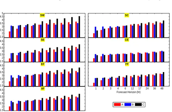
3.8.2 Performance Index...49
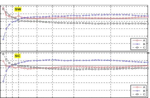
3.8.2.1Root Mean Square Error of Wind and Power Forecasts...49
3.8.2.2Bias of Wind and Power Forecasts...51
TABLE OF CONTENTS
Page No. 3.9 Which is the region with the least amount of error? Which
forecaster forecasts best in that regions and why?...54
3.10 What is the effect of spatial smoothing on forecast error? ...55
3.11 How well do the forecasts predict fast ramp up and ramp down times, Event analysis (CSI)?...57
3.12 What is the Impact on data availability?...59
3.13 Are there times (day/month/weather pattern) when there is more uncertainty in the forecasts than other times?) ...59
3.14 What is the relationship between the spread of the min/max and the forecast error? ...60
3.15 What is the correlation factor between all three forecasts? Is this related to the forecast error? ...61
3.16 Summary of Findings...61
4.0 GENERAL OBSERVATIONS AND RECOMMENDATIONS ...63
4.1 Data ...63
4.2 Trial Period ...64
4.3 Freezing the Models...65
4.4 Existing vs. Future Sites ...65
TABLE OF CONTENTS
Page No. TABLES
Table 2-1 Summary of the 10-Minute Measured Wind Speed Data Recovery Rates for each Site during the Q4 (February 1, 2008 0:00 UTC
- April 30, 2008 23:00 UTC) ...12 Table 2-2 Summary of the Hourly-Averaged Measured Wind Speed Data
Recovery Rates for each Site during Q4 (February 1, 2008 0:00
UTC - April 30, 2008 23:00 UTC) ...12 Table 2-3 Summary of the 10-Minute Measured/Calculated Power Data
Recovery Rates for each Site during Q4 (February 1, 2008 0:00
UTC – April 30, 2008 23:00 UTC)...13 Table 2-4 Summary of the Hourly-Averaged Measured/Calculated Power
Data Recovery Rates for each of the Sites during Q4 (February 1,
2008 0:00 UTC – April 30, 2008 23:00 UTC)...13 Table 2-5 Summary of Acceptable Ranges of Variables used by ORTECH to
Screen-Out Measured/Calculated and Forecasted Wind and Power
Data ...14 Table 2-6 Summary of the Annual Recovery Rates of Measured
Hourly-Averaged Wind-Speed and Measured/Calculated Power Data at the
Different Sites and Regions from May 1, 2007 to April 30, 2008 ...16 Table 2-7 Summary of the Annual Recovery Rates of Hourly-Averaged
Wind-Speed Data-Sets used in the Statistical Analyses at Each of the Selected Horizons and at the Different Regions from May 1,
2007 to April 30, 2008...17 Table 2-8 Summary of the Annual Recovery Rates of Hourly-Averaged
Power Data-Sets used in the Statistical Analyses at Each of the Selected-Horizons and at the Different Regions from May 1, 2007
TABLE OF CONTENTS
Page No. Table 3-1 General Accuracy for Power Forecasts for Each Forecaster on an
Annual Base ...35 Table 3-2 Annual Relative Standard Deviations of Measured Wind Speed
and Power in Different Regions...40 Table 3-3 Annual Ration of MAE and RMSE for Power Normalized by the
Measured Average Power to MAE and RMSE for Wind Speed
Normalized by the Measured Mean Wind Speed ...41 Table 3-4 Sum of various metrics for nine horizons for wind and power for
the South West and South Central regions for all three forecasters ...53 Table 3-5 Annual Summary of Rapid Ramp Events for specified Time
Horizons captured by Each Forecaster (% of total number of events) When Event is Forecasted Not More Than 12 Hours In
advance of the Actual Event ...58 Table 3-6 Annual Summary of Rapid Ramp Events for Specified Time
Horizons Captured by Each Forecaster (% of total number of events) When Event is Forecasted Either 6 Hours Before or 6 Hours After the Actual Event ...58 Table 3-7 Confidence limits (%) of minimum and maximum predicted power
TABLE OF CONTENTS
Page No. FIGURES
Figure 3-1 Comparison of the time series of measured and predicted wind speeds at first forecast horizon (T=1hr) by an anonymous forecaster at a particular wind farm (name is not disclosed). Note
examples are circled...23 Figure 3-2 Annual Mean Absolute Error (MAE) of wind speed (WS)
predictions (Pred) in South West (SW), South Central (SC), South East (SE), Central (CE), Existing Facilities (EF), Future Facilities (FF) and All Facilities (AF) by three forecasters A, B and C as a
function of forecast horizons. ...24 Figure 3-3 Annual Root Mean Square Error (RMSE) of wind speed (WS)
predictions (Pred.) in South West (SW), South Central (SC), South East (SE), Central (CE), Existing Facilities (EF), Future Facilities (FF) and All facilities (AF) by three forecasters A, B and C as a
function of forecast horizons. ...25 Figure 3-4 Annual errors of wind speed predictions in South West (SW),
South Central (SC), South East (SE), Central (CE), Existing Facilities (EF), Future Facilities (FF) and All Facilities (AF) by Forecasters A, B, and C as a function of forecast horizon. Note that RMSE and its components: dispersion (disp), bias (bias) and standard deviation of bias (sdbias) are shown with different symbols and colors...28 Figure 3-5 Annual Normalized Root Mean Square Error (RMSE %) of Power
predictions in South West (SW), South Central (SC), and existing facilities (EF) by three forecasters A, B and C as a function of forecast horizons. Note that the actual errors are normalized by the
rated capacity (RC) of the region of power aggregation ...30 Figure 3-6 Annual Errors of power predictions in South West (SW), South
Central (SC), Existing Facilities (EF), by Forecasters A, B, and C as a function of forecast horizon. Note that RMSE and its components: dispersion (disp), bias (bias) and standard deviation
TABLE OF CONTENTS
Page No. Figure 3-7 Normalized Root Mean Square Error (RMSE) of Power
predictions in South West (SW), South Central (SC), and existing facilities (EF) by three forecasters A, B and C as a function of forecast horizons. Note that the actual errors are normalized by the
rated capacity of the region of power aggregation. ...33 Figure 3-8 Accuracy of the Power Forecast for Specific 6 Hour Time Periods
for Each Forecaster Using RMSE (% Rated Capacity for the South
West (SW), South Central (SC), and Existing Facilities (EF)...37 Figure 3-9 Seasonal Accuracy of the Power Forecast for Each Forecaster
Using RMSE (% Rated Capacity) for the South West (SW), South
Central (SC), and Existing Facilities (EF)...38 Figure 3-10 Typical Power Curve (GE 1.5 MW sle)...42 Figure 3-11 Annual RMSE of wind speed predictions at the chosen forecast
horizons (T = 1, T =2 and T = 48hr) in Existing Facilities (EF) by
Forecasters A, B and C as a function of predicted wind speed ...44 Figure 3-12 Annual Normalized RMSE of Power for Existing Facilities at
Different Predicted Wind Speed Bins...45 Figure 3-13 RMSE Annual Comparison between Forecasters for Wind by
Region...47 Figure 3-14 Annual Comparison between Forecasters for Power by Region
(Normalized RMSE % of Rated Capacity (RC)) and a Comparison
against Persistence for SW, SC Regions and EF. ...48 Figure 3-15 Annual Comparison between Forecasters Against Persistence for
SW, SC Regions and EF for Power using SS (RMSE)...48 Figure 3-16 Annual Normalized Performance Index for Wind using RMSE for
Four Regions for the Three Forecasters...50 Figure 3-17 Annual Normalized Performance Index for Power Using RMSE in
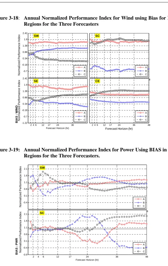
Two Regions for the Three Forecasters...50 Figure 3-18 Annual Normalized Performance Index for Wind using Bias for
Four Regions for the Three Forecasters...52 Figure 3-19 Annual Normalized Performance Index for Power Using Bias in
TABLE OF CONTENTS
Page No. Figure 3-20 Annual Ratio of Regional Standard Deviation of Power Prediction
Errors to the Average Standard Deviation of the Individual Sites in
the Region for Various Region Sizes and Forecast Horizons...56 APPENDICES
Appendix A Alberta Forecast Regions Appendix B Bibliography
Appendix C Data Completeness for Each Quarter Appendix D Selected Wind Statistics by Quarter Appendix E Selected Power Statistics by Quarter
EXECUTIVE SUMMARY
As part of the Alberta Energy System Operator’s (AESO) wind power forecasting pilot project, ORTECH Power (ORTECH) was contracted to provide quantitative analysis services. Wind and power forecast data was provided by three independent wind forecasting firms, referred to herein as Forecaster A, Forecaster B and Forecaster C. The analysis consisted of comparing the predicted data against measured meteorological power data for seven existing Alberta wind power facilities (Existing Facilities), and measured meteorological data and derived power data for five future Alberta wind power facilities (Future Facilities). The measured, predicted, and simulated data was collected and distributed to the forecasters and ORTECH by GENIVAR (Phoenix Engineering). Analysis was carried out by examining the available data from each of the forecasters in seven categories, consisting of the entire dataset All Facilities (AF), Existing Facilities (EF), Future Facilities (FF), and four geographic regions. To define the four regions, the available data for the Existing Facilities and the Future Facilities were distributed geographically into South West (SW) Region, South Central (SC) Region, South East (SE) Region, and a Central Region (CE) (see map in Appendix A). The analysis for the individual facilities was not included in this report due to confidentially requirements.
The forecast data was analyzed using statistical methods with an emphasis on deriving meaningful and precise values for averaged errors between predicted and observed data that would provide some insight into the error characteristics based on the diagram below.
Observations: Hourly time-scale
Forecasts: 1 to 48 hour time scales
Meteorological situations: 3 to >8 hour time scales
Temporal statistics: 1 to 48 hour time horizons
and Seasonal
Stratified Statistics: season and meteorological
situation Summary statistics: confidence intervals etc. resolved 1 to 48 hour horizons Distinction between forecasters: resolved 1 to 48 hour horizons
The final report documents the analysis for the one-year study period, extending from May 1, 2007 to April 30, 2008, inclusive.
The final report attempts to draw out specific findings and/or insights based on a set of questions posed by the working group after reviewing the three progress reports. The questions posed by the working group were;
1. What is the general accuracy of the Forecasts?
2. What is the accuracy of the Forecasts at the different forecast horizons studied (T=1 hour to T=48 hours)?
3. What is the accuracy of the Forecasts at different hours of the day and seasons of the year?
4. What is the accuracy of the Forecasted Meteorological Data before running through the Power Conversion models?
5. What is the accuracy of the Power Conversion?
6. What is the Potential co-variance from given data samples?
7. What is the accuracy of the Forecast at different wind speeds or different points of a Wind Power Facility's power curve?
8. What is the relative comparison between Forecasts?
9. Which is the region with the least amount of error? Which forecaster forecasts best in that region and why?
10.What is the effect of spatial smoothing on forecast error?
11.How well do the forecasts predict fast ramp up and ramp down times, event analysis (CSI)?
12.What is the Impact on data availability?
13.Are there times (day/month/weather pattern) when there is more uncertainty in the forecasts than other times?
14.What is the relationship between the spread of the min/max and the forecast error?
15.What is the correlation factor between all three forecasts? Is this related to the forecast error?
The report is presented as follows:
Section 2.0 – describes the data sets provided by GENIVAR (Phoenix
Engineering)
Section 3.0 – the results and analyses (response to questions posed by working
group)
Section 4.0 – general observations and recommendations
From the analyses undertaken in Section 3.0, addressing questions raised by the working group, a summary of the findings was produced which is outlined below. After each finding the relevant section were the analysis is discussed is indicated. The summary of findings is;
1. Forecasting wind energy in the regions examined in Alberta over a 48 hour time horizon is possible (all sections)
2. All three forecasters can provide general forecasts in the regions examined over the 48 hour time horizon.(sections 3.1 and 3.8)
3. The largest error in the forecasts is due to phases errors. The different regions show a consistent behaviour for phase error suggesting a similar property affects all regions in a similar manner. (sections 3.1 and 3.2) 4. The accuracy of the forecasts in general decreases as the forecast horizon
increases. While there is a variation between forecasters in accuracy at each forecast horizon, the trend of decreasing accuracy as the forecast horizon increases is preserved by each forecaster. (sections 3.1 and 3.2) 5. The wind power forecasts are the least accurate during the afternoon
periods between hours 13 and 18 after forecast horizon T=6. (section 3.3) 6. The least accurate wind power forecasts are during the winter season
(November, December, January, February) for all forecasters. The best accuracy is during the summer season (June, July, and August). (section 3.3)
7. Wind speed prediction errors are amplified by 1.0 – 1.5 due to power conversion. (section 3.5)
8. The power prediction errors peak at the predicted wind speed of 10 m/s and show a different pattern from the wind speed error.(section 3.7) 9. The region with the least amount of error for wind is the central region
(CE). The region with the largest amount of error is the Southwest Region (SW). (section 3.9)
10. For power forecasts, the accuracy for both SW and SC regions are similar. (section3.9)
11. Spatial smoothing reduces the error as the number of wind farms and the size of the area covered increases. (section 3.10)
12. All forecasters do not predict ramp events effectively. The reason may be that the forecasters were not given this specific objective. (section 3.11) 13. In examining the min-max spread for predicted power it was found that
the measured values fell between the min-max predicted power 81%-95% of the time. (section 3.14)
A number of general observations and recommendations are presented. These include:
a) Data
(i) ORTECH relied on GENIVAR (Phoenix Engineering) for providing a QA/QC’d measured data-sets for the different sites. Although, ORTECH applied a screen out criteria on the data, more confidence could have been achieved if one or both of the recommendations listed below was employed:
• Recommendation 1: GENIVAR (Phoenix Engineering) to provide
ORTECH with a coded data-set along with a key to the codes used to substitute invalid data based on their QA/QC procedures. A detailed QA/QC report would also be helpful
• Recommendation 2: ORTECH to receive a raw database and to apply
its own QA/QC measures which include the following:
» Reviewing instruments orientation and calibration reports and correcting the data accordingly when necessary.
» Flagging data with abnormal wind speeds or power and/or standard deviations and filtering them out if they fall outside of a certain or agreed-upon range.
» Screening the data for icing events or any other anomalies that may have not been caught in the screening-out criteria and filtering them out.
» Comparing wind speed data from different anemometers levels and from adjacent sites looking for discrepancies that are then filtered when necessary.
» Other site specific QA/QC procedures.
(ii) Some of the measured-data were modified and/or added after the end of each quarter. It was expected to have the data QA/QC’d and ready to be analyzed before they were posted on GENIVAR’s (Phoenix Engineering) wind-server for ORTECH to download, which was not the case.
• Recommendation: ORTECH to receive final and unchanged values in
(iii) ORTECH had neither access to the measured data provided to each of the forecasters nor to their availability. It was assumed that the measured data made available to ORTECH and to each of the forecasters were comparable.
• Recommendation: ORTECH to receive a data-availability report from
each of the forecasters summarizing the hours that were used from the measured data to produce their forecast. A more reliable comparison between the different forecasters could have been produced.
(iv) ORTECH assumed that none of the forecasters did prescreening to their results. The fact that in some cases forecasters did not provide forecasts up to the 48th time horizon (T=48) puts this assumption into question.
• Recommendation: ORTECH to receive from each of the forecaster
reports summarizing their prescreening criteria and listing their omitted forecasts if they do prescreening or a statement saying that they do not.
b) Trial Period
In undertaking such a large project a trial period would have been advantageous. This trial period would allow all the components of the project (forecasters, data providers, data analyst) to test their procedures to ensure that the logistics were running as smoothly as possible. It is recommended that at least a two to three month trial period be undertaken before the main project is initiated. The trial period could be undertaken using a subset of the sites.
c) Freezing the Models
Provided one of the questions to be addressed is a comparison between forecasters then it is recommended that after an initial training period the forecast model codes be frozen. If they are not frozen the consultant doing the quantitative analysis can not predict whether the output at the start of the project was the same as the output generated from the forecast model at the end of the project. Another alternative would be to have each forecaster describe in detail the changes made to the model as the project progressed.
d) Existing vs. Future Sites
Given, that the main emphasis of the study was on wind power forecasting and not wind speed forecasting, it is recommended, that only existing sites which have measured wind power data be used. By using only measured wind power data a more representative indication of the accuracy of the forecaster’s power conversion methodologies is provided.
e) Focusing on the Priorities
Given the amount of data, the presentation and analysis of the information generated was considerable. It is recommended that future Working Groups in cooperation with the consultants determine what are the specific questions that are to be addressed and thus defining the metrics/analyses that will be the focus of the progress and final reports.
1.0 INTRODUCTION
As part of the Alberta Energy System Operator’s (AESO) wind power forecasting pilot project, ORTECH Power (ORTECH) was contracted to provide quantitative analysis services. Wind and power forecast data was provided by three independent wind forecasting firms, referred to herein as Forecaster A, Forecaster B and Forecaster C. The analysis consisted of comparing the predicted data against actual meteorological data and real power data for seven existing Alberta wind power facilities and actual meteorological data and derived power data for five future Alberta wind power facilities.
Analysis was carried out by examining the available data from each of the forecasters in seven categories, consisting of the entire dataset All Facilities (AF), Existing Facilities (EF), Future Facilities (FF) and four geographic regions. To define the four regions, the available data for the Existing Facilities and the Future Facilities were distributed geographically into South West (SW) Region, South Central (SC) Region, South East (SE) Region, and a Central Region (CE) (see map in Appendix C). The analysis for the individual facilities was not included in this report due to confidentiality concerns. AESO and the forecasters have access to all the graphs produced using their datasets which were provided to ORTECH for the purposes of this final report prior to issuing it.
This report documents the analysis for the one-year study period, extending from May 1, 2007 to April 30, 2008, inclusive.
The final report deviates from the three quarterly progress reports provided previously in that the final report attempts to emphasize more insight into what the information is saying as opposed to just providing the metrics. As well, the report attempts to address the questions posed by the working group, derived after reviewing the three quarterly reports. The questions posed by the working group are as follows;
1. What is the general accuracy of the Forecasts?
2. What is the accuracy of the Forecasts at the different forecast horizons studied (T=1 hour to T=48 hours)?
3. What is the accuracy of the Forecasts at different hours of the day and seasons of the year?
4. What is the accuracy of the Forecasted Meteorological Data before running through the Power Conversion models?
6. What is the Potential co-variance from given data samples?
7. What is the accuracy of the Forecast at different wind speeds or different points of a Wind Power Facility's power curve?
8. What is the relative comparison between Forecasts?
9. Which is the region with the least amount of error? Which forecaster forecasts best in that region and why?
10. What is the effect of spatial smoothing on forecast error?
11. How well do the forecasts predict fast ramp up and ramp down times, event analysis (CSI)?
12. What is the Impact on data availability?
13. Are there times (day/month/weather pattern) when there is more uncertainty in the forecasts than other times?
14. What is the relationship between the spread of the min/max and the forecast error?
15. What is the correlation factor between all three forecasts? Is this related to the forecast error?
Figures and tables are presented in the report proper as an illustration of the data used in support of addressing the questions. The complete set of figures and tables used to address each question are presented on a CD accompanying this report due to the large amount of information
Only power data from the Existing Facilities and the two regions (SW,SC) which only have existing facilities are presented since for the Future Facilities one can not compare predicted power against a measured power.
For completeness, selected tables and figures for wind speed and power by quarter are presented in Appendix C to E.
The report is presented as follows:
Section 2.0 – describes the data sets provided by GENIVAR (Phoenix
Engineering)
Section 3.0 – the results and analyses (response to questions posed by working
group)
2.0 DATA
SETS
GENIVAR (Phoenix Engineering) made the following data available and accessible to ORTECH:
a) Actual meteorological data and real power data for seven (7) existing Alberta wind power facilities and actual meteorological data and calculated wind power data from five (5) future Alberta wind power facilities from May 1, 2007 to April 30, 2008, inclusive.
b) Forecast meteorological and power datasets for seven (7) existing Alberta wind power facilities, five (5) future facilities and the different Regions (i.e. South West (SW), South Central (SC), South East (SE), Central (CE), Existing-Facilities (EF), Future-Facilities (FF) and All-Facilities (AF)) from three (3) forecasters for May 1, 2007 to April 30, 2008, inclusive, every hour, on the hour.
Both actual and forecasted data gathered for the first, second and third quarter progress reports (i.e. Q1, Q2 and Q3) were used in this final report to cover for May 1, 2007 to July 31, 2007, August 1, 2007 to October 31, 2007 and November 1, 2007 to January 31, 2008 periods respectively. To complete a full year, ORTECH collected a fourth quarter dataset (February 1, 2008 to April 30, 2008) from GENIVAR (Phoenix Engineering) in the same fashion as the other quarters. Changes to the data made available by GENIVAR (Phoenix Engineering) after the end of each quarter were not incorporated into the datasets used by ORTECH. Also power data forecasts for “Existing-Facilities (EF)” (the Region) were evaluated based on eleven rather than twelve months of data from June 2007 to April 2008 since forecasted power datasets for the month of May 2007 for “Existing-Facilities (EF)” for all forecasters were not complete.
ORTECH relied solely on the aforementioned data-source and monitored the source to ensure all the data and/or information considered necessary for performing this analyses was available.
The measured meteorological data i.e. wind speeds at different heights, wind direction, barometric pressure and temperature at each individual site (a total of 12 sites) were retrieved from GENIVAR (Phoenix Engineering) historical-readings wind server. The naming convention was provided by AESO and the output attained is the ten (10) minute average data which was then averaged on an hourly basis by ORTECH. Only the hours with an acceptable count (≥ 80%) of valid ten (10) minute data were taken into consideration. ORTECH has also converted the time stamps of the retrieved data from Mountain Standard Time (MST) to Universal Time (UTC) in order to perform the analyses against the forecasted data; hence, ascertaining an “apple to apple” comparison.
The measured power data at the existing facilities were also acquired from GENIVAR (Phoenix Engineering) historical-readings wind server in the same manner as the meteorological data except for a different naming convention; “AESO.CSDR2” which stands for AESO Current Supply and Demand. Power data were obtained at the seven (7) existing facilities for the months of February, March and April (for the 4th quarter). The predicted/calculated power data for the five (5) future sites were provided to ORTECH by GENIVAR (Phoenix Engineering) through their ftp site.
Transmission constraint periods for each month at specific sites were provided to ORTECH by AESO. ORTECH applies a “-997” code to the data during these periods which are then rejected when applying a screen-out criteria based on acceptable ranges listed in Table 2-5 in section 2.1.
Similar to previous quarters, each of the three (3) forecasters has provided forecast datasets for each of the twelve (12) sites as well as the four (4) regions (i.e. South-West (SW), South-Central (SC), South-East (SE) and Central (CE)) and for Existing-Facilities (EF), Future-Facilities (FF) and All-Facilities (AF). These datasets were made available to ORTECH through GENIVAR (Phoenix Engineering) website for the 4th quarter as well; February 1, 2008 to April 30, 2008, inclusive, every hour, on the hour. Each dataset consists of a forecast for forty-eight (48) forecast time horizons: T=1 (one hour ahead) to T=48 (48 hours ahead) and they are divided into two categories: meteorological and power. The meteorological datasets include forecasted wind speed, wind direction, temperature, air pressure and their uncertainty (min/max) and averages at each of the twelve (12) sites. The power datasets include forecasted power and ramp rate and their uncertainty (min/max) at each of the twelve (12) sites and the aforementioned four regions and EF, FF and AF.
Tables 2-1 to 2-4 provide the monthly and total 10-minute and hourly averaged measured wind speed and measured/calculated power data recovery rates (prior to employing the screen-out criteria detailed in section 2.1) for the 4th quarter (Q4) from February 1, 2008 to April 30, 2008, respectively. Similar tables for the 1st quarter (Q1), 2nd quarter (Q2) and 3rd quarter (Q3) are shown in Appendix C. The data recovery rate is defined as the number of valid data records collected versus that possible over the reporting period. The method of calculation is as follows: (100) * Possible Records Data Collected Records Data (%) Rate Recovery Data = Where,
Data Records Collected = Data Records Possible – Number of Invalid Records As shown in Tables 2-1 and 2-2 the 10-minute and hourly recovery rate for the measured wind speed during the 4th quarter were generally ≥ 97% except for site 8 and site 10 which, returned a 10-minute recovery rate of 81.2%.and 87.3%, respectively. The low recovery rate at site 8 has resulted from a SCADA PC/hardware problem detected during the month of February; hence, returning a recovery rate as low as 52.3% for that month.
The recovery rate for the power data were also reasonable (≥ 98%) throughout the analysis period of the 4th quarter as shown in Tables 2.3 and 2.4.
A 90% overall recovery rate is normally considered as the minimum requirement by the industry to be temporally representative.
Table 2-1: Summary of the 10-Minute Measured Wind Speed Data Recovery Rates for each Site during Q4 (February 1, 2008 0:00 UTC – April 30, 2008 23:00 UTC)
10 Minute Data Recovery Rate (%)
Site/Month February March April All Months
1 99.0 99.8 99.2 99.3 2 94.8 100.0 99.4 98.1 3 99.7 99.7 98.9 99.5 4 99.7 100.0 98.9 99.5 5 99.7 99.9 99.2 99.6 6 99.8 99.1 93.0 97.3 7 99.3 100.0 99.2 99.5 8 52.3 93.9 97.3 81.2 9 98.0 99.7 99.2 98.9 10 62.0 100.0 100.0 87.3 11 99.9 100.0 99.9 99.9 12 100.0 100.0 100.0 100.0
Table 2-2: Summary of the Hourly-Averaged Measured Wind Speed Data Recovery Rates for each Site during Q4 (February 1, 2008 0:00 UTC – April 30, 2008 23:00 UTC)
Hourly Data Recovery Rate (%)
Site/Month February March April All Months
1 99.0 100.0 99.0 99.3 2 94.0 100.0 99.0 97.7 3 100.0 100.0 99.0 99.7 4 100.0 100.0 99.0 99.7 5 99.0 100.0 99.0 99.3 6 100.0 99.0 92.0 97.0 7 99.0 100.0 99.0 99.3 8 52.0 94.0 97.0 81.0 9 98.0 100.0 99.0 99.0 10 62.0 100.0 100.0 87.3 11 100.0 100.0 100.0 100.0 12 100.0 100.0 100.0 100.0
Table 2-3: Summary of the 10-Minute Measured/Calculated Power Data Recovery Rates for each Site during Q4 (February 1, 2008 0:00 UTC – April 30, 2008 23:00 UTC)
10-Minute Data Recovery Rate (%)
Site/Month February March April All Months
1 100.0 100.0 100.0 100.0 2 98.5 100.0 100.0 99.5 3 100.0 100.0 100.0 100.0 4 100.0 100.0 100.0 100.0 5 100.0 100.0 100.0 100.0 6 100.0 100.0 100.0 100.0 7 98.3 99.9 97.7 98.6 8 100.0 99.7 99.9 99.9 9 97.0 99.7 97.6 98.1 10 98.6 99.8 97.5 98.6 11 98.6 99.8 97.5 98.6 12 98.7 99.9 97.5 98.7
Table 2-4: Summary of the Hourly-Averaged Measured/Calculated Power Data Recovery Rates for each of the Sites during Q4 (February 1, 2008 0:00 UTC – April 30, 2008 23:00 UTC)
Hourly Data Recovery Rate (%)
Site/Month February March April All Months
1 100.0 100.0 100.0 100.0 2 98.4 100.0 100.0 99.5 3 100.0 100.0 100.0 100.0 4 100.0 100.0 100.0 100.0 5 100.0 100.0 100.0 100.0 6 100.0 100.0 100.0 100.0 7 98.0 99.9 97.8 98.6 8 100.0 100.0 99.9 100.0 9 96.6 99.7 97.8 98.0 10 98.4 99.7 97.8 98.6 11 98.4 99.7 97.8 98.6 12 98.4 99.9 97.6 98.6
2.1 Data Completeness
ORTECH did not apply a “standard” quality control and quality assurance procedures on the measured or forecasted data retrieved. Instead, screen-out criteria is; however, employed on both datasets following a list of acceptable ranges, approved by AESO, for the different variables as detailed in Table 2-5. Values laying outside of these ranges were rejected.
In order to perform legitimate statistical analyses, a “complete” set of data is required. Therefore, ORTECH in the analyses of the four quarters considered only data-sets that are valid (based on the screen-out criteria) and available from all sources (i.e. measured and forecasted from forecasters A, B and C). If data are invalid or missing at a specific hour/period from one of the aforementioned sources, ORTECH rejects that hour/period and does not consider them in the statistical analyses.
Table 2-5: Summary of Acceptable Ranges of Variables used by
ORTECH to Screen-Out Measured/Calculated and Forecasted Wind and Power Data
Variable Acceptable Range (inclusive)
Wind Speed (m/s) 0 to 60
Wind Direction (°) 0 to 360
Power (MW) -0.1 x site-specific rated capacity to 1.1 x site-specific rated capacity
Surface Temperature (°C) -60 to 60
Surface Pressure (mbar) 500 to 1500
The annual recovery rate for the hourly-averaged measured wind-speed and measured/calculated power after applying the screen-out criteria for the reporting period (May 1, 2007 to April 30, 2008) are summarized in Table 2-6. Each of the four (4) regions (SW, SC, SE and CE) includes three existing and/or future wind farms; thus, ORTECH has stacked together the wind speed data from the sites relevant for each region since it is difficult to generalize and/or normalize the wind speed for each Region. The wind speed recovery rates calculated for those Regions and presented in Table 2-6 are; subsequently, calculated based on the stacked data; hence, one should be careful before drawing any conclusions based on these recovery rates.
The annual recovery rate (R) for wind-speed and power “complete” data-sets that are used in the statistical analyses at each of the Selected-Horizons and at the different Regions are summarized in Tables 2-7 and 2-8 respectively and they are calculated as follows:
R = Number of hours with available and valid data during the year of analysis Number of hours possible during the year of analysis (i.e. 8784 hours) The annual average recovery rates for the “complete” data-set of hourly-averaged wind-speed were greater than 90% in all Regions except for the CE and FF where the annual average recovery rates returned were 83.6% and 87.2%, respectively as shown in Table 2-7. These rather low recovery rates are the result of the low recovery rates (illustrated in Table 2-6) returned for the measured wind-speed at some of the future sites particularly sites 10, 11 and 12 which fall within those regions.
The annual recovery rates for the “complete” data-set of power were greater than 92% for the SW, SC and CE regions while they were around 90% for the SE, CE and EF with the lowest for the latter region which returned an annual recovery rate of 88.1% as illustrated in Table 2-8. The fairly low annual recovery rate at this region (i.e. EF) has resulted from incomplete forecasted power data (from all forecasters) during the month of May 2007. To avoid misleading results ORTECH considered only eleven months (11) from June 2007 to April 2008, inclusive for the existing-facilities in the analyses of power (summarized in the following sections).
Table 2-6: Summary of the Annual Recovery Rates of Measured Hourly-Averaged Wind-Speed and Measured/Calculated Power Data at the Different Sites and Regions from May 1, 2007 to April 30, 2008
Site/Region
Recovery Rate of Hourly Wind Speed Data
(%)
Recovery Rate of Hourly Power Data (%) 1 97.9 99.5 2 90.1 97.6 3 98.9 99.9 4 97.6 99.4 5 94.9 99.5 6 97.7 99.7 7 94.2 94.1 8 89.3 99.4 9 96.2 95.3 10 82.9 98.4 11 86.1 98.0 12 88.0 98.3 SW 95.6 97.5 SC 93.9 99.2 SE 96.0 92.7 CE 85.7 97.5 EF 95.2 97.0 FF 89.5 92.8 AF 92.8 90.2
Table 2-7: Summary of the Annual Recovery Rates of Hourly-Averaged Wind-Speed Data-Sets used in the Statistical Analyses at Each of the Selected-Horizons and at the Different Regions from May 1, 2007 to April 30, 2008.
Data Recovery Rate (%) Horizon/Region SW SC SE CE EF FF AF T=1 93.8 92.2 94.0 84.0 93.4 87.6 91.0 T=2 93.8 92.2 94.0 84.0 93.4 87.6 91.0 T=3 93.8 92.2 94.0 84.0 93.4 87.6 91.0 T=4 93.8 92.2 94.0 83.9 93.4 87.6 91.0 T=6 93.8 92.2 93.9 83.9 93.4 87.6 91.0 T=12 93.7 92.1 93.8 83.9 93.3 87.5 90.9 T=17 93.7 92.0 93.7 83.8 93.2 87.4 90.8 T=24 93.5 91.8 93.6 83.7 93.1 87.3 90.6 T=36 93.3 91.6 93.3 83.4 92.8 87.0 90.4 T=48 92.3 90.7 92.5 82.6 91.9 86.2 89.5 Avg (T=1 -T=48) 93.4 91.7 93.5 83.6 93.0 87.2 90.6 Min (T=1 -T=48) 92.3 90.7 92.5 82.6 91.9 86.2 89.5 Max (T=1 -T=48) 93.8 92.2 94.0 84.0 93.4 87.6 91.0
Table 2-8: Summary of the Annual Recovery Rates of Hourly-Averaged Power Data-Sets used in the Statistical Analyses at Each of the Selected-Horizons and at the Different Regions from May 1, 2007 to April 30, 2008
Data Recovery Rate (%) Horizon/Region SW SC SE CE EF FF AF T=1 93.1 97.2 90.7 94.8 88.6 90.4 87.2 T=2 93.1 97.2 90.6 94.8 88.6 90.5 87.2 T=3 93.0 97.1 90.6 94.8 88.5 90.5 87.1 T=4 93.0 97.1 90.6 94.8 88.5 90.4 87.1 T=6 92.9 97.0 90.5 94.8 88.4 90.4 87.0 T=12 92.9 96.9 90.3 94.7 88.3 90.3 86.9 T=17 92.8 96.8 90.1 94.7 88.3 90.1 86.8 T=24 92.6 96.6 89.9 94.7 88.2 90.0 86.7 T=36 92.6 96.3 89.6 94.3 87.9 89.6 86.5 T=48 91.7 95.3 88.5 93.3 87.1 88.4 85.5 Avg (T=1 -T=48) 92.7 96.5 89.9 94.5 88.1 89.8 86.7 Min (T=1 -T=48) 91.7 95.3 88.5 93.3 87.1 88.4 85.5 Max (T=1 -T=48) 93.1 97.2 90.7 94.8 88.6 90.5 87.2
3.0
RESULTS AND ANALYSES
The forecast data was analyzed using statistical methods described in the first, second, and third quarterly reports. Emphasis was placed on deriving meaningful and precise values for a metric that characterizes the typical magnitude of error over all hours in the evaluation between the predicted and measured data. Most error measures produce numbers that assess the deviations between predicted and measured values, but it is more meaningful to arrive at a statement such as “at site
X, y% of the forecasts are within z value from the mean” which requires the
correct choice of error measure and some indication of the type of distribution. To this end, only those statistical parameters that provide some insight into the error characteristics are presented based on the diagram below.
Observations: Hourly time-scale
Forecasts: 1 to 48 hour time scales
Meteorological situations: 3 to >8 hour time scales
Temporal statistics: 1 to 48 hour time horizons
and Seasonal
Stratified Statistics: season and meteorological
situation Summary statistics: confidence intervals etc. resolved 1 to 48 hour horizons Distinction between forecasters: resolved 1 to 48 hour horizons
The final outcome should attempt to distinguish one forecast methodology from another resolved to 1 to 48 hour forecast horizons for various regions. The information provided in this report works toward that goal.
After reviewing the three quarterly reports the working group provided a set of specific questions that they wished to have addressed in the final report. The questions listed below are addressed in this section of the final report. In addressing these questions an extensive amount of statistical analysis was undertaken to try to provide some insight and support for any findings. At the direction of the working group the emphasis was put on power as opposed to wind. In some of the sections below metrics for both wind and power are presented. However following the working group’s direction most sections only show metrics for power. Similarly in most sections only one metric is shown which, is the Root Mean Square Error (RMSE). All the metrics, figures and tables used in the analysis are attached at the back of the report on a CD.
The questions that are addressed, as provided by the working group are as follows;
1. What is the general accuracy of the Forecasts?
2. What is the accuracy of the Forecasts at the different forecast horizons studied (T=1 hour to T=48 hours)?
3. What is the accuracy of the Forecasts at different hours of the day and seasons of the year?
4. What is the accuracy of the Forecasted Meteorological Data before running through the Power Conversion models?
5. What is the accuracy of the Power Conversion?
6. What is the Potential co-variance from given data samples?
7. What is the accuracy of the Forecast at different wind speeds or different points of a Wind Power Facility's power curve?
8. What is the relative comparison between Forecasts?
9. Which is the region with the least amount of error? Which forecaster forecasts best in that region and why?
10.What is the effect of spatial smoothing on forecast error?
11.How well do the forecasts predict fast ramp up and ramp down times, event analysis (CSI)?
12.What is the Impact on data availability?
13.Are there times (day/month/weather pattern) when there is more uncertainty in the forecasts than other times?
14.What is the relationship between the spread of the min/max and the forecast error?
15.What is the correlation factor between all three forecasts? Is this related to the forecast error?
Results are presented for the four (4) geographical regions: South-West (SW), South-Central (SC), South East (SE) and Central (CE), as well as, for Existing Facilities (EF), Future Facilities (FF) and All Facilities (AF) when wind speed is presented. When power is presented only the SW, SC and EF are presented in order to compare forecasted power to measured power.
Wind speed and power forecasts were provided each hour for forty-eight (48) hourly forecast horizons, T=1 (one hour ahead) to T=48 (48 hours ahead). In the following text “Selected Forecast Horizons” refers to T=1, T=2, T=3, T=4, T=6, T=12, T=17, T=24, T=36 and T=48 which were defined by the working group. As indicated in section 2.0, the forecasted power data-set for the month of May 2007 for Existing Facilities for all forecasters was not complete. Therefore, when evaluating the metrics for power for Existing Facilities only eleven months of data was used (June 2007-April 2008).
The results include those illustrations that were deemed relevant as mentioned above. A large number of additional illustrations can be generated from the statistical analysis, but were not included for practical reasons. They are available in the CD accompanying the report.
3.1 What is the General Accuracy of the Forecasts?
3.1.1 MAE and RMSE Wind Speed
Each of the four regions (SW, SC, SE, and CE) includes three existing or/and future facilities, thus it is difficult to generalize and/or normalize the wind speed for each region. Therefore, the assessment of the forecast errors for the wind speed was processed for each region without normalization, i.e., the predicted and measured pairs at those individual sites were simply stacked together for the relevant regions. What is meant by stacking, is grouping the wind data collected from sites at a particular region thereby considering them as one “long” data set. The objective of such a grouping is to derive regional error statistics for wind data without doing any averaging. The procedure of such grouping can be explained through an example as follows.
The South West region contains three meteorological masts. Therefore, three sets of wind data time series are available. These three data sets are combined together irrespectively (of dates/times). The error statistics are then calculated using the same method as for an individual site. With this approach averaged wind speed data from any individual time series are not derived.
In looking at the general accuracy of the wind speed as predicted by the forecasters in all regions and at all time horizons the Mean Absolute Error (MAE) and the Root Mean Square Error (RMSE) were the specific metrics used. In the case of the RMSE it was decomposed into its component part the bias and the variance of the error.
The RMSE connects the important statistical quantities of the two time series. It is composed of three different components which contribute to the RMSE originating from different effects. The bias accounts for the difference between the mean values of forecast and measurement. The standard deviation (sde)
measures the fluctuations of the error around its mean. The sde is very useful as it
directly provides the 68%-confidence interval if the errors are normally distributed.
In the context of comparing forecast and measurement, the sde has two
contributions. The first is the sdbias, i.e. the difference between the standard
deviations of predicted and measured values, which evaluates errors due to wrongly forecasted variability. This together with the bias is an indicator of
amplitude errors. The second contribution is the dispersion (disp) which involves
the cross-correlation coefficient (r) weighted with the standard deviations of both
time series. Thus, disp accounts for the contribution of phase errors to the RMSE.
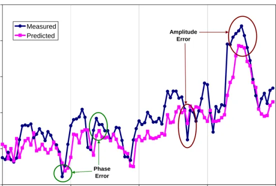
The amplitude and phase errors are illustrated in Figure 3-1 which shows a four-day comparison of the time series of measured and predicted wind speeds at one wind farm. The amplitude error is clearly seen at 17th hour on January 14, 2008. The phase error is more pronounced at 20th hour on January 12, 2008 and 9th hour on January 13, 2008.
Figure 3-1: Comparison of the time series of measured and predicted wind speeds at first forecast horizon (T=1hr) by an anonymous forecaster at a particular wind farm (name is not disclosed). Note examples are circled.
0 5 10 15 20 25 1/12/2008 1/13/2008 1/14/2008 1/15/2008 1/16/2008 Date Winds peed (m/s ) Measured Predicted Phase Error Amplitude Error
Figure 3-2 and Figure 3-3 show the annual MAE and RMSE respectively by region and by forecast horizon for each forecaster. For completeness, the quarterly MAE and RMSE are presented in Appendix D.
Figure 3-2: Annual Mean Absolute Error (MAE) of wind speed (WS) predictions (Pred) in South West (SW), South Central (SC), South East (SE), Central (CE), Existing Facilities (EF), Future Facilities (FF) and All Facilities (AF) by three forecasters A, B and C as a function of forecast horizons.
2 4 6 12 17 24 36 48 1 2 3 4 5 Forecast Horizon (hr) M A E of W S P red . ( m /s ) F o reca st er A W IN D : M A E SW SC SE CE EF FF AF 2 4 6 12 17 24 36 48 1 2 3 4 5 Forecast Horizon (hr) MAE of W S Pr ed . ( m /s ) F o recast er B W IN D : M A E SW SC SE CE EF FF AF 2 4 6 12 17 24 36 48 1 2 3 4 5 Forecast Horizon (hr) M A E of W S P red . ( m /s ) Fo re ca st e r C W IN D : M A E SW SC SE CE EF FF AF
Figure 3-3: Annual Root Mean Square Error (RMSE) of wind speed (WS) predictions (Pred.) in South West (SW), South Central (SC), South East (SE), Central (CE), Existing Facilities (EF), Future Facilities (FF) and All facilities (AF) by three forecasters A, B and C as a function of forecast horizons.
2 4 6 12 17 24 36 48 1 2 3 4 5 Forecast Horizon (hr) R M S E o f W S P re d . (m /s ) F o recas te r A M E T : R M S E SW SC SE CE EF FF AF 2 4 6 12 17 24 36 48 1 2 3 4 5 Forecast Horizon (hr) R M S E o f W S P re d . (m /s ) F o recas te r B M E T : R M S E SW SC SE CE EF FF AF 2 4 6 12 17 24 36 48 1 2 3 4 5 Forecast Horizon (hr) R M S E o f W S P re d . (m /s ) F o recas te r C M E T : R M S E SW SC SE CE EF FF AF
Referring to Figures 3-2 and 3-3, the annual MAE and RMSE, the range of values over the three forecasters for MAE are; from 1.4 to 3.5 m/s and for RMSE from 1.9 to 4.6 m/s. It should be noted that Forecaster A and C show a rapid increase in MAE and RMSE from time horizon T=1 to time horizon T=6 before flattening out while Forecaster B remains relatively flat over all horizons. This difference between Forecasters A and C and Forecaster B is probably due to the forecast methodologies used.
For all forecasters the ordering of the regions for both MAE and RMSE are the same, i.e. the largest MAE and RMSE values are in the SW region and the lowest values are in the Central (CE) region with the other regions falling in between. There are possibly three reasons why the SW region has the largest values and the CE region has the smallest values. As shown on the map of Alberta in Appendix A, the SW region’s topography is more complex than for the CE region, which would indicate that it is more difficult to forecast in the SW region. Secondly, the SW region in relative size to the CE region is much smaller and thus the individual sites are closer together than in the CE region and again may have an effect on forecasting based on topography and spatial smoothing. Finally the winds on average are lighter in the CE regions than in the SW region which can influence the statistic.
3.1.1.1Decomposition of RMSE
Figure 3-4 shows the decomposition of RMSE for the three forecasters. For all forecasters the dispersion (disp) component dominates the RMSE in all regions over all forecast horizons. The disp accounts for the contribution of phase errors to the RMSE. Thus, the largest error in the forecasts is due to phase errors. It should be noted that different regions show a consistent behaviour for disp suggesting a similar property affects all regions in a similar manner. After time horizon T=6 there appears to be a linear increase of dispersion with prediction horizon indicating a systematic growth in the average phase errors between prediction and measurement with increasing lead time.
The second contributor of RMSE seems to be sdbias, the absolute value of which increases steeply for Forecasters A and C until forecast horizon T=6 and remains asymptotic with increasing lead time. Another common feature is the negative sdbias which indicates the variability of the predicted wind speed is smaller than the measured wind speed variability. Model fidelity, as would be expected, limits the forecaster’s ability to predict the finer detail of wind speed.
The bias is the smallest contributor to the RMSE although it seems significant in the Central region for Forecaster A, all regions for Forecaster B and in the South West, South East and Central regions for Forecaster C.
The bias varies in the range of -1.4 to 1.5 m/s. An attempt was made to correlate the bias with the terrain feature, but no commonality was found among the three forecasters. This might indicate the difference in the forecast methodologies employed.
Figure 3-4 Annual errors of wind speed predictions in South West (SW), South Central (SC), South East (SE), Central (CE), Existing Facilities (EF), Future Facilities (FF) and All Facilities (AF) by Forecasters A, B, and C as a function of forecast horizon. Note that RMSE and its components: dispersion (disp), bias (bias) and standard deviation of bias (sdbias) are shown with different symbols and colors.
-2 -1 0 1 2 3 4 SW Errors of P red. W S (m /s ) SC SE 246 12 17 24 36 48 CE Forecast Horizon (hr) 246 12 17 24 36 48 -2 -1 0 1 2 3 4 EF Forecast Horizon (hr) Errors o f P red. W S (m /s ) F o recast er A : W IN D 246 12 17 24 36 48 FF Forecast Horizon (hr) 246 12 17 24 36 48 AF Forecast Horizon (hr)
RMSE DISP BIAS SDBIAS
-2 -1 0 1 2 3 4 SW Errors of P red. W S (m /s) SC SE 246 12 17 24 36 48 CE Forecast Horizon (hr) 246 12 17 24 36 48 -2 -1 0 1 2 3 4 EF Forecast Horizon (hr) Errors o f P red. W S (m /s) F o recast er B : W IN D 246 12 17 24 36 48 FF Forecast Horizon (hr) 246 12 17 24 36 48 AF Forecast Horizon (hr)
RMSE DISP BIAS SDBIAS
-2 -1 0 1 2 3 4 SW E rro rs o f Pre d . W S (m /s ) SC SE 246 12 17 24 36 48 CE Forecast Horizon (hr) 246 12 17 24 36 48 -2 -1 0 1 2 3 4 EF Forecast Horizon (hr) E rro rs of Pre d . W S (m /s ) F o recaster C : W IN D 246 12 17 24 36 48 FF Forecast Horizon (hr) 246 12 17 24 36 48 AF Forecast Horizon (hr)
3.1.2 RMSE and MAE Power
The accuracy of wind power prediction is dictated by different factors including: • The accuracy of wind speed prediction;
• The amplification and dampening of the wind speed prediction error through the nonlinear power curve; and
• Wind farm efficiency including the turbine availability and performance. The overall accuracy of wind speed prediction has been assessed in the previous section. The general accuracy of power prediction is described in this part of the report. Due to the differences in the wind farm efficiency between the Existing Facilities and Future Facilities, the assessment of wind power prediction accuracy is focused on the wind power regions consisting of the existing wind farms, i.e., South West region and South Central region, and Existing Facilities. As noted in the data section (section 2) only 11 months of data were used for the Existing Facilities power analysis since for power prediction the forecasters only had the months of June 2007 to April 2008 period fully populated.
All the error measures described in this section are normalized by the rated wind power capacity.
3.1.2.1Normalized RMSE
Analogous to the wind speed error measures, Figure 3-5 shows the annual normalized RMSE at different forecast horizons in different regions for the three forecasters.
Figure 3-5: Annual Normalized Root Mean Square Error (RMSE %) of Power predictions in South West (SW), South Central (SC), and existing facilities (EF) by three forecasters A, B and C as a function of forecast horizons. Note that the actual errors are normalized by the rated capacity (RC) of the region of power aggregation.
2 4 6 12 17 24 36 48 0 10 20 30 40 Forecast Horizon (hr) No rm . RM SE o f P o we r Pr e d .( % ) F o re cast er A P W R : R M S E SW SC EF 2 4 6 12 17 24 36 48 0 10 20 30 40 Forecast Horizon (hr) No rm . RMS E o f P o we r Pr e d .( %) F o reca st er B P W R : R M SE SW SC EF 2 4 6 12 17 24 36 48 0 10 20 30 40 Forecast Horizon (hr) Nor m . RM SE o f Po wer Pr ed .( % ) F o re cast er C P W R : R M S E SW SC EF
From Figure 3-5, the normalized annual RMSE of the power prediction exhibits a general increase with the increase of forecast horizons, particularly for the first 6 forecast horizons. The normalized RMSE is in the range of 6% to 20% for the first six forecast horizons and 20% to 30% between the 7th and 48th forecast horizon.
The South West (SW) and South Central (SC) regions, which include the Existing Facilities, and have the smallest spatial dimensions as shown in Appendix A, have the highest normalized RMSE. The normalized RMSE is in general lower for regions involving future facilities (not shown here) or with larger spatial dimensions. For the Future Facilities, the measured power was calculated by using power curves and wind speed distributions with a generic wind farm performance, which probably reduces the prediction errors.
As discussed in section 3.1.1, the RMSE can be decomposed into meaningful parts to shed some insight on the different error sources, such as bias as an amplitude indicator, difference between the standard deviations of predicted and measured indicating errors due to wrongly predicted variability, and dispersion indicating the contribution of phase errors to the RMSE. Figure 3-6 shows the decomposition of the RMSE for power. The decomposition of the RMSE for power shows similar traits as for wind.
3.1.2.2Normalized MAE
Figure 3-7 presents the normalized annual MAE. For completeness, the quarterly normalized MAE is presented in Appendix E. The normalized annual MAE shows a general increase with the forecast horizons, particularly for the first 6 forecast horizons, similar to the pattern of the normalized RMSE.
Figure 3-6: Annual Errors of power predictions in South West (SW), South Central (SC), Existing Facilities (EF), by Forecasters A, B, and C as a function of forecast horizon. Note that RMSE and its components: dispersion (disp), bias (bias) and standard deviation of bias (sdbias) are shown with different symbols and colors.
-15 0 15 30 45 SW N o rm . E rro rs (% ) 2 4 6 12 17 24 36 48 SC Forecast Horizon (hr) 2 4 6 12 17 24 36 48 -15 0 15 30 45 EF Forecast Horizon (hr) N o rm . E rro rs (% ) F o recast er A : P O W E R
RMSE DISP BIAS SDBIAS
-15 0 15 30 45 SW N o rm . E rro rs (% ) 2 4 6 12 17 24 36 48 SC Forecast Horizon (hr) 2 4 6 12 17 24 36 48 -15 0 15 30 45 EF Forecast Horizon (hr) N o rm . E rro rs (% ) F o recast er B : P O W E R
RMSE DISP BIAS SDBIAS
-15 0 15 30 45 SW No rm . Er ro rs (% ) 2 4 6 12 17 24 36 48 SC Forecast Horizon (hr) 2 4 6 12 17 24 36 48 -15 0 15 30 45 EF Forecast Horizon (hr) Norm . Errors (% ) F o re c a s te r C : PO W E R
Figure 3-7: Annual Normalized Mean Absolute Error (MAE %) of power predictions in South West (SW), South Central (SC), and existing facilities (EF) by three forecasters A, B and C as a function of forecast horizons. Note that the MAE is normalized by the rated capacity of the region of aggregation.
2 4 6 12 17 24 36 48 0 10 20 30 Forecast Horizon (hr) N o rm . M A E o f P o w e r P re d .(% ) F o rec as te r A P W R : M A E SW SC EF 2 4 6 12 17 24 36 48 0 10 20 30 Forecast Horizon (hr) Nor m . M AE o f Po w e r Pr ed. (% ) Fo reca st e r B P W R : M A E SW SC EF 2 4 6 12 17 24 36 48 0 10 20 30 Forecast Horizon (hr) Nor m . M AE o f Po w e r Pr ed. (% ) Fo reca st e r C P W R : M A E SW SC EF
3.2 What is the accuracy of the Forecasts at the different forecast horizons studied (T=1 hour to T=48 hours)?
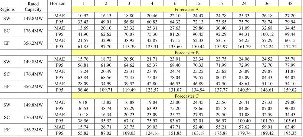
Table 3.1 provides an indication of the accuracy for power at the different forecast horizons, suggested by the working group, for each forecaster. The table presents the Mean Absolute Error and the P95 both in units of power (MW) which is the confidence level at which the Absolute Error does not exceed that value 95% of the time. The rated capacity for each region is also presented. In general the accuracy decreases as the forecast horizon increases. There is a variation between forecasters in accuracy at each forecast horizon. However the trend of decreasing accuracy as the forecast horizon increases is preserved by each forecaster.
Table 3-1: General Accuracy for Power Forecasts for Each Forecaster on an Annual-Base Horizon 1 2 3 4 6 12 17 24 36 48 Regions Rated Capacity Forecaster A MAE 10.92 16.13 18.80 20.46 22.10 24.47 24.78 25.33 26.18 27.20 SW 149.8MW P95 33.43 49.01 56.58 60.83 64.32 72.13 73.55 75.79 78.74 79.94 MAE 13.69 20.10 23.32 25.31 27.63 29.86 30.40 31.09 32.68 34.45 SC 176.4MW P95 41.90 62.62 70.07 75.30 81.26 90.45 92.29 94.31 100.12 99.44 MAE 21.57 32.90 38.95 42.87 47.15 52.33 53.16 54.25 57.29 60.15 EF 356.2MW P95 61.85 97.70 113.39 123.31 133.60 150.44 155.97 161.79 174.24 172.72 Forecaster B MAE 15.76 18.72 20.50 21.71 23.01 23.34 23.75 24.06 24.52 25.78 SW 149.8MW P95 56.81 61.90 64.62 65.37 68.40 70.33 71.99 72.99 72.70 77.99 MAE 17.24 20.49 22.31 23.49 24.74 25.22 25.62 26.89 29.07 31.87 SC 176.4MW P95 63.84 68.56 72.45 75.05 78.04 79.57 80.32 85.09 84.43 94.02 MAE 28.09 34.99 39.52 42.80 46.53 46.89 47.50 48.61 51.10 54.10 EF 356.2MW P95 96.46 109.71 119.49 123.57 131.07 134.94 137.77 140.59 146.61 159.02 Forecaster C MAE 9.18 13.82 16.88 19.04 23.00 24.45 25.56 26.41 27.33 29.00 SW 149.8MW P95 36.53 48.74 57.29 63.93 75.20 78.66 82.18 84.06 87.02 90.82 MAE 10.18 16.34 20.23 23.09 25.72 27.97 29.50 31.08 32.59 34.43 SC 176.4MW P95 38.56 55.52 67.10 75.97 83.67 92.01 96.97 100.40 101.20 105.61 MAE 15.74 26.71 33.75 39.03 47.71 52.40 55.21 57.62 59.91 63.49 EF 356.2MW P95 55.82 87.02 109.03 124.16 151.85 163.18 175.88 179.74 189.42 195.35
3.3 What is the accuracy of the Forecasts at different hours of the day and seasons of the year?
3.3.1 Hours of the Day
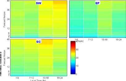
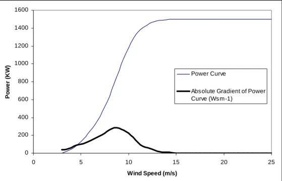
Figure 3-8 presents the annual accuracy of the power forecast for different 6 hour time periods (1-6 hours, 7-12 hours, 13-18 hours and 19-24 hours) of the day for the SW, SC, and EF for the specified forecast horizons for each forecaster. For completeness, the quarterly accuracy of the power forecasts for different 6 hour time periods of the day are provided in Appendix E. While the values for each time of day may vary from forecaster to forecaster it is apparent that the forecasts are the least accurate during the afternoon periods between hours 13 and 18 after forecast horizon T=6. The reason for the less accuracy in the afternoon periods can be accounted for by higher wind speeds and their variability which convert to higher power generation producing larger errors which can be explained by the power conversion curve (see section 3.5, 3.7).
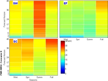
3.3.2 Seasons of the Year
Figure 3-9 shows the accuracy of the power forecasts over the four seasons of the year as indicated by the working group specifically;
• Winter ...November, December, January, February
• Spring...March, April, May
• Summer ...June, July, August
• Fall ...September, October
From Figure 3-9 the lowest accuracy occurs during the winter season for all forecasters while the greatest accuracy is during the summer season. It should be noted that for forecaster B the summer forecasts in the SW region are less accurate than forecasters A and C. When the hourly values (measured vs. forecast) for June through August were examined for Forecaster B in the SW Region there was a much larger deviation from the measured values for July and August than for Forecasters A and C.
The reduced accuracy in the winter season could be due to higher wind speeds and an increased number of weather systems covering the total area during that time of year.
Appendix E contains the accuracy of the power forecasts by month that make up the four seasons of the year.
Figure 3-8: Annual Accuracy of the Power Forecast for Specific 6 Hour Time Periods for Each Forecaster Using RMSE (% Rated Capacity) for the South West (SW), South Central (SC), and Existing Facilities (EF).
Figure 3-9: Seasonal Accuracy of the Power Forecast for Each Forecaster Using RMSE (% Rated Capacity) for the South West (SW), South Central (SC), and Existing Facilities (EF).
3.4 What is the accuracy of the Forecasted Meteorological Data before running through the Power Conversion models?
This question has been addressed in sections 3.1-3.2 by examining the accuracy of the wind speed forecasts.
3.5 What is the accuracy of the Power Conversion?
The error in the power has three components, an error due to an error in the wind speed measurement, a systematic error due to the shape of the power curve and an error due to a lack of an indication of wind farm performance.
The prediction errors in wind speed may be amplified or damped when predicted wind speeds are converted into the wind power prediction. The amplification magnitude depends on the power curve, particularly on the derivative of the power curve at different wind speeds. If the wind farm performance is known, the power conversion errors can be modeled. However, the wind farm performance data was not known to either ORTECH, or to the forecasters at the time when the wind power prediction is issued. Therefore, ORTECH attempted to lump the power conversion error and the effect of the wind farm performance on the prediction errors together by comparing the same error measures, i.e., RMSE and MAE for both the wind speed and power prediction.
In order to facilitate the comparison, both the RMSE and MAE should be normalized at a common scale. The common scale for normalizing the wind speed is the average measured wind speed. For normalizing the power, the common scale is the mean of the measured power because it inherently considers both the turbine type and typical wind speed (reference 3 in the bibliography). The mean values and standard deviations of measured wind speed and power annually are shown in Table 3-2. The relative standard deviation of measured wind, i.e., the ratio of the standard deviation to the average wind speed is in a narrow range between 0.53 and 0.60 in different regions with an exception of 0.47 in the Central (CE) region which has the lowest average measured wind speed. The relative standard deviation of measured power, i.e., the ratio of the standard deviation to the average measured power is in a range between 0.72 and 0.94 in the different regions. The relative standard deviation of measured power is larger than the relative standard deviation of measured wind speed by a factor of 1.23 to 2.02. This factor is due to the power curve and wind farm performance, and could be regarded as a reference value for gauging the power conversion errors. According to reference 3 in the bibliography, if the power was proportional to wind speed cube and the variations in wind speed were small compared to the mean value, this factor would be around 3 corresponding to the average derivative of the power curve.