Nowcasting

Working PaPer SerieS

no 1275 / DeCeMBer 2010

noWCaSting

by Marta Bańbura,

Domenico Giannone

and Lucrezia Reichlin

W O R K I N G PA P E R S E R I E S

N O 1275 / D E C E M B E R 2 010

In 2010 all ECB publications feature a motif taken from the €500 banknote.

NOWCASTING

by Marta Bańbura

1

_{, Domenico Giannone}

2

and Lucrezia Reichlin

3

_,

This paper can be downloaded without charge from http://www.ecb.europa.eu or from the Social Science Research Network electronic library at http://ssrn.com/abstract_id=1717887.

NOTE: This Working Paper should not be reported as representing

the views of the European Central Bank (ECB).

The views expressed are those of the authors

and do not necessarily reflect those of the ECB.

© European Central Bank, 2010 Address

Kaiserstrasse 29

60311 Frankfurt am Main, Germany Postal address

Postfach 16 03 19

60066 Frankfurt am Main, Germany Telephone +49 69 1344 0 Internet http://www.ecb.europa.eu Fax +49 69 1344 6000 All rights reserved.

Any reproduction, publication and reprint in the form of a different publication, whether printed or produced electronically, in whole or in part, is permitted only with the explicit written authorisation of the ECB or the authors. Information on all of the papers published in the ECB Working Paper Series can be found on the ECB’s website, http://www. ecb.europa.eu/pub/scientific/wps/date/ html/index.en.html

Abstract 4

Non-technical summary 5

1 Introduction 7

2 The problem 9

3 The econometric framework 12

3.1 Monthly factor model 13

3.2 Modelling quarterly variables 14

3.3 Estimation and forecasting 15

4 Related literature 16

5 Empirical results 18

5.1 Data set 19

5.2 Forecast updates and news 21

5.3 Forecast uncertainty 22

6 New developments and open problems 26

7 Conclusions 28

References 29

Appendices 33

Abstract

We define nowcasting as the prediction of the present, the very near future and the very recent past. Crucial in this process is to use timely monthly information in order to nowcast key economic variables, such as e.g. GDP, that are typically collected at low frequency and published with long delays. Until recently, nowcasting had received very little attention by the academic literature, although it was routinely conducted in policy institutions either through a judgemental process or on the basis of simple models. We argue that the nowcasting process goes beyond the simple production of an early estimate as it essentially requires the assessment of the impact of new data on the subsequent forecast revisions for the target variable. We design a statistical model which produces a sequence of nowcasts in relation to the real time releases of various economic data. The methodology allows to process a large amount of information, as it is traditionally done by practitioners using judgement, but it does it in a fully automatic way. In particular, it provides an explicit link between the news in consecutive data releases and the resulting forecast revisions. To illustrate our ideas, we study the nowcast of euro area GDP in the fourth quarter of 2008.

Keywords: Nowcasting, News, Factor Model, Forecasting.

Non-technical summary

the very recent past.

Nowcasting is particularly relevant for those key macro economic variables which are col-lected at low frequency, typically on a quarterly basis, and released with a substantial lag. To obtain “early estimates” of such key economic indicators, nowcasters use the information from data which are related to the target variable but collected at higher frequency and released in a more timely manner. For example, euro area GDP, which is the key statistic describing the state of the economy, is only available at quarterly frequency and is released six weeks after the close of the quarter. However, there are several variables related to GDP, such e.g. indus-trial production or various surveys, available at monthly frequency and published with shorter delay. These can be used to construct early estimates of GDP. Key in this process is to use the most up-to-date high frequency information in an environment in which data are released in a non-synchronous manner and with varying publication lags (hence the information sets are characterised by the so called “jagged” or “ragged” edge).

Until recently, nowcasting had received very little attention by the academic literature, although it was routinely conducted in policy institutions either through a judgemental process or on the basis of simple models. Among these simple models are the so called bridge equations, which relate GDP to quarterly aggregates of one or a few monthly series. We argue here that, although the bridge between monthly and quarterly variables is an essential component of nowcasting, the process ideally requires more complex modelling than what is offered by single equation models. This is because it not only requires updating the estimates of the target quarterly variable as new data become available throughout the quarter, but also commenting and interpreting the sequence of revisions of those estimates. Not only do we want to know by how much GDP nowcast has been revised, but also what explains the revision – is it, for example, due to higher than expected readings of industrial production or surveys or both and what weighs the most? In other words, we are interested in relating the part of the monthly release that was previously unexpected, the news, to the revisions of GDP estimates. For this kind of analysis we need to model the joint dynamics of the monthly input data and the quarterly target variable in a unified framework.

In this paper we describe an econometric framework which is designed for this analysis. In this framework all variables are considered within a unified system of equations and hence a meaningful model based news can be extracted and the revisions of the nowcast can be expressed as a function of thesenews. Precisely, we follow the approach proposed by Giannone, Reichlin, and Small (2008) and model the monthly data as a parametric dynamic factor model cast in a state space representation. The problems of jagged edge and mixed frequency are In this paper we definenowcasting as the prediction of the present, the very near future and

translated into a problem of missing data (low frequency variables are considered as high frequency series with periodically missing observations). The Kalman filter techniques are used to perform the projections as they automatically adapt to changing data availability. They are also employed to extract thenews and their contributions to the forecast revisions. Importantly, the factor model representation allows inclusion of many variables, which is a desirable characteristic since many releases might contain relevant information for the target variable. As for estimation, we adopt the approach of Ba´nbura and Modugno (2010) who estimate the model by maximum likelihood. It allows us to deal with several important features of the nowcasting process, such as e.g. presence of a substantial amount of missing observations.

The methodology allows to process a large amount of information and to produce a sequence of nowcasts in relation to the real time releases of various economic data, as it is traditionally done by practitioners using judgement, but it does it in a fully automatic way.

To illustrate our ideas, we provide an application for the nowcast of euro area GDP in the fourth quarter of 2008 and we also present results for annual inflation in 2008.

1

Introduction

Economists have imperfect knowledge of the present state of the economy and even of the recent past. Many key statistics are released with a long delay and they are subsequently revised. As a consequence, unlike weather forecasters, who know what is the weather today and only have to predict the weather tomorrow, economists have to forecast the present and even the recent past. The problem of predicting the present, the very near future and the very recent past is labelled asnowcasting and is the subject of this paper.

Nowcasting is particularly relevant for those key macro economic variables which are col-lected at low frequency, typically on a quarterly basis, and released with a substantial lag. To obtain “early estimates” of such key economic indicators, nowcasters use the information from data which are related to the target variable but collected at higher frequency, typically monthly, and released in a more timely manner. One of the key features of an effective now-casting tool is to incorporate the most up-to-date information in an environment in which data are released in a non-synchronous manner and with varying publication lags.

For example, euro area GDP is only available at quarterly frequency and is released six weeks after the close of the quarter. In March 2010, for instance, we only had information up to the last quarter of 2009 and we needed to wait until mid-May to obtain a first estimate of the first quarter of 2010. However, there are several variables, available at monthly frequency and published with shorter delay, which can be used to construct early estimates of GDP. For example, in mid March comes a release of euro area industrial production for January. These series measure directly certain components of GDP and are considered to contain a strong signal on its short-term developments. Much more timely information, albeit potentially less precise, is provided by various surveys. They measure expectations of economic activity and are typically available shortly before the end of the month to which they refer. Beyond industrial production and surveys, many other data releases are likely to be informative on the state of the economy as it is revealed by the fact that many are closely watched by financial markets which react whenever there are surprises about the value of the new data (for evidence on this point, see Cutler, Poterba, and Summers, 1989).

While in this paper we concentrate the discussion around GDP, the ideas developed here could be applied to nowcasting any low frequency variable released with a substantial delay, for which we can exploit more timely, higher frequency information. The emphasis on GDP is justified by the fact that this is the key statistic describing the state of the economy. In policy institutions, and in particular in central banks, its nowcast is closely monitored and frequently updated to incorporate the information from latest data releases (see e.g. ECB, 2008; Bundesbank, 2009). Further, the nowcast is often used as an input for the more general forecasting process which is concerned with longer horizon and often conducted on the basis

of large structural models.

Until recently, nowcasting had received very little attention by the academic literature, although it was routinely conducted in policy institutions either through a judgemental process or on the basis of simple models. Among these simple models are the so called bridge equations, which relate GDP to quarterly aggregates of one or a few monthly series.

Although the bridge between monthly and quarterly variables is an essential component of nowcasting, as monthly data are more timely than quarterly and they are released more often, nowcasting ideally requires more complex modelling than what is offered by bridge equations. This is because it not only requires updating the estimates of the target quarterly variable as new data become available throughout the quarter, but also commenting and interpreting the sequence of revisions of those estimates. Not only do we want to know by how much GDP nowcast has been revised, but also what explains the revision – is it, for example, due to higher than expected readings of industrial production or surveys or both and what weighs the most? In other words, we are interested in relating the part of the monthly release that For this kind of analysis we need to model the joint dynamics of the monthly input data and the quarterly target variable in a unified framework.

Two seminal papers (Evans, 2005; Giannone, Reichlin, and Small, 2008) have formalized this process in statistical models. Both approaches model, within the same statistical frame-and propose solutions for estimation when data have missing observations at the end of the sample due to non synchro-nized publication lags (the so called jagged/ragged edge problem).1

The model used in this paper is based on Giannone, Reichlin, and Small (2008), but we also rely on several extensions due to Ba´nbura and Modugno (2010). The general framework is a factor modela laForni, Hallin, Lippi, and Reichlin (2000) and Stock and Watson (2002a), but the estimation method is quasi maximum likelihood as in Doz, Giannone, and Reichlin (2006a).

The methodology of Giannone, Reichlin, and Small (2008) has a number of desirable fea-tures and, in particular, it offers a parsimonious solution for the inclusion of a rich information set. Data which are typically watched and commented on throughout a quarter are at least a dozen, but this number can be higher. The model was first implemented at the Board of Gover-nors of the Federal Reserve in a project which started in 2003 and then at the European Central Bank (ECB, 2008). The methodology has also been implemented for other economies, includ-ing various euro area countries (R¨unstler, Barhoumi, Cristadoro, Reijer, Jakaitiene, Jelonek, 1_{The terminologyjagged edgewas first introduced in Giannone, Reichlin, and Small (2008). The more recent} nowcasting literature also uses the termragged edge.

to the revisions of GDP estimates. was previously unexpected, the news,

Rua, Ruth, Benk, and Nieuwenhuyze, 2008; D’Agostino, McQuinn, and O’Brien, 2008), New Zealand (Matheson, 2010) and Norway (Aastveit and Trovik, 2008).

Two results that have emerged from the empirical literature suggest that nowcasting has an important place in the broader forecasting literature. First, Giannone, Reichlin, and Small (2008) show that gains of institutional and statistical forecasts of GDP relative to the na¨ıve constant growth model are substantial only at very short horizons and in particular for the current quarter. This implies that our ability to forecast GDP growth mostly concerns the current (and previous) quarter. Second, Giannone, Reichlin, and Sala (2004) show that the automatic statistical procedure in Giannone, Reichlin, and Small (2008) performs as well as the nowcast published in the Greenbooks, which is the result of a complex process involving models and judgement. For the euro area, similar results are obtained in Angelini, Camba-M´endez, Giannone, R¨unstler, and Reichlin (2008).

Another robust empirical result coming from this work is that the timeliness of data mat-ters, that is the exploitation of early releases leads to improvement in the nowcast accuracy. In particular, the literature shows that surveys, which provide the most timely information, contribute to an improvement of the estimate early in the quarter but by the time hard informa-tion, such as industrial producinforma-tion, becomes available later in the quarter, their contribution vanishes (Angelini, Camba-M´endez, Giannone, R¨unstler, and Reichlin, 2008; Ba´nbura and R¨unstler, 2010; Giannone, Reichlin, and Small, 2008; Matheson, 2010).

We should stress that, related to nowcasting, is a literature on coincident indicators of economic activity where, rather than focusing on an early estimate of GDP, an unobserved state of the economy is estimated from a multivariate model. Although some of the problems in this literature are related to those described above for nowcasting, in this chapter we do not review this literature in much detail and limit the discussion to pure nowcasting defined as timely estimation and its analysis of a particular target variable such as GDP.

The chapter is organized as follows. The second section defines the problem of nowcasting in general and relates it to the concept ofnewsin macroeconomic data releases briefly described above. In the third section, we explain the details of our approach. In section four we discuss related literature while, in section five, we illustrate the characteristics of the model via an application to the nowcast of GDP and inflation in the euro area. Section six discusses issues for further research and the last section concludes.

2

The problem

Before referring to a particular model, let us define formally the general problem of producing a nowcast and its updates, which arise as a result of an inflow of new information.

in the introduction, GDP is released only six weeks after the close of the reference quarter. In the meantime it can be estimated using higher-frequency, namely monthly, variables that are published in a more timely manner.

To describe the problem more formally, let us denote by Ω_v a vintage of data available at time _v, where_v refers to the date of a particular data release. Further let us denote GDP growth at time_tas_ytQ. We define the problem of nowcasting of_yQ_t as the orthogonal projection of_yQ_t on the available information set Ω_v:

PyQ_t|Ω_v =E yQ_t |Ω_v , (1) whereE ·|Ω_v

refers to the conditional expectation. One of the elements that distinguish nowcasting from other forecast applications is the structure of the information set Ω_v. One particular feature is typically referred to as its “ragged” or “jagged edge”. It means that, since data are released in a non-synchronous manner and with different degrees of delay, the time of the last available observation differs from series to series. Another feature is that it contains mixed frequency series, in our case monthly and quarterly. Hence we will have Ω_v = {_{xi,ti, ti} = 1_,2_{, ..., Ti,v, i}= 1_{, ..., n} ;_yQ_3k,3_k = 3_,6_{, ..., TQ,v}} where _Ti,v corresponds to the last period for which in vintage _v the series_i has been observed.2 _{Because of the}

non-synchronicity of data releases,_Ti,v is not the same across variables and therefore the data set exhibits the above mentioned jagged edge.

Hence the problem of nowcasting needs to be analyzed in a framework which imposes a plausible probability structure on Ω_v and which can efficiently exploit all the relevant infor-mation from such an inforinfor-mation set, where, in particular, the number of potential monthly predictors,_xi,t, could be large.

jection for a quarter of interest but rather a sequence of nowcasts, which are updated as new data arrive. The first nowcasts are usually made with very little or no information on the reference quarter. With subsequent data releases they are revised, leading to more precise projections as the information on the period of interest accrues. In other words we will, in general, perform a sequence of projections: E

yQt|Ωv , E ytQ|Ωv+1 , ..., where _v, _v+ 1, ..., refer to dates of consecutive data releases. Typically the intervals between two consecutive data releases are short (possible couple of days or less) and change over time. Consequently, vhas high frequency and is irregularly spaced.

We now explain why and how the nowcast is updated and introduce the concept of news

which is central to understanding the nowcast revisions.

2_{Given our definition of nowcast as prediction of the present, the very near future and the very recent past,} and maxiTi,v is usually small and can be negative. Ω_v could possibly include more quarterly variables, we limit this set to GDP for the sake of simplicity.

pro

the difference between the forecast reference period _t

Let us first analyse the difference between the two information sets Ω_v and Ω_v+1. At time v+ 1 we have a release of certain group of variables, {_{xj,Tj,v+1, j} ∈ J_v+1} and consequently the information set expands.3 _{The new information set differs from the preceding one for}

two reasons. First, it contains new, more recent figures. Second, old data might get revised. In what follows we will abstract from the problem of data revisions. Therefore, we have Ω_v ⊆Ω_v+1and Ω_v+1\Ω_v ={_{xj,Tj,v+1, j}∈J_v+1}.

Given the “expanding” character of the information and the properties of orthogonal pro-jections we can decompose the new forecast as:

EyQ_t|Ω_v+1 new forecast =E y_tQ|Ω_v old forecast +E yQ_t|Iv+1 revision , (2)

where_Iv+1 is the subset of the information set Ω_v+1 whose elements are orthogonal to all the elements of Ω_v. Given the difference between Ω_v and Ω_v+1 specified above, we have that

Iv+1,j =xj,Tj,v+1−E

xj,Tj,v+1|Ωv

and_Iv+1= (_{Iv+1,1. . . Iv+1,Jv+1}), where_Jv+1denotes the number of elements inJ_v+1. Hence, the only element that leads to a change in the nowcast is the “unexpected” (with respect to the model) part of the data release,_Iv+1, which we label as thenews. The concept of news

is useful because what matters in understanding the updating process of the nowcast is not the release itself but the difference between that release and what had been forecast before it. In particular, in an unlikely case that the released numbers are exactly as predicted by the model, the nowcast will not be revised. On the other hand, we would intuitively expect that e.g. a negative news in industrial production should revise the GDP forecasts downwards. Below we show how this can be quantified.

It is worth noting that the news is not a standard Wold forecast error. First of all, the pattern of data availability changes with time. Second, the news depends on the order in which new data are released.

From the properties of the conditional expectation, we can further develop (2) as:

EyQt |Iv+1 =E ytQIv+1 EIv+1Iv+1 −1 Iv+1. (3)

In order to expand (3) further and to extract a meaningful model-basednews component, one needs to have a model which can reliably account for the joint dynamic relationships among the data. Given such model and assuming that the data are Gaussian, it turns out that we can find coefficients_bj,t,v+1 such that:

EyQt|Ωv+1 new forecast =E ytQ|Ωv old forecast + j∈Jv+1 bj,t,v+1 xj,Tj,v+1−E xj,Tj,v+1|Ωv news .

3_{Typically one “additional” observation is released and we haveT}

j,v+1=Tj,v+ 1 for allj∈Jv+1. GDP could be also included in a release, we abstract from this case in order not to complicate the notation.

In other words we can express the forecast revision as a weighted sum of news from the released variables: EyQ_t|Ω_v+1 −EyQ_t|Ω_v forecast revision = j∈Jv+1 bj,t,v+1 xj,Tj,v+1−E xj,Tj,v+1|Ωv news . (4)

Hence, consistent with the intuition, the magnitude of the forecast revision depends, on one hand, on the size of thenews and, on the other hand, on its relevance for the target variable as quantified by the associated weight _bj,t,v+1.

Decomposition (4) enables us to trace the sources of forecast revisions back to individual predictors. In the case of a simultaneous release of several (groups of) variables it is possible to decompose the resulting forecast revision into contributions from the news in individual (groups of) series therefore allowing commenting the revision of the target in relation to unexpected developments of the inputs. This decomposition is also useful when the forecast is updated less frequently than at each new release (we provide an illustration in the empirical section).

3

The econometric framework

To compute nowcasts, news and their contributions to nowcast revisions all we need is, in principle, to perform linear projections. In practice, we have to deal with several problems including mixed frequency, jagged edge and possibly other cases of missing data and the curse of dimensionality due to the richness of the available information which, if included, can lead to imprecise and volatile estimates.

In this paper we follow the approach proposed by Giannone, Reichlin, and Small (2008) who offer a solution to these problems by modelling the monthly data as a parametric dynamic factor model cast in a state space representation. Once we obtain the state space representa-tion, the Kalman filter techniques can be used to perform the projections as they automatically adapt to changing data availability. Importantly, the factor model representation allows inclu-sion of many variables, which is a desirable characteristic since many releases

As for estimation, we adopt the approach of Ba´nbura and Modugno (2010) who estimate the model by maximum likelihood. Doz, Giannone, and Reichlin (2006a) have shown that the maximum likelihood approach is feasible and robust in the context of large scale factor models. It also allows us to take into account several important features of the nowcasting process as it is illustrated in the next section.

The next subsections describe the model and the estimation in detail.

might contain relevant information for the target variable.

3.1

Monthly factor model

We start by specifying the dynamics for the monthly data. How to include quarterly variables within this framework is discussed in the next subsection.

Let_xt= (_{x1,t, x2,t, . . . , xn,t}) denote the monthly series, which have been transformed to satisfy the assumption of stationarity. More precisely, _xt are month-on-month growth rates (or differences) of the original variables, see the Appendix for details on the transformations applied. We assume that_xtobey the following factor model representation:

xt = _μ+ Λ_ft+_εt, (5)

where _ft is a_r×1 vector of (unobserved) common factors and_εt is a vector of idiosyncratic components. Λ denotes the factor loadings for the monthly variables. The common factors and the idiosyncratic components are assumed to have mean zero and hence the constants μ= (_{μ1, μ2, . . . , μn}) are the unconditional means. Further, the factors are modelled as a VAR process of order _p:

ft = _A1ft−1+· · ·+_Apft−p+_{ut, ut}∼_{i.i.d. N}(0_{, Q})_, (6) where _{A1, . . . , Ap} are_r×_rmatrices of autoregressive coefficients.

Finally, we assume that the idiosyncratic component of the monthly variables follows an AR(1) process:

εi,t = _αiεi,t−1+_{ei,t, ei,t}∼_{i.i.d. N}(0_{, σ}2_i)_, (7)

withE[_ei,tej,s] = 0 for_i=_j.

Taking explicitly into account the dynamics of the factors is particularly important in nowcasting applications. The reason is that, due to publication delays, the information on the most recent periods can be scarce and exploiting the dynamics, in addition to contemporaneous relationships, can increase the precision of the factor estimates.

In contrast to models typically used in the context of nowcasting, we further restrict Λ,_A1, ...,_Apand_Q. Specifically, we partition_ftinto mutually independent global, real and nominal factors. We assume that the global factor is loaded by all the variables while real and nominal factors are specific to real and nominal variables, respectively. Precisely, assuming (without loss of generality) that all the nominal variables are ordered before the real, we have:

Λ = Λ_N,G Λ_N,N 0 Λ_R,G 0 Λ_R,R , ft= ⎛ ⎝ f G t ftN ftR ⎞ ⎠_{, Ai}= ⎛ ⎝ Ai,G0 _Ai,N0 00 0 0 _Ai,R ⎞ ⎠_{, Q}= ⎛ ⎝ QG0 _QN0 00 0 0 _QR ⎞ ⎠_,

where labels _G, _N and_R correspond to the global, nominal and real factors, respectively. This framework is used to account for the local cross-sectional correlation within the real and nominal blocks, which is helpful for a more efficient extraction of the global factor. This type of restriction is easily accommodated within maximum likelihood approach to estimation as discussed below. Of course, this approach also allows implementation of other structures, e.g. more local factors for a finer grouping of the variables.

Doz, Giannone, and Reichlin (2006a) have shown that, for large cross-sections, the model given by (5) can be estimated by maximum likelihood under the assumption of lack of serial and cross-sectional correlation in the idiosyncratic component even if this condition is not satisfied by the data. However, this mis-specification can cause problems in small samples and consequently in nowcasting because of the incomplete cross-sections at the end of the sample. Explicit modelling of serial correlation of the idiosyncratic component and including local factors aims at mitigating this problem.4

3.2

Modelling quarterly variables

We follow Mariano and Murasawa (2003) and incorporate quarterly variables into the frame-work by constructing for each of them a partially observed monthly counterpart.

Lets us explain it on the example of GDP. In what follows we adopt the convention in which the value of the quarterly variable is “assigned” to the third month of the respective quarter. Accordingly, quarterly level of GDP, which we denote by_GDPtQ_{, t}= 3_,6_,9_{, ...}, can be expressed as the sum of its unobserved monthly contributions, _GDPtM:

GDPtQ=GDPtM +GDPtM−1+GDPtM−2, t= 3,6,9, ...

Let us define _YtQ = 100×log(_GDPtQ) and _YtM = 100×log(_GDPtM). We assume that the unobserved monthly growth rate of GDP, _yt = Δ_YtM, admits the same factor model representation as the monthly real variables:

yt = _μQ+ Λ_Qft+_εQ_{t ,} (8)

εQ_t = _αQεQ_t−1+_eQ_{t , e}Q_t ∼_{i.i.d. N}(0_{, σ}2_Q)_, (9) with Λ_Q= (Λ_Q,G 0 Λ_Q,R).

To link_ytwith the observed GDP data we construct a partially observed monthly series:

yQt =

YtQ−YtQ−3, t= 3,6,9, ...

unobserved_, otherwise

and use the approximation of Mariano and Murasawa (2003):

y_tQ = _YtQ−_YtQ₋₃≈(_YtM +_YtM₋₁+_YtM₋₂)−(_YtM₋₃+_YtM₋₄+_YtM₋₅)

= _yt+ 2_yt−1+ 3_yt−2+ 2_yt−3+_{yt−4, t}= 3_,6_,9_{, ...} (10) 4_{Explicit modelling of the dynamics of idiosyncratic component can be also useful to forecast variables with} strong non-common dynamics.

3.3

Estimation and forecasting

Let us define ¯_xt = (_{xt, y}Q_t) and ¯_μ = (_{μ, μQ}). The joint model specified by the equations (5)-(10) can be cast in a state space representation:

¯

xt= ¯_μ+_Z(_θ)_αt,

αt=_T(_θ)_αt−1+_{ηt, ηt}∼ _{i.i.d. N}(0_,Σ_η(_θ))_, (11) where the vector of states includes the common factors and the idiosyncratic components. In the case_p≤5, we have

αt= (_{ft, ft−1, ft−2, ft−3, ft−4, ε1,t, . . . , εn,t, ε}Q_{t, ε}Q_{t−1, ε}Q_{t−2, ε}Q_{t−3, ε}Q_t−4)_.

Q 1 1 n Q, σ1, . . . , σn,σQ,

are collected in_θ. The details of the state space representation, and in particular the structure of the matrices,_Z(_θ),_T(_θ) and Σ_η(_θ), are provided in the Appendix.5

In this paper, we estimate _θ by maximum likelihood implemented by the Expectation Maximisation (EM) algorithm. This approach has been proposed for large data sets by Doz, Giannone, and Reichlin (2006a) and extended by Ba´nbura and Modugno (2010) to deal with missing observations and idiosyncratic dynamics. Giannone, Reichlin, and Small (2008) used a different procedure involving two steps: first the parameters of the model are estimated using principal components as factor estimates; second, factors are re-estimated using the Kalman filter (see Doz, Giannone, and Reichlin, 2006b). Roughly speaking, the maximum likelihood estimation using the EM algorithm consists in iterating the two-step approach: estimating the parameters conditional on the factor estimates from previous iteration and vice versa.

Maximum likelihood allows us to easily deal with such features of the model as substantial fraction of missing data, restrictions on the parameters or serial correlation of the idiosyn-cratic component. In addition, as we also study models of moderate sizes (less than 30 vari-ables), maximum likelihood approach should be more efficient. Finally, in this framework, it is straightforward to introduce factors that are specific to a subgroup of variables, see above. The details of the EM iterations, following Ba´nbura and Modugno (2010), are given in the Appendix.

Given an estimate of_θ, the nowcasts as well as the estimates of the factors or of any missing observations in ¯_xt, can be obtained from the Kalman filter or smoother. Precisely, under the assumption that the data generating process is given by (11) with_θequal to its QML estimate,

projection (1) for any pattern of data availability in Ω_v.6 _{One way to understand how the}

5_{For the sake of simplicity in the presentation we assume that there is only 1 quarterly variable, GDP. However,} it is straightforward to incorporate more quarterly variables, see the Appendix.

6_LetT

v= maxi{Ti s.t.x¯i,Ti ∈Ωv}. The Kalman filter will be used in case the target periodtin (11) is equal

or larger thanT_v. The Kalman smoother will be used otherwise.

, _Q, _{α , . . . , α} , _α All the parameters of the model, _μ¯, Λ, Λ ,_A

the Kalman filter and smoother can be used to obtain, in an efficient and automatic manner, , . . . , Ap

Kalman filter and smoother deal with missing data is to imagine that they simply discard the rows in ¯_xtand_Z(_θ) that correspond to the missing observations in the former vector, see e.g. Durbin and Koopman (2001).

In addition, thenews _Iv+1 and the expectations needed to compute_bj,t,v+1 in (4) can be also easily retrieved from the Kalman smoother output, see Ba´nbura and Modugno (2010) for details. It is worth noting that for_tlarge enough so that the Kalman filter has approached its steady state, the weights _bj,t,v+1 will not depend on a particular realisation of{_xj,T¯ _{j,v+1, j}∈

Jv+1} but only onθand on the shape of the jagged edge in Ωv and Ωv+1.

4

Related Literature

Our approach, as described in the previous section, relies on the assumption that the data are driven by few unobservable factors. Recent applications of the factor model approach are Angelini, Camba-M´endez, Giannone, R¨unstler, and Reichlin (2008), R¨unstler, Barhoumi, Cristadoro, Reijer, Jakaitiene, Jelonek, Rua, Ruth, Benk, and Nieuwenhuyze (2008), Ba´nbura and R¨unstler (2010), Camacho and Perez-Quiros (2010), Marcellino and Schumacher (2008) amongst others. The model by Evans (2005) is similar in spirit and is based on the assumption that GDP is the only unobservable factor.

A key feature our modelling strategy is that it relies on a unified system of equations that summarises the joint dynamics of the target variable and the predictors. The problems of jagged edge and mixed frequency are translated into a problem of missing data. The latter can be dealt with efficiently through the application of the Kalman filter as the system has a state space representation. These features enable us to obtain, for any pattern of data availability, forecasts of all the variables, allowing for a model based interpretation of the nowcast updates in terms of news.

In this section we briefly review alternative modelling strategies that have been proposed for nowcasting or related problems.

The traditional approach to nowcasting, which has been implemented at various central banks, is the bridge equation solution. It is a single equation framework in which the nowcast is obtained from a regression of the quarterly target variable on its lags and on some monthly predictors. In order to retain parsimony in lag specification for the monthly variables, they are converted to the frequency of the target variable, typically using equal weights. In case there is only partial monthly information on a given quarter, auxiliary models – for each of the monthly predictors or for their subgroups – are used to infill the “missing” months. Early applications of bridge equations are Trehan (1989) or Parigi and Schlitzer (1995) and examples of more recent applications are Parigi and Golinelli (2007), R¨unstler and S´edillot (2003), Kitchen and Monaco (2003) and Diron (2008), amongst others.

More recently, in a literature which does not focus on nowcasting, Ghysels, Santa-Clara, and Valkanov (2004) have proposed another solution to forecasting low frequency variable with high frequency predictors - so called MIDAS (Mixed Data Sampling) regressions. It is also a single equation approach, however it does not require the frequency conversion as it involves a parsimoniously parameterized distributed lag polynomial for the high frequency regressors. As a consequence, more distant lags can be included and no auxiliary forecasting equations are necessary. On the other hand, model parameters depend on forecast horizon and on the pattern of data availability. In the context of nowcasting MIDAS has been applied by e.g. Clements and Galv˜ao (2008) and Marcellino and Schumacher (2008) who also evaluate it against alternative approaches.

Single equation approaches described above are simple and can be quite effective. In case of parameters instability they can be also more robust compared to a system solution. However, from the perspective of nowcast interpretation they have an important drawback, namely they do not produce a system based forecast for all the variables. This hinders a rigorous understanding of nowcast revisions in terms of news embedded in consecutive data releases. One way to get around this problem is proposed by Ghysels and Wright (2009) who assess the effect of news on the updates of the nowcasts and forecasts by considering expectations from survey data and using auxiliary regressions to link the survey based news with the revisions of the model forecast.

Let us turn to the problem of estimation. The approach followed in this paper is based on the EM algorithm for a dynamic factor model that can deal with a general pattern of missing data. Stock and Watson (2002b) developed an algorithm based on the principle of the EM for the extraction of principal components from panels with missing data and mixed frequency. Their approach, however, is not well suited for news extraction and revision inter-pretation since, when forecasting the missing observations, one only considers cross-sectional dependence, while the time dependence is ignored. Schumacher and Breitung (2008) apply the approach of Stock and Watson (2002b) to nowcast German GDP from monthly data and forecast the periods for which no (or no sufficient) data is available via an auxiliary forecasting model (VAR) for the factors.

As regards including data sampled at mixed frequencies into a state space representation the approximation for the growth rates of Mariano and Murasawa (2003)7_{results in a linear model}

but implies that the monthly interpolations of the levels are inconsistent with the quarterly totals. In the context of nowcasting, this approach has been used by Angelini, Camba-M´endez, Giannone, R¨unstler, and Reichlin (2008) and Ba´nbura and Modugno (2010) amongst others. 7_{Mariano and Murasawa (2003) in a context of a model aimed at constructing a coincident index of aggregate} economic activity rather than at nowcasting.

Mitchell, Smith, Weale, Wright, and Salazar (2005) and Proietti (2008) propose alternative approaches which do not use approximation (10) and ensure that the sum of estimates of the monthly levels of GDP is consistent with the observed quarterly figure.

Regarding the literature on coincident indicators of economic activity, a classic paper in this field is Stock and Watson (1989). More recently, new ideas on how to construct these indicators have led to the Eurocoin index for the euro area (Altissimo, Bassanetti, Cristadoro, Forni, Hallin, Lippi, and Reichlin, 2001; Altissimo, Cristadoro, Forni, Lippi, and Veronese, 2006) and the Chicago Fed index for the US (ChicagoFED, 2001). Aruoba, Diebold, and Scotti (2009) are posting a similar index,

data, in the Philadelphia Fed website. It is worth noting that the former two papers adopt a different solution to the jagged edge problem than applied in this paper. ChicagoFED (2001) uses auxiliary models to forecast missing observations. The strategy in Altissimo, Bassanetti, Cristadoro, Forni, Hallin, Lippi, and Reichlin (2001) and Altissimo, Cristadoro, Forni, Lippi, and Veronese (2006) is to shift particular variables in order to obtain a data set that is complete at the end of the sample. For example, if there is one more month available for surveys than for industrial production, we can realign the two series by dating industrial production referring to month _t−1 as a time _t observation.8 _{In this case, the model used for the projection is}

not time invariant since it changes with the pattern of data availability. For this reason the

5

Empirical results

In this section we illustrate the ideas developed above by employing the model described in Section 3 to forecasting of quarter-on-quarter GDP growth and of annual inflation. The purpose is to illustrate how the real time data flow shapes the evolution of consecutive forecast updates. More precisely, we examine how releases of different groups of data revise the forecast and affect the associated forecast uncertainty.

For each target variable and each reference period we consider a sequence of forecast updates. These are produced twice a month at dates which correspond, approximately, to the releases of major groups of hard and soft data (in the middle and at the end of each month, respectively).

We are also interested in the role of more disaggregated sectoral data. To this end we compare the performance of a benchmark model that contains mainly aggregated data with the results from a richer data set including sectoral information. Such disaggregated data are routinely monitored by sectoral experts and can be important not only to eventually improve 8_{These methods have been compared empirically with the Kalman filter solution used in this paper by Marcellino} and Schumacher (2008) and R¨unstler, Barhoumi, Cristadoro, Reijer, Jakaitiene, Jelonek, Rua, Ruth, Benk, and Nieuwenhuyze (2008).

which is based also on higher frequency (weekly)

forecast accuracy but also for understanding and interpreting the forecasts. Most of the factor models used in central banks for nowcasting are based on large disaggregated data sets. However, sectoral information can lead to model mis-specification in small samples since it introduces idiosyncratic cross-correlation. Hence, the comparison is interesting to understand the robustness of the model with respect to the inclusion of many variables.

In all the exercises we assume 1 global, 1 real and 1 nominal factor (hence the total number of factors is_r= 3) and one lag in the factor VAR (_p= 1).

5.1

Data set

Let us first comment on the data set for our benchmark model. It contains twenty-six major indicators on the euro area economy. The series are presented in Table 1. As mentioned above, most of the series relate to the total economy. The only exception are surveys which are disaggregated into major sectors. This can be important as surveys are the only monthly source of information on services.

The data set contains mainly monthly series and such is the frequency of our model. Data with the native frequency higher than monthly are aggregated as monthly averages. The exception are commodity prices, which enter as averages over the first 15 days of a month and hence, for a given month, are available already in its middle.9

In the table we also report respective publication delays (in days). There are substantial differences between the series in terms of their timeliness. For example survey and financial series, which are sometimes labelled as soft data, are already available at the end of the respective reference period (or even couple of days before). In contrast, hard data on real activity are released with 2-3 months delay. However, they typically carry a more precise signal for GDP developments. Since there is likely to be a tradeoff between timeliness and precision, the data set is constructed to contain both “timely” soft data and “precise” hard data. The last two columns of Table 1 report the (stylised) data availability patterns, or the “shape” of the jagged edge, that we apply for the bi-monthly forecast updates.

The disaggregated data set contains a sectoral split for industrial production, more detailed labor market information as well as few more quarterly series. A detailed list is provided in the Appendix.

9_{Monthly averages would have been smoother but also less timely. Empirical results indicate that considering} more timely information on commodity prices is more optimal for inflation. More systematic analysis on inclusion of higher frequency is left for future research.

T

able

1:

Data

set

No Group Series F requency Publication dela y No of missing observ ations (in da ys after reference p erio d) mid mon th end mon th 1 Real, Hard data IP , total industry Mon thly 37-40 22 2 Real, Hard data IP , man ufacturing Mon thly 32-35 22 3 Real, Hard data Retail trade, except for motor v ehicles and motorcycels Mon thly 33-39 22 4 Real, Hard data New passenger car registrations Mon thly 15-17 11 5 Real, Hard data New orders, man ufacturing w orking on orders Mon thly 42-45 32 6 Real, Hard data Extra euro area trade, exp ort, v alue Mon thly 44-48 32 7 Real, Hard data Unemplo ymen t rate, total Mon thly 29-32 22 8 Real, Hard data Index of emplo ymen t, total industry Mon thly 80-140 4,5,3 4,3,3 9 Real, Surv eys Purc hasing manager index, man ufacturing Mon thly -10 10 Real, Surv eys Purc hasing managers surv ey , services, business activit y Mon thly -10 11 Real, Surv eys Consumer surv ey , consumer confidence indicator Mon thly -10 12 Real, Surv eys Industry surv ey , industrial confidence indicator Mon thly -10 13 Real, Surv eys Retail trade surv ey , retail confidence indicator Mon thly -10 14 Real, Surv eys Services surv ey , services confidence indicator Mon thly -10 15 Nominal, HICP HICP , o v erall index Mon thly 15-18 11 16 Nominal, PPI PPI, total industry excluding construction Mon thly 32-35 22 17 Nominal, Surv eys Consumer surv ey , price trends o v er next 12 mon ths Mon thly -10 18 Nominal, Surv eys Industry surv ey , selling price exp ectations for the mon ths ahead Mon thly -10 19 Nominal, Money M3, index of notional sto c ks Mon thly 25-29 21 20 Nominal, Money Index of loans Mon thly 25-29 21 21 Real, Financial Do w Jones Euro Sto xx, broad sto c k exc hange index Daily -10 22 Nominal, Financial Eurib or 3 mon ths Daily -10 23 Nominal, Financial Nominal effectiv e exc h. rate, core group of currencies against euro Daily -10 24 Nominal, Comm prices Ra w materials excl. energy , mark et prices Daily -10 25 Nominal, Comm prices Ra w materials, crude oil, mark et prices Daily -10 26 Real, GDP Gross domestic pro duct, c hain link ed Quarterly 42-44 4,2,3 4,2,3 Notes: Fifth column of the table indicates typical publication dela y (in da ys) for eac h series. on config uration of business da ys. “-” means “no publication dela y”, suc h series are a v ailable directly at the end of the reference p erio d (or couple of da ys b efore). Base d on a typical publication dela y , w e rep ort in sixth and sev en th column a (st ylised) n um b er of missing observ ations at the end of the sample in the middle and at the end of a mon th. F or emplo ymen t index and GDP w e rep ort 3 n um b ers (corresp onding to first, second and third mon th of eac h quarter) as these series are not released eac h mo n th. W e use these data a v ailabilit y patterns in the forecast ev aluation exercises. It ma y v ary from mon th to mon th, dep ending e.g.

5.2

Forecast updates and news

As an illustration, we first produce a sequence of forecast updates for GDP growth rate in Since inflation is available at monthly frequency and with short publication lags, it is not our focus. However, having a model that can consider jointly prices and quantities is potentially useful for interpreting results.

For the GDP we consider bi-monthly updates of next, current and previous quarter fore-casts. Specifically, we produce a first forecast with data available in mid July 2008 and we subsequently update it at two-week intervals, each time incorporating new data releases.10

The resulting six updates performed from July till September target the next-quarter GDP growth. With the update from mid-October till end-December we effectively project current quarter GDP growth. The last two updates are performed in January 2009 and they refer to the previous quarter (the flash estimate for 2008 Q4 GDP was released in mid February). In some applications next, current and previous quarter forecasts are labelled as “forecasts”, “nowcasts” and “backcasts”, respectively.

Concerning HICP, we proceed in a similar manner. We produce the first forecast in mid-July and we update it twice a month up to end of December 2008 (HICP is typically released around two weeks after the end of the reference period).11

The evolution of the forecast for both variables as produced by our model is depicted in Figure 1. In the same chart, we report the contribution of thenewscomponent of the various data groups to the forecast revision.12 _{As explained in Section 2, the difference between two}

consecutive forecasts, i.e. the forecast revision, is the sum over all the released variables of the product of thenewsrelated to a particular variable and the associated weight in the GDP estimate (see equation (4)). The contribution of thenewsfrom a block of variables is the sum of contributions of the series belonging to this block. The composition of different blocks is indicated in the second column of Table 1. To make the graphs easier to read, certain groups have been merged. In the case of GDP forecast, e.g. all nominal variables constitute a single group.

Let us comment on the evolution of the GDP forecast. At the beginning of the forecasting period the forecast remains rather flat, corroborating the above mentioned difficulties in fore-10_{The exercises in this and in the next section are pseudo real time, that is, we follow a stylised publication} calendar and we do not account for data revisions.

11

on-month growth rates of prices. Since prices enter the data set as month-on-month growth rates, the forecast for For example in mid-July we already observe the monthly growth rates for the first half of the year and need to forecast only the remaining 6 months.

12

2008. the fourth quarter of 2008 and for the annual inflation in December

Using the logarithmic approximation of a growth rate, annual inflation can be expressed as a sum of 12 month-annual inflation is obtained as sum of partially observed and partially forecast month-on-month growth rates.

For each forecast sequence the parameters are estimated only once, before the first forecast in the sequence is made, and kept constant for all the subsequent forecast updates.

casting beyond the current quarter. The first substantial downward revision (pointing to a negative GDP growth) comes with the release of surveys for October, which is the first block of real data referring to the current quarter. This negative news in October is confirmed by subsequent data, both surveys and hard data. In fact, with all subsequent releases the forecasts are revised downwards. In addition, later in the reference quarter, the news from the hard data block become more sizeable. This is in line with the results of Giannone, Reichlin, and Small (2008) and Ba´nbura and R¨unstler (2010) who show that less timely hard data become important only later in the forecast sequence. The contribution of the nominal block is rather limited throughout the whole forecast cycle.

Concerning HICP inflation, the largest revisions are caused by the releases of HICP itself and of commodity prices. These seem to be the most informative data sources on the short-term developments in inflation. In contrast, the contribution of thenewsfrom the surveys on prices and from the real block is relatively small. The same is true fornews on other nominal variables such as money, exchange rate or interest rates.

Some caution should be taken when reading the results since our model assumes constant parameters. The downturn has been rather deep relative to what was experienced during the sample and hence parameter instability and stochastic volatility might have played an important role (for a recent study see Mitchell, 2009). Our model assumes that the parameters are stable, this is an important limitation although there are some results concerning the robustness of factor models to parameters instability, see e.g. Stock and Watson (2008).

5.3

Forecast uncertainty

Uncertainty around the nowcast related to signal extraction at any point in time can be easily evaluated using the Kalman filtering techniques (see Giannone, Reichlin, and Small, 2008). However, these estimates only hold under the the assumption that errors are Gaussian and that the model is well specified. To overcome these limitations we will assess forecast uncertainty by evaluating the average historical performances of the model.

To this end, we perform a simulated pseudo real time forecasting exercise. This means that at each point in time we estimate the parameters of the model and produce forecasts using the data that replicates the pattern of data availability at the time. Estimating the model recursively takes into account estimation uncertainty.

We are, in particular, interested in how uncertainty evolves as the information related to the target period accrues. Since the bi-monthly updates described in the previous section differ in terms of available information, we examine the average accuracy for each of them separately. As the measure of uncertainty we choose the Root Mean Squared Forecast Error (RMSFE) and we evaluate it over the period 2000-2007. The resulting uncertainty for our

Figure 1: Contribution of news to forecast revisions

GDP growth QoQ 2008 Q4 -1.25 -1.00 -0.75 -0.50 -0.25 0.00 0.25 0.50 mid Jul 0 8 end Jul 0 8 mid Aug 08 end Aug 08 mid Sep 08 end Sep 08 mid Oct 08 end Oct 08 mid Nov 08 end Nov 08 mid Dec 08 end Dec 08 mid Jan 09 end Jan 09 Real, Hard data Real, Surveys Real, Financial Nominal Fcst

HICP inflation YoY Dec 2008 -0.80 -0.40 0.00 0.40 0.80 1.20 1.60 2.00 mid Jul 0 8 end Jul 0 8 mid Aug 08 end Aug 08 mid Sep 08 end Sep 08 mid Oct 08 end Oct 08 mid Nov 08 end Nov 08 mid Dec 08 end Dec 08 1.20 1.60 2.00 2.40 2.80 3.20 3.60 4.00 Nominal, HICP Nominal, Surveys Nominal, Comm prices Nominal, Other Real Fcst (rhs)

Figure 2: Unconditional uncertainty around the forecast

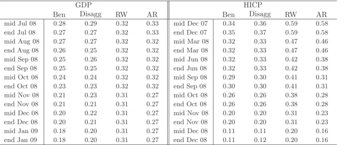
*'3JURZWK4R4 4 PLG -XO HQG-X O PLG $XJ HQG$XJ PLG 6HS HQG6 HS PLG 2FW HQG2 FW PLG 1RY HQG1R Y PLG 'HF HQG'HF PLG -DQ HQG-D Q %HQ 5: +,&3LQIODWLRQ<R< 'HF PLG 'HF HQG'HF PLG 0DU HQG0D U PLG -XQ HQG -XQ PLG 6HS HQG6 HS PLG 2FW HQG2 FW PLG 1RY HQG1R Y PLG 'HF HQG'HF %HQ 5:

Table 2: Forecast uncertainty

GDP HICP

Ben Disagg RW AR Ben Disagg RW AR

mid Jul 08 0.28 0.29 0.32 0.33 mid Dec 07 0.34 0.36 0.59 0.58

end Jul 08 0.27 0.27 0.32 0.33 end Dec 07 0.35 0.37 0.59 0.58

mid Aug 08 0.27 0.27 0.32 0.32 mid Mar 08 0.32 0.33 0.47 0.46

end Aug 08 0.26 0.25 0.32 0.32 end Mar 08 0.32 0.33 0.47 0.46

mid Sep 08 0.25 0.26 0.32 0.32 mid Jun 08 0.32 0.33 0.42 0.38

end Sep 08 0.25 0.25 0.32 0.32 end Jun 08 0.32 0.33 0.42 0.38

mid Oct 08 0.24 0.24 0.32 0.32 mid Sep 08 0.29 0.30 0.41 0.31

end Oct 08 0.23 0.23 0.32 0.32 end Sep 08 0.30 0.30 0.41 0.31

mid Nov 08 0.21 0.23 0.31 0.27 mid Oct 08 0.26 0.26 0.38 0.28

end Nov 08 0.21 0.21 0.31 0.27 end Oct 08 0.26 0.26 0.38 0.28

mid Dec 08 0.20 0.22 0.31 0.27 mid Nov 08 0.20 0.20 0.31 0.23

end Dec 08 0.20 0.21 0.31 0.27 end Nov 08 0.20 0.20 0.31 0.23

mid Jan 09 0.18 0.20 0.31 0.27 mid Dec 08 0.11 0.11 0.20 0.16

end Jan 09 0.18 0.20 0.31 0.27 end Dec 08 0.11 0.12 0.20 0.16

Notes: Table provides forecast uncertainty for quarter-on-quarter GDP and annual HICP for different models. Benrefers to the benchmark model with 26 variables, see Table 1. Disagg refers to the specification with more disaggregated data, see the Appendix. RW denotes random walk with drift model for levels of logged GDP and random walk without drift for annual inflation. ARrefers to an autoregressive model for quarterly growth rates of GDP and monthly growth rates of HICP. Uncertainty is given by the Root Mean Squared Forecast Error evaluated over the period 2000-2007. Dates in the first columns indicate data availability patterns with These availability patterns were applied recursively in the forecast evaluation.

benchmark model is depicted in Figure 2. On the _x-axis we use the same labels as in Figure 1 to indicate that the average uncertainty was computed with the same data availability assumptions, relative to the target period. There is a slight difference in the chart for inflation as for RMSFE we also consider longer forecast horizons.

For comparison we plot the same average uncertainty measure for forecasts produced by univariate na¨ıve models. For GDP it is the random walk with drift for the levels of logged GDP. For HICP it is the driftless random walk for the annual inflation.

We can observe that, as the information accumulates, the gains in forecast accuracy are substantial. For GDP the RMSFE is reduced by 50% as we move from the first to the last forecast in the sequence. For “earlier” forecasts larger gains are obtained when surveys are released (the decreases in RMSFE corresponding to end-month releases are larger). When hard data for the reference quarter become available, surveys lose their importance. This suggests that soft data are relevant due to their timeliness but, conditionally on the availability of hard data for the same reference period, they are uninformative. This confirms the results in Giannone, Reichlin, and Small (2008), Ba´nbura and R¨unstler (2010) and Matheson (2010). We also note that the uncertainty measures associated with next quarter forecasts for the benchmark and na¨ıve model are comparable, confirming earlier results about the difficulties of forecasting beyond the current quarter. This also applies to institutional forecasts (see Giannone, Reichlin, and Small, 2008).

Decreasing uncertainty corresponding to the inclusion of the newly published data as we proceed throughout the quarter is also true for HICP inflation. We gain in forecast accuracy mostly due to mid-month releases, corresponding to the release of the HICP itself and of commodity prices.

Finally let us compare the results with forecast accuracy of the model including more dis-aggregated data. Table 2 reports the corresponding RMSFE based uncertainty. We also recall the results for the benchmark and random walk models and in addition consider autoregressive univariate models.

The exercise based on disaggregated data shows that including more variables does not improve the accuracy of the forecast but does not affect its stability. Since, in e.g. the preparation of policy briefings, it might be necessary to comment on many releases including disaggregated data, this is good news. Our framework is robust to the inclusion of a rich data set.

6

New developments and open problems

Factor models are not the only solution to the problem of nowcasting. In principle, any dynamic model that can handle mixed frequencies and missing observations and that can capture the

joint dynamics of the target and the predictor variables can be used. Different examples in the literature are Evans (2005) or the VAR proposed by Zadrozny (1990) and Giannone, Reichlin, and Simonelli (2009). Frequentist approach to VAR estimation is, however, not suitable when one needs to handle more than a few series. A promising line for future research is to build on ideas in Ba´nbura, Giannone, and Reichlin (2010) to develop nowcasting tools based on VARs where Bayesian shrinkage is used to cope with the curse of dimensionality problem.

Another idea for further research is to link the high frequency nowcasting framework with a quarterly structural model in a model coherent way. Giannone, Monti, and Reichlin (2009) have suggested a solution and other developments are in progress. A byproduct of this analysis is that one can obtain real time estimates of variables that can only be defined theoretically such as the output gap or the natural rate of interest.

Finally, let us mention that the framework presented here has some limitations.

First, the revision process is not taken into account. Although Giannone, Reichlin, and Small (2008) point out that factor models are robust to data revisions if revision errors among different variables are poorly cross-correlated, modelling explicitly the interplay between data revisions and nowcasting is an import line for future research. Evans (2005) is a first step in this direction. His approach is to model the revision process for GDP only imposing the assumption that revisions are noise. The challenge is to parsimoniously model the revision process for all variables allowing for both noise and news.

Second, we do not incorporate data at frequencies higher than monthly. The model we base our discussion on can be updated at any frequency (minute, day, week, ....) as data are released but includes only monthly and quarterly variables. Financial variables, for example, are converted to monthly frequency and treated as being released only when information on the entire month is available. Although the model can be adapted to properly take into account high frequency data, this is still unfinished work. Aruoba, Diebold, and Scotti (2009) is a first attempt to deal with this problem. They use a small factor model and apply it to the construction of a coincident indicator of the state of the economy rather than to the nowcasting problem. Andreou, Ghysels, and Kourtellos (2008) propose an alternative approach based on MIDAS but treat the predictors as predetermined. The challenge is to model higher frequency within a joint model in order to maintain the ability of understanding the nowcast updates in terms of news.

Last but not least, we do not consider parameters instability and stochastic volatility. This is an interesting line for future research on nowcasting. The challenge there consists in allowing for general forms of time variations within a parsimonious set-up.

7

Conclusions

In this paper we definenowcasting as the prediction of the present, the very near future and the very recent past.

Key in this process is to use timely monthly information in order to nowcast low frequency variables that are published with long delays. We have argued that the nowcasting process goes beyond the simple production of an early estimate and it requires the analysis of the link between thenewsin consecutive data releases and the resulting forecast revisions for the target variable. We have described an econometric framework which is designed for this analysis. In this framework all variables are considered within a single system and hence a meaningful model based news can be extracted and the revisions of the nowcast can be expressed as a function of thesenews.

The methodology allows to process a large amount of information and to produce a sequence of nowcasts in relation to the real time releases of various economic data, as it is traditionally done by practitioners using judgement, but it does it in a fully automatic way. It is used to complement economic analysis in many central banks.

To illustrate our ideas, we have provided an application for the nowcast of euro area GDP in the fourth quarter of 2008 and also presented results for annual inflation in 2008.