REPORT OF INVESTIGATION 25 STATE OF ILLINOIS
OTTO KERNER, Governor
DEPARTMENT OF REGISTRATION AND EDUCATION WILLIAM SYLVESTER WHITE, Director
Selected Methods for
Pumping Test Analysis
by JACK BRUIN and H. E. HUDSON JR.
ILLINOIS STATE WATER SURVEY WILLIAM C.ACKERMANN, Chief
URBANA Third Printing, 1961
REPORT OF INVESTIGATION 25
STATE OF ILLINOIS OTTO KERNER, Governor
DEPARTMENT OF REGISTRATION AND EDUCATION WILLIAM SYLVESTER WHITE, Director
SELECTED METHODS FOR
PUMPING TEST ANALYSIS
by JACK BRUIN and H. E. HUDSON, JR.
STATE WATER SURVEY DIVISION WILLIAM C. ACKERMANN, Chief
URBANA First Printing, 1955 Second Printing, 1958
TABLE OF CONTENTS Page SUMMARY 5 INTRODUCTION 6 Scope of Report 6 Acknowledgments 6 GENERAL 6 Historical 6 System of Units 7 NON-EQUILIBRIUM METHOD 8
Analysis of Test Data 8 Type Curve Solution 8 Example of Analysis 11 Estimation of Future Pumping Water Levels 16
MODIFIED NON-EQUILIBRIUM METHOD 17
Analysis of Test Data 17 Drawdown Method 17 Recovery Method 19 Estimation of Future Pumping and Non-Pumping Water Levels 19
Self-caused Drawdown 21
Interference 21 Areal Recession 22 The Future Pumping and Non-Pumping Water Levels 22
AQUIFER OF LIMITED AREAL EXTENT 22
Hydrologic Boundaries 22 Example of Analysis 26 Recharge Boundaries 27 STEP DRAWDOWN TESTS 29
General Discussion 29 Example of Analysis 30 COMPLICATING FACTORS 36 REFERENCES 38 APPENDIX I 39 APPENDIX II 47 Introduction 49 The Pumped Well 49 Pumping Equipment 50 Observation Wells 50 Period Prior to Test 50 Notes Concerning Collection of Data 50
5
SUMMARY The report describes and illustrates four types of
pumping test data analysis which at present are exten sively used in analysis of problems involving Illinois wells. These methods are, the non-equilibrium "type curve" method, the modified non-equilibrium "straight line" method, the step-drawdown analysis developed by Water Survey staff members, and the analysis of an aquifer that has limited areal extent.
The pumping test is one of the most useful tools avail able in the evaluation of groundwater producing forma tions. The material in this report is designed to meet the present needs of engineers who deal with groundwater in Illinois. So far as possible the details of theories involved have been omitted. Substituted for them are general dis cussions of the applicability of the various types of analy sis. Attention is called to the advantages, disadvantages
and possible mis-use of the equations presented. The assumptions upon which the various types of analysis are based are also discussed.
The "type curve" method is of particular value when observation wells are available and the aquifer being tested is of large areal extent and when the pumping test is of too short duration to use the straight-line meth od. The "straight line" method is applicable when ob servation wells are available and when the testing period is sufficiently long to warrant its use. The analysis of an aquifer of limited areal extent is an adaptation of the "straight line" method to meet the conditions when one or more boundaries of the aquifer are in the vicinity of the well being pumped. The step-drawdown analysis yields information primarily concerning the performance of the well itself rather than the aquifer and does not usually require observation wells.
6
SELECTED METHODS
FOR GROUNDWATER RESOURCES EVALUATION By
Jack Bruin, Assistant Engineer and
H. E. Hudson Jr., Head, Engineering Sub-Division Illinois State Water Survey Division, Urbana, Illinois
INTRODUCTION Scope of Report
This report presents elements of established pumping test analysis procedure which are valuable and beneficial to professional and practicing engineers, well contractors and drillers, municipal and industrial operators, and others interested in the future planning and development of groundwater resources. The report includes a limited number of cases for which well-substantiated clear-cut solutions could be worked out. This report contains ref erences to the literature germane to those cases.
The derivations and proofs of equations have been eliminated. The equations are presented in their devel oped form with a discussion of their applicability and shortcomings. An example of each method is presented
by analyzing an actual pumping test that was not com plicated by recharge considerations.
Acknowledgments
The suggestions and constructive criticisms of Mr. H. F. Smith, Engineer, State Water Survey Division, were of great value in the preparation of this report.
The authors are indebted to the engineers of the State Water Survey Division who have collected data from ap proximately 1300 pumping tests during the past 20 years.
The writers are especially indebted to Mr. Francis X. Bushman, formerly Assistant Engineer, State Water Survey Division, for his work in preparing the Historical section.
GENERAL Historical
The analysis of the hydraulics of wells for the evalu ation of groundwater potentialities by pumping tests falls in the category of groundwater hydrology. This field has been rapidly developed since the publication of the well-known law of flow through porous materials by Henri Darcy in 1856. (1)* This law states that the discharge
through porous media is proportional to the product of the hydraulic gradient, the cross-sectional area normal to the flow and the coefficient of permeability of the material.
In 1863, Dupuit(2) applied Darcy's law to well hy
draulics, using an ideal case of a well located at the center of a circular island.
The Dupuit formula was modified by Thiem( 3 ) in 1906
to a form which is applicable to more general problems. Similar formulas were also advanced by Slichter(4),
Turneaure and Russell(5), Israelson(6), Muskat(7), and
Wenzel(8). However, all of these were essentially either
modified or specialized forms of Dupuit's relationship. These methods may all be classed together as the "equi librium method'' which applies only to a steady-state condition in which the rate of flow of water toward the well is equal to the rate of discharge of the pumped well. A remarkable advance in modern well hydraulics was made through the development of the non-equilibrium theory by Theis( 9 ) of the U. S. Geological Survey in
1935. This theory introduced the time factor and the co-*Numbers refer to the list of references on page 34.
efficient of storage; it made possible the computation of future pumping levels when the flow of groundwater due to pumping did not approach an equilibrium condition.
However, the use of the Theis formula in determining the coefficients of transmissibility and storage-the for mation constants of an aquifer- presented much difficulty because of mathematical complexities in applying the formula, which contains an exponential integral. Theis suggested a graphical method to Wenzel(10) and Jacob(11),
respectively, in 1937 and 1938, for a more practical so lution of this problem. The method was described by Jacob in 1940 and by Wenzel in 1942.
In 1944, Wenzel and Greenlee(12) presented a gener
alization of Theis' graphical solution by which the co efficients may be determined from tests of one or more discharging wells operated at varied rates.
Furthermore, Cooper and Jacob(13) have introduced
an approximation into the non-equilibrium method which results in a method which is convenient to use.
Both the equilibrium and the non-equilibrium methods assume that the water-bearing material is homogeneous and isotropic. This assumption is probably never true in a natural aquifer. However, these methods give reliable results in actual cases when there is no hydrologic boun dary existing within the effective area of pumping. Ex tended application of the equilibrium method to the problems involving hydrologic boundaries was made by Muskat(14) in 1937 by the method of images.
In 1941, Theis(15) illustrated the application of his
non-equilibrium formula to a special boundary problem in which the effect of a well on the flow of a nearby
7 stream was considered.
In 1948, Ferris(16) applied the method of images in
the use of the non-equilibrium theory to the general treatment of simple boundary problems.
The Illinois State Water Survey became very active in promoting production tests of wells during the early 1920's. Much of this promotion work was done by per sonal contact with water well contractors, consulting engineers, and municipal officials. As a result numerous measurements of production rates and water levels for individual wells became available. Under the leadership of the late G. C. Habermeyer, Engineer of the Survey, the use of electric droplines for water level measurements became standard practice for Survey engineers prior to 19259.(24)
For the period 1920-30, Water Survey records reveal eight pumping tests conducted by Survey personnel. The total number of pumping tests on record in the Survey files through 1954 is 1,321.
The first test on record in the Survey files by Survey personnel was conducted on a municipal well at Lawr-enceville in 1922.
The Illinois State Water Survey has used the method of images, based on Ferris' procedure, in a number of cases where the data indicated the existence of boundary conditions, either impermeable or recharge, and in a few cases where both effects were observed.
The Survey has used the non-equilibrium method and most of its modifications in approximately half of the pumping tests conducted since 1946, all of which involved the estimation of future conditions. While making these analyses the characteristics of individual wells have also been studied.
Survey engineers have made a thorough review of the literature on the subject. Much of it pertains to cases for which good examples have not been encountered in Illinois.
The importance and need of this phase of science becomes apparent when one notes the great number of water uses. No living thing exists without water. Noting the progress of groundwater hydrology in the past 20 years or so one may hold forth great hope for future develop ments and expansions of existing facilities.
System of Units
The system of units used in this report is consistent throughout except for the units of time which may be in seconds, minutes, or days as specified. In addition, the units of volume may be specified in either gallons or cubic feet. The units most commonly used in water well pumping test analysis in the State of Illinois are as follows:
Q = Pumping rate in gallons per minute (gpm). t = Elapsed time in minutes or days measured from
the time pumping began or ended.
r = Distance -in feet measured from some reference point, (usually measured from the axis of the dis charging well to another well or location involved in analysis of a particular groundwater problem). s = Drawdown in feet at the well or at any distance
from the well (measured from the non-pumping level).
h= Water level in feet measured from reference ele vation, (usually measured from center line of pump discharge, top of well casing, or ground surface elevation).
m = Thickness of aquifer in feet.
P = Coefficient of permeability of the aquifer. De fined as the rate of flow of water in gallons per day which will move through one square foot of a given aquifer with a unit hydraulic gradient under prevailing conditions.
This is numerically equal to the "field coefficient of permeability (Pf)" which Meinzer defined as ". . . the rate of flow of water, in gallons a day, under prevailing con ditions, through each foot of thickness of a given aquifer in a width of 1 mile, for each foot per mile of hydraulic gradient."(17)
T = Coefficient of transmissibility of the aquifer. De fined as the rate of flow of water in gallons per day which will flow through one foot width of a given aquifer with a unit hydraulic gradient un der prevailing conditions. Transmissibility is the product of aquifer thickness and aquifer perme ability.
y = Specified Yield. Defined as the net quantity of water, in cubic feet, released from storage from a vertical column of aquifer, one-foot square and the height of the saturated portion of the aquifer when one-foot depth of the aquifer is dewatered under prevailing conditions.
8
S = Coefficient of storage. Defined as the net quan tity of water in cubic feet released from storage from a vertical column of aquifer, one-foot
square and the height of the saturated portion of the aquifer, when the hydraulic pressure on the column is reduced one-foot of water under pre vailing conditions.
For water table conditions, S = y.
NON-EQUILIBRIUM METHOD The non-equilibrium method as presented by Theis(9)
in 1935 has been used and studied extensively since its development. It has been verified and modified by the leading authorities in groundwater hydrology. When the field conditions approximate the assumptions made in the development of the theory, the results are strikingly reliable.
The non-equilibrium method as presented by Theis and later developed further by Wenzel(10) is based on
the following assumptions:
(1) the aquifer is homogeneous and isotropic, (2) the aquifer is of infinite areal extent and con
stant thickness,
(3) the discharge well has an infinitesimal diameter and completely penetrates the thickness of the aquifer,
(4) water taken from storage in the aquifer is dis charged instantaneously with the decline in head. In an idealized aquifer fulfilling the above assump tions, the general equations which define the flow toward a pumped well penetrating the entire thickness of the aquifer are as follows:
where
s = drawdown at any point in the aquifer. Q - discharge of pumped well.
T= coefficient of transmissibility of the aquifer, t = time since pumping started in days,
r = distance from the discharging well. S = coefficient of storage of the aquifer.
The solution of equation (II) is too tedious for frequent use. Wenzel(10) has provided a simplified solution through
a table of values of W(u) for a wide range of values of u. Table I provides the values of W(u) for values of u from 9.9 to 1.0 x 10" . A portion of this table is reproduced in graphic form in Figure 1. The values of u and W(u) can be obtained from this graph with sufficient accuracy for most practical purposes. (For greater accuracy the reader is referred to Table 1.)
Analysis of Test Data
Of the variables in the non-equilibrium equations, s, Q, r, and t may be measured during pumping tests. This leaves four unknowns [T, S, W(u), and u] to be determined from the three equations. If no information is available on the unknowns, an exact analytical solution is impos sible . However, methods have been developed which yield solutions of sufficient accuracy for engineering purposes. Type Curve Solution. A graphical method of super position described by Wenzel(10) yields a relatively sim
ple solution of the non-equilibrium equations.
The first step of the "type curve" analysis is to plot values of s (drawdown in an observation well) versus the product of the square of the distance (r2) from the axis
of the pumped well and the reciprocal of the time (t = time in days since pumping began when s is meas ured). These data should be plotted on logarithmic tracing paper. The curve in Figure 1 should be plotted on a sheet of logarithmic tracing paper to the same scale and will be called the "type curve". In making these graphs, s and W(u) should be on the same axes (usually the ordi nate) of their respective graphs. Consequently and u
9
TABLE 1
VALUES OF W(u) FOR NON-EQUILIBRIUM FORMULA
11 would be on the same axes (usually the abscissa) of their
respective graphs. The "type curve" should consist of a smooth curve while the pumping test data curve (s vs ) should consist of only the plotted individual points.
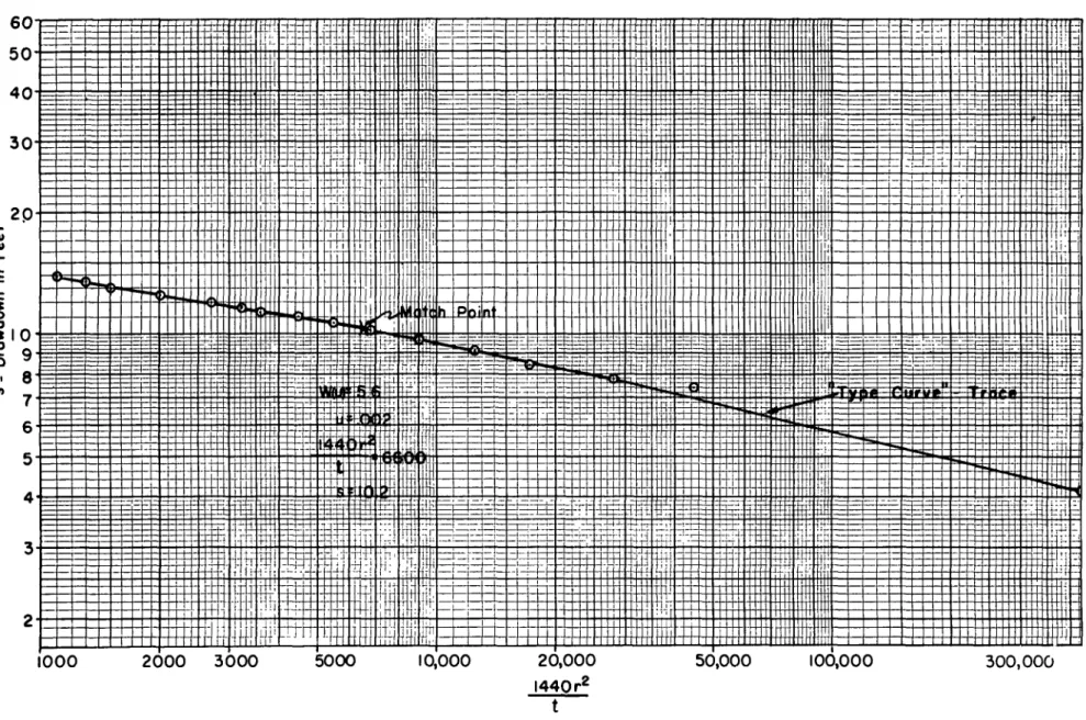
The next step is to place one of the graphs on top of the other and fit the points of the graph to the type curve. This can easily be done with the use of an illumi nated tracing table. If numerous analyses are to be made, it is convenient to have a permanent "typecurve" con structed on transparent material. For accurate work, the minimum size for the permanent type curve should cor respond to 11 × 17 inch 5 × 3 cycle logarithmic graph paper. In fitting the plotted data to the type curve the coordinate axes of the two graphs must be kept parallel. When the "best fit" is obtained by eye, a "match-point" is selected, at any point desired on the fitted curve and marked on both curves. The values of s, W(u), and u to be used in calculating T and S are the values obtained from the "match-point" of the graphs. The values of T and S are computed from equations (I) and (III) in the following forms:
where s, Q, T, t, r, and S are as defined above. The following illustrative analyses will make this procedure clear.
Example of Analysis. The well production test report dated October 9, 1952 for Well No. 1 at the Village of Arrowsmith, Illinois presents the details of the well con struction and the pumping test data (See Appendix II).
It should be noted that it was not possible to measure the water levels in the pumped well but water levels were measured in an observation well 12.5 feet away. The data from the test should make it possible to calcu late the values of the formation constants (T and S) and to estimate the future water level recessions in the vicin ity of the well that would result from pumping the well at various rates. The water level in the well cannot be predicted from these data with precision since the obser vation well data do not reflect the head lost by the water as it enters the well and flows up the well to the pump intake (known as well loss).
The first step in the analysis of the data involves simple calculations. Determine the time in minutes (t) after pumping began at which each water level observa tion was made. Square the distance (r 12.5) from the pumped well and divide it by the time in days at which the water level observations were made. Since there are 1440 minutes in a day this latter calculation becomes , Next, determine the drawdown, which is the
water level in the observation well at the time of each observation minus the level before pumping began, i.e. the amount the water has lowered in the observation well since pumping began. The results of these calculations are shown on the test data sheet of the October 6 test in Appendix II. The next step is to plot the values of versus the drawdown for each value of t on log arithmic graph paper. On another sheet of similarpaper, plot a "type curve" of the values of W(u) and (u) de rived from Table I. Figure 1 is a segment of the "type curve".
Compare the plotted test data with the type curve by a suitable method that permits placing one sheet of pa per on top of the other so that plottings on both sheets may be seen simultaneously. Place the sheet with the plotted test data on top of the "type curve" with the axis parallel to the u-axis and the drawdown s-axis parallel to the W(u)-axis. The top sheet is shifted (always being careful to keep the axes parallel) until the plotted points of the test data are matched up with the "type curve" to make the best possible "eye fit" of the type curve through the plotted points of the test data. It is now usually advisable to trace that portion of the "type curve'' which fits the test data on the data sheet in order to keep a record of the fit obtained. While both sheets are still in this "best fit" position a "match-point" is chosen on the "best fit" portion of the " type curve" and marked. From this match point, record from the test data sheet corresponding values of and drawdown and, from the type curve, corresponding values of W(u) and u. The results of this procedure are illustrated in Figure 2.
Knowing the constant pumping rate of the test to be 250 gallons per minute, everything needed to solve for T and S by means of equations (I a) and (III a) is now available.
Knowing T and S it is now possible to use equations (I) and (III) to estimate the future water levels at any distance (r) from the pumped well and at any time (t) after pumping starts.
For example, assume the anticipated pumping sched-ule will require an average pumpage of 200 gpm for the first year at which time the rate would be increased to 300 gpm until the fifth year when a maximum antici-pated pumpage of 350 gpm would be reached. It is de-sired to know what the pumping level will be at the end of ten years.
The problem is approached in the following manner. Calculate the theoretical water levels at various distances from the well at various times and rates. In this case the calculations were made for the following convenient conditions, using the original pumpage and the incre-mental increases in pumping rates.
times - 1 day, 365 days, 1825 days, 3650 days pumping rates - 50 gpm, 100 gpm, 200 gpm distances - 1 ft, 10 ft, 100 ft, 1000 ft time = 1 day
Q = 50 gpm from equation (III),
u-In equation (I b) S50 is the drawdown for a pumping rate of 50 gallons per minute. In equation (I b) the value of W(u) is dependent on the value of (u) which in turn depends on the values of (r) and (t). The constant 2.74 is dependent on the pumping rate. Therefore, in order to obtain the drawdown at other pumping rates equation (I b) need only be multiplied by the ratio of the desired pumping rate to 50 gpm. Thus for a pumping rate of 100 gpm:
13 The water levels may conveniently be calculated in the following tabular form:
r 1 u 0.303 × 10⁻⁶ W(u) 14.42 5.26 10.52 21.06 10 0.303 × 10⁻⁴ 9.83 3.59 7.18 -14.46 100 0.303 × 1 0- 2 5.23 1.91 3.86 7.69 1000 0.303 0.90 0.33 0.66 1.32 r u W(u) S50 S100 S200 1 8.3 × 10⁻¹⁰ 20.33 7.42 14.84 29.90 10 8.3 × 10⁻⁸ 15.73 5.74 11.48 23.13 100 8.3 × 10- 6 11.12 4.06 8.12 16.35 1000 8.3 × 10⁻⁴ 6.52 2.38 4.76 9.59 r u W(u) S50 S100 S200 1 1.66 × 1 0- 1 0 21.94 8.00 16.00 32.25 10 1.66 × 1 0- 8 17.34 6.32 12.65 25.48 100 1.66 × 10⁻⁶ 12.73 4.65 9.30 18.73 1000 1.66× 10⁻⁴ 8.13 2.97 5.94 11.97 r u W(u) S50 S100 S200 1 8.3 × 10⁻¹¹ 22.64 8.26 16.53 33.29 10 8.3 × 1 0- 9 18.03 6.58 13.16 26.47 100 8.3 × 1 0- 7 13.42 4.90 9.80 19.74 1000 8.3 × 10- 5 8.82 3.22 6.44 12.97
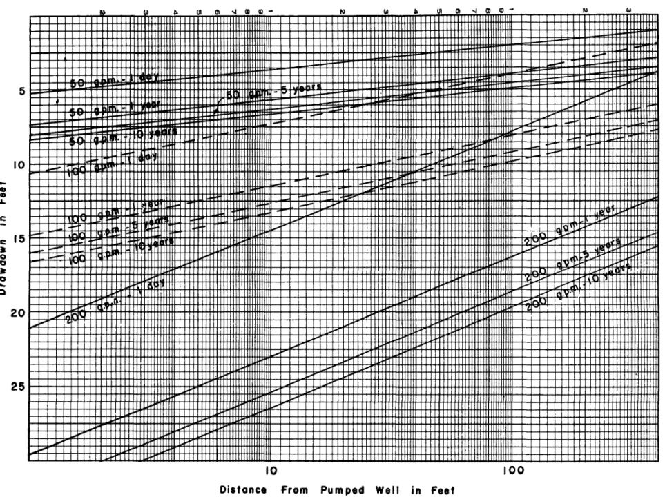
From these calculations three families of curves were plotted on semi-logarithmic graph paper which show the drawdown in the formation at any distance from 1 to 1000 feet from the well while pumping at 50, 100, or 200 gpm for 1 day, 1 year, 5 years, and 10 years (see
16
Fig. 3). From this graph it is possible to combine esti-mates of future water levels that would be found in an observation well located at any distance between 1 and 1000 feet from the pumped well during the next 10 years for the expected schedule of pumping (200 gpm the first year, 300 gpm for the next four years, and 350 gpm for the next five years).
Estimation of Future Pumping Water Levels
The measured non-pumping water level prior to the pumping test was 99.45 feet, but for convenience, it was assumed that at the start of the 10-year schedule the non-pumping level was 100 feet. The non-pumping water levels will be estimated for a point in the aquifer 1 foot from the center of the pumping well.
From Figure 3 it is found that while pumping at 200 gpm, the drawdown one foot from the well is about 21 feet after pumping 1 day, 29.6 feet after 1 year, 32 feet after five years, 33 feet after 10 years (2 latter values extrapolated). By adding the non-pumping level to the drawdown the following data are obtained:
Water Levels While Pumping at 200 GPM Time Since Water Level in Feet Pumping Begun from Ground Surface
1 day 121 365 days (1 year) 129.6
1625 days (5 years) 132 3650 days (10 years) 133 These data were plotted to obtain the 200 gpm curve in Figure 4. This curve gives the estimated levels for the first 365 days and a base curve for obtaining the levels after the pumpage is increased to 300 gpm.
To obtain the water levels after increasing the pump-age to 300 gpm, data from the 100 gpm curve (Fig. 3) are added to those from the 200 gpm curve. It is con-venient to do this in the following tabular form.
Time since pumping began 1 year 2 years 6 years 11 years Time since increase of 100 gpm 1 day 1 year 5 years 10 years Pumping level for 200 gpm 129.6 130.6 132.2 133.2 Drawdown for increase of 100 gpm 10.5 14.8 16.0 16.5 Pumping level for 300 gpm 140.1 145.4 148.2 149.7
The pumping levels for 200 gpm are obtained from Figure 4 and the drawdown for the increase of 100 gpm is obtained from Figure 3 as done previously for the 200 gpm curve. The 300 gpm pumping levels are then plotted on Figure 4.
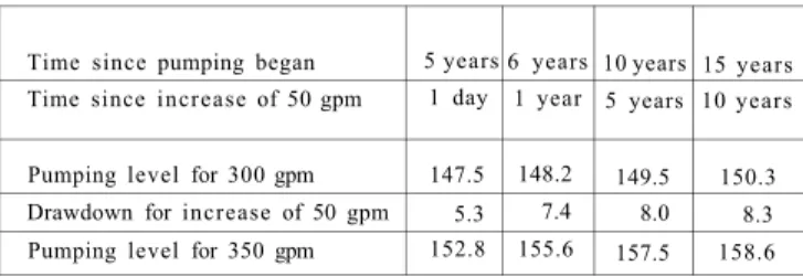
The 350 gpm pumping levels are found similarly:
Time since pumping began 5 years 6 years 10 years 15 years Time since increase of 50 gpm 1 day 1 year 5 years 10 years Pumping level for 300 gpm 147.5 148.2 149.5 150.3 Drawdown for increase of 50 gpm 5.3 7.4 8.0 8.3 Pumping level for 350 gpm 152.8 155.6 157.5 158.6
To aid in drawing the slope of the last limb of the predicted levels, one additional point was calculated for a time of 20,000 days after the increase to 350 gpm. Calculation of drawdown at 1 foot from the pumped well after 20,000 days of pumping at 50 gpm follows:
The solid curve in Figure 4 shows the estimated water levels at a distance of one foot from the pumped well, for the 10-year schedule of pumping.
Figure 4 indicated that the water level one foot from the pumped well would be about 157.5 feet below the top of the casing. Since the depth to the top of the water-producing formation is 223 feet below the top of the casing of the pumped well, the remainder of about 65 feet of head are available to take care of additional losses in and near the well.
The calculations indicate that the formation is ca-pable of yielding the assumed amount of water. These calculations were made under the assumptions listed on page 7 and must be viewed in the light of what the actual conditions may be. During the short (about 4-1/2 hours) pumping test no hydrologic boundaries were noted but this particular formation is known to have bound-aries. These might be located by a study of geologic information available for the area, in which case the pumping levels could be adjusted for these conditions. If the boundaries are sufficiently close, their location could be verified by a longer pumping test using more observation wells. The methods of dealing with various boundary conditions are illustrated in other examples of pumping test analysis. Unless the areal extent of the aquifer has previously been determined to be extremely large by long pumping tests or other means, it would not be conservative to base the design of a water system on so short a test of the source of supply as was used for this illustration.
17 MODIFIED NON-EQUILIBRIUM METHOD
A very simple method for determining the formation coefficients was introduced by Cooper and Jacob( 1 3 ) in 1946. It is a modification of the Thies non-equilibrium method. Cooper and Jacob have shown that when plotted on semi-logarithmic paper, the theoretical drawdown curve approaches a straight line when sufficient time has elapsed after pumping started.
In many instances plotting of the data while the test is in progress reveals whether the straight-line regime is being attained. However, the gentle transition into the straight line is sometimes hard to see without precise plotting and analysis, and may be confused with effects of other forces such as barometric effects, non-homo geneity, variations in pumping rate, etc. The transition into the straight line may always be expected to occur but it may be hard to recognize because it sometimes passes very quickly and other times endures for an ex tended period.
This modified method should yield coefficients with accuracy comparable to the type curve solution if the data used are from the portion of the pumping test after the values of u in equation (III) have become less than 0.01.
In equation (III), for any observation well located at a distance of r feet from a discharging well, the value of u becomes smaller as t becomes larger. Since at the time of testing, T and S are usually unknown, the prin cipal difficulty in the use of this method is in estimating whether the pumping period has been long enough to yield enough data at values of u less than 0.01 for an accurate analysis. Frequently this can be determined by plotting the drawdown data versus the elapsed pumping time on semi-logarithmic graph paper (see Fig. 5) and noting whether the curve produced by the data approaches a straight line. However, occasionally the points may be curving so slightly as to deceive the analyst. If there is any doubt whatever of the validity of the solution, the "modified method" should be checked with the "type curve method." A detailed discussion of this problem was presented by Dr. Ven Te Chow in 1952.(19) Those who wish to pursue this aspect of the problem further are referred to the articles by Chow and by Cooper and Jacob. Analysis of Test Data
From the portion of the data which plots as a straight line on semi-logarithmic graph paper, the formation coefficients may be determined by use of the following equations:
where:
T = Coefficient of transmissibility, Q = Pumping rate in gpm,
Δs = The change in drawdown in feet per log cycle in the straight-line portion of the drawdown curve, S = Coefficient of storage,
r - Distance in feet from the discharging well, tO = Time value in days of the intercept of the straight
line portion of the drawdown curve (extended toward the starting time) and the zero drawdown line.
This method of analysis can be explained by follow ing, step by step, the analysis of a pumping test con ducted at Gridley, Illinois. The test report (AppendixII, dated July 13, 1953) describes the pumped well, the methods of measurement and presents the test data.
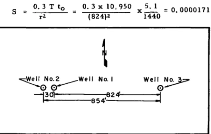
The relative locations of the three wells at Gridley are shown in Figure 6. Well No. 3 was pumped and Wells No. 2 and 1 were used as observation wells. The following analysis is presented from Well No. 1 since more accurate measuring devices were used in that well and wells 1 and 2 were so close together as to make the analysis of Well No. 2 data of relatively small value.
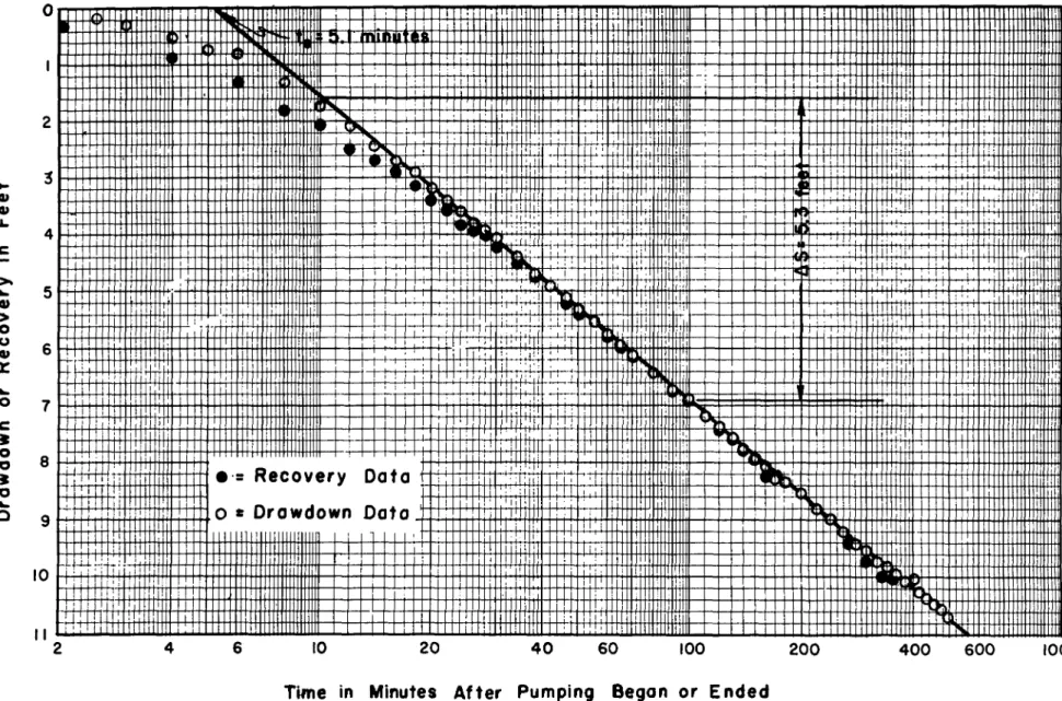
Drawdown Method. The first step of the analysis was to plot the drawdown in Well. 1 versus the elapsed time in minutes after pumping began in Well No. 3, as was done in Figure 5. It can be noted that during the early part of the test, the points indicated a curvature but, as t became larger, the points fell along a straight line. The "slope" (A s) of this line is 5.3 feet per log cycle. The coefficient of transmissibility is determined from equation (IV) as follows:
This straight line, extended back to the line of zero drawdown, indicates a tO of 5.1 minutes, or days. Therefore, the coefficient of storage is computed from equation (V) as follows:
Recovery Method. The formation coefficients T and S may also be determined from the recovery data col-lected during the Gridley test after pumping had ended. The recovery curve is obtained by plotting the amount the water level has raised from the extrapolated draw-down against the elapsed time after pumping ended. It should be noted that the recovery is not measured from the lowest point of drawdown. It is measured from an extended curve of what the water level would have been if the well had continued pumping. This is illustrated in Figure 7. This may be plotted on the same paper as the drawdown curve as was done in Figure 5. If the pumping rate remained exactly constant throughout the pumping period of the test, if the aquifer had been in exact hydraulic equilibrium before pumping began, and if all the assumptions of the nonequilibrium method were exactly true for a particular test, the recovery curve should fall on exactly the same line as the drawdown curve. However, these conditions are rarely completely met in the field and the recovery curve will usually depart slightly from the drawdown curve.
The formation coefficients are determined from the recovery curve in exactly the same way as from the drawdown curve by either the "type curve" method or the modified nonequilibrium method. For the Gridley
19
pumping test the formation coefficients as determined from the recovery data are:
Estimation of Future Pumping and Non-Pumping Water Levels
For estimating water level recessions and interfer-ences due to pumping from the aquifer, averages of the aquifer coefficients as determined from the drawdown and recovery data were used. Thus:
As a hypothetical problem, let it be assumed that the anticipated pumping schedule is to pump the three wells simultaneously for 8 hours per day at 100 gpm each. It is desired to estimate the pumping and non-pumping water levels for each well for the first 10 years of op-eration. For purposes of illustration it will be assumed that all the wells are of the same construction and have the same hydraulic characteristics.
In order to estimate the pumping levels in the wells, three things must be considered.
1.) The drawdown in each well caused by its own pumping.
2.) The interference in each well caused by the other wells pumping.
3.) The areal recession of the water level due to the long-term extraction of water from the aquifer. Self-caused Drawdown. The drawdown in each well caused by its own pumping (assumed to be the same in each well) can be estimated from the drawdown in Well No. 3 during the pumping test. The 8 hour draw-down in Well No. 3 while pumping at 220 gpm was 31.5 feet. An approximate figure for the drawdown while pumping at 100 gpm can be had by multiplying the ratio feet. In making this esti-mate of the drawdown at 100 gpm it was assumed (neg-lecting well loss) that the drawdown was proportional to the pumping rate. That is to say Sw = BQ. A better equation is Sw = BQ + CQ2, where Sw is the drawdown in the well, Q is the pumping rate, and B and C are constants. However, in the absence of a step drawdown test the constants B and C cannot be accurately evaluated. The next best alternative is to use the equation Sw = BQ which would ordinarily give a slightly greater drawdown than the actual when adjusting from a higher pumping rate to a lower one as was done here. Conversely, it would yield a slightly smaller drawdown than would actually occur when adjusting from a lower pumping rate to a higher one. For a better understanding of the factors involved, see the section on the step-drawdown test.
Interference. In estimating the drawdown in each well caused by the pumping of the other wells, it is convenient to construct an interference curve. This is done with the use of Table I and equations (I) and (III)
21
It is desired to calculate the interference at the end of the daily 8 hour schedule in each well caused by the other wells pumping. For this case u =
where r is in feet from a discharging well. Equation (I) becomes:
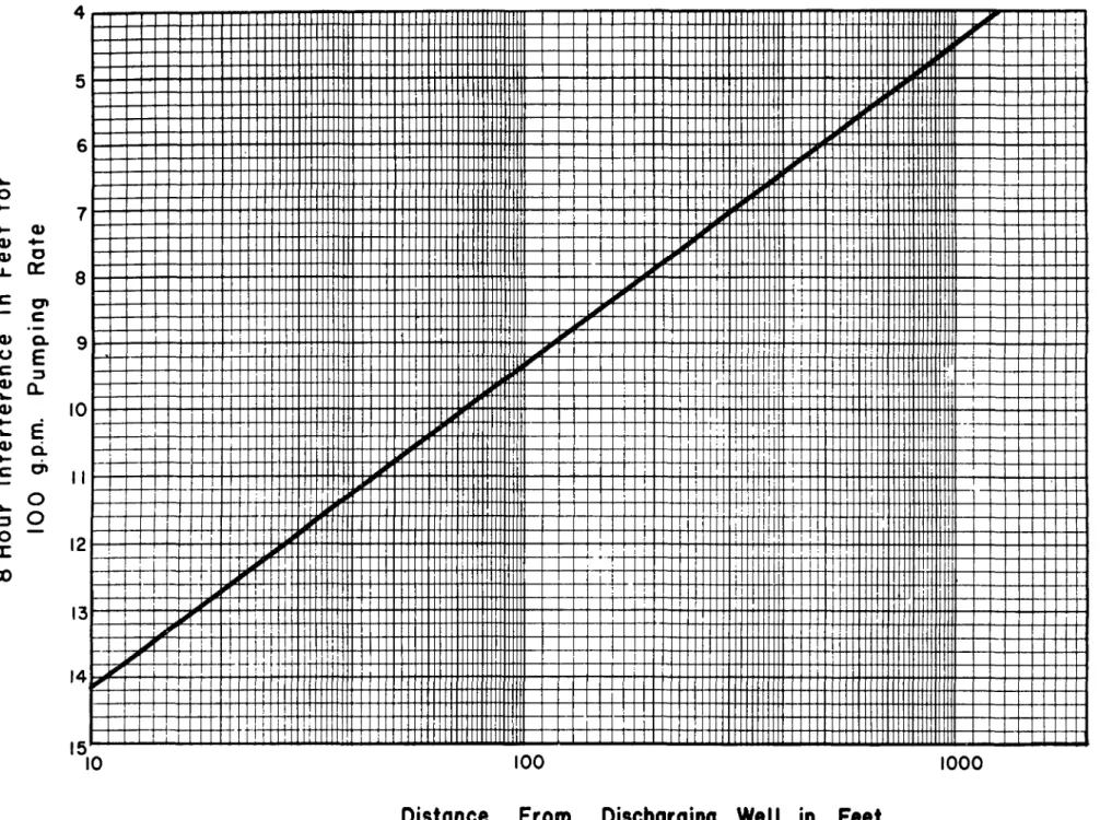
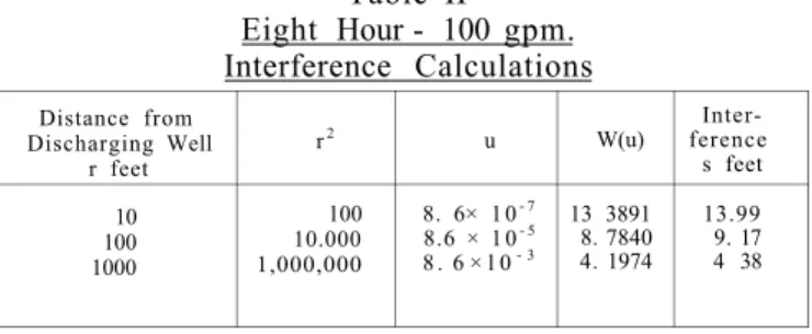
An interference table is then set up as follows: Table II Eight Hour - 100 gpm. Interference Calculations Distance from Discharging Well r feet r 2 u W(u) Inter-ference s feet 10 100 1000 100 10.000 1,000,000 8. 6× 1 0- 7 8.6 × 1 0- 5 8 . 6 × l 0- 3 13 3891 8. 7840 4. 1974 13.99 9. 17 4 38
In Table II. the values of r were selected as multiples of 10 for ease of calculation. The values of u were cal-culated by equation (III). The values of W(u) were ob-tained from Table I for the corresponding values of u. The values of s were then calculated by equation (I).
The interference curve is obtained by plotting r versus s on semi-logarithmic graph paper as shown in Figure 8. For a case where u is less than 0.01, only two val-ues of s need be calculated, for the semi-logarithmic relationship is a straight line. From this interference curve a table of interferences may be compiled show-ing the interference of each well on the others and the total interference in each well (see Table HI). The total drawdown is obtained by adding the self-caused drawdown of 14.3 feet to the total interference of each well. Table III
Interference Between Wells
Eight Hours Pumping At 100 gpm For Each Well Interfering
Well Well No. 1 Well No. 2 Well No. 3
Well No 1 Well No . 2 Well No. 3
Interfering Well Well No. 1 Well No. 2 Well No. 3 Distance between wells in feet Inter-ference in feet Distance between wells in feet Inter-ference in feet Distance between wells in feet Inter-ference in feet Interfering Well Well No. 1 Well No. 2 Well No. 3 30 824 11.85 4.90 30 854 11.85 4.85 824 854 4.90 4.85 Total Inter-ferences in feet Self-caused drawdown 16.75 14.30 16.70 14.30 9.75 14.30 Total draw-down in feet 31.05 31.00 24.05
22
Areal Recession. In order to estimate the areal re-cession of the water level due to the long term extrac-tion of water from the aquifer, an approximaextrac-tion has been used in Illinois for the past 10 years with reasona-ble success. The assumption is made that the long term effect of a total extraction of 300 gpm for 8 hours per day will be the same as that of a continuous extraction of 100 gpm. That is to say: the pumpage is assumed to be spread over the entire day at a proportionately lower rate. This assumption allows a simple approximate solu-tion of an otherwise difficult problem. In addisolu-tion, the recession is calculated for an arbitrary point 1000 feet from the center of pumpage. For this solution, it is not necessary to know where the center of pumpage is lo-cated since the general areal recession of The water level is being estimated. Equations (I) and (III) will be used. For this particular case equation (III) becomes:
and equation (I) becomes:
A recession table is constructed similar to Table IV. Table IV
Areal Recession
In Table IV the values of t were assumed from 1 day to 10 years at arbitrary intervals. The values of u were calculated by equation (III). The values of W(u) were ob-tained from Table I. The values of s were calculated by equation (I). The recession values were obtained by
de-ducting the 1 day drawdown from each value of s. The 1-day drawdown at the 100 gpm rate is deducted from each value of s because the initial drawdown of each well is incorporated in the self-caused drawdown due to its own pumping alone.
The Future Pumping and Non-Pumping Water Levels. From Tables III and IV and the test data sheet, Table V may be constructed.
Table V
Recession Plus Drawdown
Total Drawdown
in feet Recession Plus total drawdown in feet after Total
Drawdown
in feet 1 day 10 days 100 days 1000 days 10 years Well No. 1 31.05 31.05 33.44 35.56 38.23 39.64 Well No. 2 31.00 31.00 33.39 35.51 38.18 39.59 Well No. 3 24.05 24.05 26.44 28.56 31.23 32.64
The decline of the non-pumping water levels and the pumping levels of the three wells is illustrated in Figure 9. By adding the original non-pumping level of any of the three wells to the abscissa of the appropriate point on the recession curve of Figure 9, the non-pumping water level in that well may be estimated for a particular time after the well has been put in service. The pumping water lev-els are estimated by adding the abscissae of the appropri-ate pumping wappropri-ater level curve to the original non-pump-ing water levels.
It should be noted that this is strictly an illustrative example of method and has no relationship to the actual situation at Gridley. Actually Wells No. 1 and 2 at Grid-ley were old wells and were replaced by Well No. 3. The assumption that the aquifer was homogenous and of constant thickness was slightly in error here also. This is indicated by the fact that the estimated self-caused draw-down in Well No. 3 was 14.3 feet while the calculated drawdown in the aquifer 10 feet from the well was 14.11 feet for the same pumping period. This indicates that the aquifer is probably thicker or more permeable in the vicinity of Well No. 3 than it is in the vicinity of Wells No. 1 and 2.
AQUIFER OF LIMITED AREAL EXTENT
The assumption that an aquifer is of infinite areal ex-tent is frequently invalid. Exceptions to this assumption seem most frequent when the aquifer is composed of un-consolidated sands and gravels.
Hydrologic Boundaries
The aquifer may be bounded on one or more sides by impermeable material in the vicinity of a well. Figure 10 is a sketch of a hypothetical aquifer bounded on two sides by impermeable material. While the situation de-picted deals with an artesian formation, similar situations occur for water-table formations.
For this discussion, it is assumed that the aquifer ex-tends for great distances in both directions normal to the cross section shown in Figure 10.
When pumping begins in the pumped well, a region of reduced water pressure is formed around the pumped well. This is called the "cone of depression". The "cone of depression" continues to grow as long as the well is pumped (except where recharge areas may become in-volved). If the aquifer is homogeneous and isotropic, the base of the "cone of depression" is circular and the growth of the radius of that circle has a definite rela-tionship with the elapsed pumping time. This is indicated by both equation (III) and equation (V). As the radius of
24
FIG. 10. HYPOTHETICAL CROSS-SECTION SHOWING AN AQUIFER OF LIMITED AREAL EXTENT
the base of the "cone of depression" grows it passes the observation well and the water level in the observation well begins to lower. As the cone continues to grow, it eventually touches the impermeable boundary to the right of the pumped well. It can no longer grow in that direc-tion.
The behavior of the cone of depression, where there is only one boundary, is conveniently described in terms of the interference of an imaginary well, called an "image well". The image well is considered to be lo-cated twice as far from the pumped well as the imper-meable boundary. A line between the pumped well and the image well is at right-angles to the impermeable boundary. Figure 11 is a cross section of the idealized aquifer (including image well) that would be imagined, for purposes of analysis, to replace the right-hand portion of the situation shown in Figure 10.
The image well is assumed to be pumped at exactly the same rate as the pumped well. Since the formation is homogeneous and isotropic, the cone of depression for the image well touches the boundary at the same time that the acutal cone touches it. From this point on, as pump-ing continues, the effect on the shape of the cone of de-pression of the pumped well is exactly the same as that
of a real well located where the image well is postulated. The cone of depression of the pumped well is conceived of as extending beyond the boundary. Simultaneously, the imaginary cone of depression is conceived to extend beyond the boundary toward the pumped well, thus dou-bling the values of s in the area where the real and im-aginary cones of depression overlap.
As this process continues, the actual cone of depres-sion, modified by the effect of the image well, proceeds toward the left from the boundary toward the pumped well. In the particular situation described, the modified cone reaches first the observation well, and next the pumped well. At the time when the modified cone reaches the observation well, the slope of the recession curve plotted on semi-logarithmic paper doubles. Simi-larly when the modified cone of depression reaches the pumped well, the slope of its "recession curve" doubles.
Figure 11 shows this situation for the right-hand bound-ary in section. For purposes of simplicity, the state of the modified cone prior to its arrival at the observation well is depicted. As the pumping continues, the entire cone of depression shifts downward, and distances " a " and " b " increase.
To complete the analysis of the situation shown in Figure 10, it is assumed the two boundaries are replaced by two image wells which start pumping at the same time and at the same rate of production as the pumped well. The effect of the second image well is similar to that of the first. Figure 12 depicts the type of drawdown curve that would occur in the observation well shown in Figure 10, when two boundaries are present.
Under boundary conditions, the water level in the ob-servation well would remain unchanged for a period of
25
FIG. 12. HYPOTHETICAL SEMI-LOGARITHMIC TIME-DRAWDOWN CURVE ILLUSTRATING THE TYPE OF CURVE OBTAINED WHEN THE AQUIFER IS OF LIMITED AREAL EXTENT
time after pumping begins. When the "cone of depres sion' ' reaches the observation well, the points would begin to curve downward and approach a straight line called the "first limb" of the curve. This "first limb" is the portion of the test from which the aquifer coefficients of transmissibility and storage can be determined by either the "type curve" or modified nonequilibrium method. The points continue down this straight line until they start to bend downward again, approaching the straight line of a ' 'second limb''. This bending downward to the "second limb" is caused by the "cone of depression" being reflected back to the observation well from a boundary, as from the right boundary in Figure 10. The effect is the same as that caused by the imaginary cone of depression from an "image Well" reaching the obser vation well (see Figure 11). It should be noted that the ∆s (change in drawdown per log cycle) is exactly twice as large for the "second limb" as it is for the "first
limb." This is the case because the image well is con ceived to be pumping at the same rate as the pumped well. The "third limb" is caused by the "cone of de pression" reflecting back to the observation well from the left hand boundary (Figure 10). The As of the "third limb" is 3 times as large as for the "first limb". The elapsed time values tO, t1, and t2 are obtained at the
intersection of the "first limb" and the non-pumping level, the intersection of the first and second limb straight lines, and the intersection of the second and third limb straight lines respectively. As indicated in equation (V), the growth of the cone of depression is such that
26 Where:
rO = Distance from pumped well to observation well
r1 = Distance from image well (1) to observation well
r2 = Distance from image well (2) to observation well
K =A constant
Since rO, tO, t1, and t2 of equation (VI) can be de
termined by measurements in the field and from exam ination of Figure 12, it is possible to solve for the dis tances from the observation well to image wells (1) and (2).
If more than one observation well is available, equa tion (VI) may be applied to each observation well and the locations of the "image wells" may be more accur ately determined as to direction. Only rarely are the water level data of the pumped well sufficiently reliable for equation (VI) to be applied to the pumped well. Slight variations in pumping rate usually cause the water level in the pumped well to fluctuate to such an extent that the various "limbs" of a curve of the type in Figure 12 can not be accurately determined. Naturally, if there is no observation well, equation (VI) is not applicable to the pumped well since r is missing. Theoretically it takes three or more wells to which equation (VI) may be applied to locate definitely the positions of the "image wells". If only two wells are available to which equation (VI) may be applied, the position of each "image well" may be narrowed down to one of two possible locations. The impermeable boundaries are known to be half way between the "image wells" and the pumped well.
Example of Analysis. The method of locating first the "image wells" and then the boundaries will be illus trated by a step-by-step analysis of data from a pumping test conducted at Wenona, Illinois. A copy of the pumping test report dated October 14,1947 is included in Appendix II.
The pumping test at Wenona, Illinois was one of the rare cases in which equation (VI) could be applied to the pumped well. Forthatreason it was selected as an exam ple here since it illustrates the application of equation (VI) to an observation well and to a pumped well.
The first step of the analysis is to plot the water level data from the observation well (test well No. 1-47) and the pumped well (well No. 2) on semi-logarithmic graph paper as shown in Figure 13. The three limbs are fitted to the plotted points of each well so that the A s (draw down per log cycle) values are proportioned to a 1:2:3 ratio. For both wells the A s values are as follows:
Limb ∆s 1st 2.65 ft/Log. cycle 2nd 5.30 ft/Log. cycle 3rd 7.95 ft/Log. cycle
For the observation well, tO = 3.7 minutes, t1 =115
minutes, and t2 = 340 minutes. The distance from the
center of the pumped well to the center of the observa tion well is 17.17 feet. By equation (VI),
In the above calculations r01. is the distance from the
observation well to the first "image well" and R02 is the
distance from the observation well to the second "image well".
The same value of K is used for the pumped well as for the observation well.
Equation (VI) applied to the pumped well yields the following results:
The value of r is the distance between the pumped well and the first "image well" and rp2 is the distance
between the pumped well and the second "image well". The next step of the analysis is to plot the possible locations of the "image wells". This was done in Figure 14 by the following method. A suitable scale was chosen and the relative locations of the pumped well and the ob servation well were plotted on a plan. A circle of radius. r01 having its center at the observation well was drawn.
A circle radius of r . with its center at the pumped well was drawn. These two circles should intersect at two points which are the two possible locations of "image
well" No. 1. The two possible locations of the first im permeable boundary are half way between these'' image well" locations and the pumped well. This gives two possible locations for the first impermeable boundary. Unless additional information is available, it is notpos-sible to be sure which of these locations is occupied by the first impermeable boundary. If another observation well were available, the circle drawn from itshould in tersect the circles from this observation well and the pumped well at or near one of the two points of intersec tion shown on Figure 14. This common point of intersec tion would then be the effective location of the first "image well". Frequently some additional knowledge of the geology of the area will aid in the selection of the correct boundary location.
The probable locations of the second "image well" and consequently the second impermeable boundary are found in exactly the same way as for the first image well, except that r02 and rp 2 are used.
27
FIG. 13. SEMI-LOGARITHMIC TIME-DRAWDOWN CURVES OBTAINED DURING A PUMPING TEST AT WENONA, ILLINOIS
It should be emphasized again that in general the water level data obtained from the pumped well is not usable for the location of a boundary. Boundaries are usu ally located by using two or more observation wells. The procedure for each observation well is the same as was illustrated for the observation well in this example. Recharge Boundaries
Another type of aquifer boundary conditions some times encountered in sand and gravel aquifers in Illinois is a surface recharge boundary. This condition exists
when the aquifer has a hydraulic connection with a sur face body of water such as a lake or stream. In this situ ation, the "image well" becomes a well in which water is pumped into the aquifer instead of from it. The time-drawdown curve, instead of bending downward, bends up ward and becomes horizontal after the cone of depression intersects the recharge boundary. Eventually equilibrium conditions are reached and the water levels remain con stant as long as the pumping continues at a constant rate and the surface body of water is able to recharge water to the aquifer as fast as it is being removed. The princi ples used in locating impermeable boundaries are equally applicable to the recharge boundary case.
28
FIG. 14. PLAT SHOWING THE RELATIVE LOCATIONS OF THE WELLS AT WENONA, ILLINOIS AND THE GEOMETRY USED TO LOCATE THE POSSIBLE LOCATIONS OF BOUNDARIES
29
STEP DRAWDOWN TESTS General Discussion
The following theoretical equation defines the draw-down in a pumped well at some particular time after pumping began:
drawdown in the pumped well pumping rate
effective distance from center of well to point of zero drawdown (radius of influence)
physical radius of pumped well
distance from center of well to effective point fn formation where transition from laminar to turbulent flow takes place
laminar flow coefficient of aquifer turbulent flow coefficient of formation gravitational constant
viscosity of the water in the aquifer
A length parameter used in Reynolds number. Probably representative of the pore size in the aquifer.
the density of the water in the aquifer the effective thickness of the aquifer the effective permeability of the aquifer
a coefficient to account for the entrance loss into the well and the turbulent flow of water within the well.
The three components of equation (VII) are illustrated in Figure 15.
Mr. M. I. Rorabaugh* of the U. S. Geological Survey derived a similar equation and published it in December of 1953.( 2 0 )
FIG. 15. CROSS-SECTION OF A WELL SHOWING THE TYPES OF FLOW INVOLVED IN WELL HYDRAULICS
*Credit is due Mr. Rorabaugh for stimulating the State Water Survey work with the step-drawdown analysis through verbal communications with Mr. H. E. Hudson, Jr.
30
Because of the many factors in equation (VII) that cannot be measured, it is not practical for engineering use in its basic form. However, the equation is an aid to understanding the various factors and how they affect the drawdown. Further, if the assumptions made for the non-equilibrium method are valid for a particular case, equation (VII) can be simplified and used conveniently by making one additional assumption. This assumption is that equation (VII), rearranged as follows:
and further simplified to:
yields
and
As a simplification, CQ2 may be taken to represent the well loss. This assumption is not entirely valid be-cause Rt will increase as Q is increased. This actually
makes B and C variables in equation (VIII). However, as B increases, C decreases and if B and C are assumed to be constants, the error in one component of equation (VIII) tends to compensate for the error in the other. Although, the error in one component will not entirely correct the error in the other component, equation (VIII) can be used to obtained fairly reliable values of draw-down over the range of pumping rates generally needed for a particular well.
If it is desired to extrapolate the values of drawdown over a great range of values of pumping rate, the reader is referred to Mr. Rorabaugh'spaper.(20) Mr. Rorabaugh attempts to compensate for the variation in Rt by using the following equation:
in which n is greater than 2. In the opinion of the authors, Mr. Rorabaugh presents the most exact method presently available when a larger range of pumping rates is en-countered but the solution is complicated by the evalua-tion of the three terms B, C, and n. In practice, equaevalua-tion (VIII) has been found to be very useful. More research needs to be done with this type of analysis in order to evaluate accurately the numerous factors involved.
If equation (VIII) is adequate for the range of pumping rates involved, the analysis proceeds as in the following example.
Example of Analysis
The example chosen to illustrate the approximate analysis of the step-drawdown test is a pumping test of
an irrigation well located in the Mississippi River low-lands near Granite City, Illinois.
The pumping test report of the Thomason Irrigation Well No. 1 dated May 21, 1954 gives a brief description of the well (see Appendix II). The well was pumped at three rates, 1000, 1280, and 1400 gallons per minute. The lowest pumping rate was maintained for the longest period in order to determine the recession curve for that pumping rate. The recession curves at the higher pump-ing rates can be estimated from this first recession curve. In the analysis of these data, time was taken into account in a way that would eliminate effects of progressive recession on the data. Values of sw were determined after one hour of pumping at each new rate.
Therefore the estimated slope at 1280 gpm was about 0.269 feet per log cycle and the slope at 1400 gpm was about 0.294 feet per log cycle. These slopes were used to extrapolate each step of the test beyond the period of pumping of each step as shown by the dashed lines in Figure 16. These extrapolations were used to obtain the incremental drawdown caused by a change in pump-ing rate. Before the test was started, the pumppump-ing rate was zero and the water level in the well stood at a constant level. When the pumping test began, the pump-ing rate immediately increased from zero to 1000 gpm. After one hour of pumping the incremental drawdown was 5.43 feet. The pumping rate in this case was con-tinued at 1000 gpm for a total of 100 minutes when the pumping rate was increased to 1280 gpm. One hour after the pumping rate was increased the incremental draw-down caused by the 280 gpm increase was 1.59 feet. The same procedure was followed for each step of the test.
After the one-hour incremental drawdowns were de-termined, these data were arranged in the tabular form shown in Table VI.
Table VI Step-Drawdown Calculations Q . Pumping Rate in gpm 1-hour Incremental drawdown feet sw 1-hour drawdown at pumping rate Q feet sw/ Q feet/gpm 0 1000 1280 1400 0 5.43 1.59 0.72 0 5.43 7.02 7.74 0.00543 0.00550 0.00553
The values of sw and sw/Q were calculated from the first two columns of the Table VI. The values of sw were obtained by adding the incremental drawdown to the sw of the preceding pumping rate. Thus sw at 1000 gpm is equal to 0 + 5.43 = 5.43 and sw at 1280 gpm is equal to
32
5.43 + 1.59 =7.02, etc. After the table was completed,
Sw/Q versus Q were plotted on arithmetic coordinate
paper as shown in Figure 17. A straight line was drawn through the plotted points and extended back to 0 gpm pumping rate. The equation of the form
fits this line. The value of Bis the value of the intercept of the line with the axis and the value of C is the slope of the line. From the line through the points of Figure 17 the following equation was determined.
which is of the form of equation (7) and is the approx imate equation for the drawdown in the Thomason Irrigation Well No. 1 for a pumping period of one hour. Figure 18 shows a plot of this equation and the observed drawdowns for the three pumping rates.
Drawdown equations for longer pumping periods may be determined in the same way. The values of C should not be affected by time, but B should be expected to vary with the logarithm of time.
The well used in this example was a large diameter well in which there was very little turbulent head loss. However, the equation sw - BQ + CQ2 has been found
to work well for wells when the turbulent head losses were much greater. Figures 19 and 20 show the draw down-yield curves for two additional wells where the turbulent losses were greater.
36
COMPLICATING FACTORS The cases given in the foregoing material were chosen
because they were relatively clean-cut and simple, and because they clearly illustrated some of the less-well known basic methods with which groundwater problems are attacked. In many instances, the data from pump ing tests do not lend themselves to precise analysis by the above methods because of interference by factors not encountered in these cases.
The accurate determination of the non-pumping water level is imperative for the methods of analysis described in this report. Whenever possible, all nearby pumping from the aquifer should be discontinued for a period prior to and during the pumping test. The period of shutdown should be of sufficient duration to allow the water level (or pressure) in the aquifer to closely ap proach an equilibrium condition. The time required is usually determined by periodically measuring the water levels in various observation wells after the shutdown. When the water levels in all of the wells have assumed a constant level, the pumping test may be started.
When it is impossible to discontinue all pumping from the aquifer, the pumping of all wells should be controlled and should be kept constant for the period preceding and during the pumping test. The trend of the change in water levels must be determined prior to the start of the pumping test. In this case, all drawdown data must then be determined from the water-level trend curve rather than from single measured non-pump ing levels. The degree of control over all possible interfering pumping from the aquifer has a direct bear ing on the accuracy of the pumping test results.
The section on boundary conditions mentioned the characteristic shape of the drawdown-log time curve that would be expected under recharge conditions. A similar shape may be produced under some instances by transition of the situation in a formation from an artesian condition to a partial or virtually complete water-table condition. Such a change produces a large increase in the coefficient of storage, and actual dewatering of the formation commences sometime after the beginning of the test. A decline in pumping rate may produce a similar curve. A number of cases have been experienced
in which water discharged from the well was not effec tively conducted away from the vicinity of the well, and seeped back into the water-bearing formation, thus producing actual recharge which would not take place under normal operating conditions.
In artesian aquifers, changes in barometric pressure may cause the water level to change. These effects may cause variances in water level as great as one foot. Such variances may be identified if a precise record of variations in barometric pressure is available in the vicinity of the test. Allowance must be made for the fact that such data, obtained from recording barographs located at a distance from the point of test, may have to be adjusted to correct for time lag between the point of barometric pressure measurements and the place of the well test. In addition, since the variation in water level in a well depends on the barometric efficiency of the aquifer, data under non-pumping conditions will be
necessary in order to determine the barometric correc tions to be made. Barometric efficiency may vary from zero under water table conditions to nearly 100 per cent. Similar effects of even greater magnitude occur in wells near streams as a result of stream level fluctuations.(25) In the examples discussed in this report, the data in dicated that the assumption of an isotropic, homogenous formation was valid. In a number of instances, data un affected by other complicating factors gave reason to believe that this assumption was not valid. In some instances the data indicated variances in coefficient of storage as the cone of depression grew. In other cases there were indications that the transmissibility of the formation varied considerably from the vicinity of the well to more remote areas. Where these variations are major, it is clear that a large number of observation wells and a considerable amount of additional test drill ing may be necessary to accurately evaluate the under ground conditions. The application of non-equilibrium methods does not become useless under these conditions: it may be an aid in determining what the actual under ground conditions are and may clearly point out needs for further exploration.
In some instances, alluvial and glacial deposits are found to be highly lenticular, and sometimes have hydrologic interconnections of varying capabilities. In these instances, observation wells may yield misleading or seemingly contradictory results. Cases have also been encountered in which wells have yielded water simul taneously from more than one formation. In these cases, observation wells in any single formation have given non-representative results. Other instances have been encountered in which observation wells have been found to be in a formation completely separate from that con nected to the pumped well.
Misleading results are also obtained from observation wells that are not constructed to be fully open into the pumped formation. An observation well must have permeable connection into the water-yielding formation. The test for this is to pour a quantity of water into the observation well sufficient to raise its level by a readily measureable amount. Timed readings of the water-level change are then taken on the observation well to see how rapidly the water level returns to its original elevation.
For work with the non-equilibrium method, a con stant pumping rate is nearly imperative throughout a major part of each pumping test. If underground con ditions are particularly complex or obscure, an extended period of pumping at a constant rate is important. This extended time of pumping at a constant rate may need to be as long as several weeks, although ordinarily, two or three days will suffice, and in cases known to be un complicated, a few hours may be sufficient.
Gradual changes in pumping rate may have ruinous effect upon drawdown data, and are more to be guarded against than abrupt controlled changes, which may be desirable for step-drawdown analysis of the performance of the well. These controlled changes, however, are
generally of little value in evaluating water-yielding formation characteristics.
Misleading results may also be obtained from partial penetration conditions, under which either the pumped well or the observation well may not be constructed through the full thickness of the formation. Since water bearing formations are frequently stratified, and vertical permeability is generally considerably smaller than hor izontal permeability, partial penetration data may give unreliable results. Methods of correction for partial pen
etration are available in the literature, but these have not
always been found to be entirely satisfactory. For op timum results, the pumped well should substantially pen etrate the water-bearing formation and the observation wells should do likewise. If partial penetration must be present, it should be equal in observation wells and pumped wells.
Especial care must be taken in applying the non-equilibrium method to creviced or cavernous formations.
38
REFERENCES 1. Darcy, Henri, Les Fontaines publiques de la ville
de Dijon, Paris, 1856.
2. Dupuit, Jules, Etudes theoretiques et pratiques sur le mouvement des eaux, Paris, France, 1863. Librarie des Corps Imperiax des Ponts et Chausees et des Mines.
3. Thiem, Gunter, Hydrolische Methoden, J. M. Geb-hardt, Leipzig, 1906.
4. Slichter, C. S., Theoretical Investigation of the Motion of Ground Water, U. S. Geological Survey, 19th Annual Report, 1899, Part 2, p. 360.
5. Turneaure, F. E. and Russell, H. L., Public Water Supplies, John Wiley, third edition, 1924, p. 258. 6. Israelson, O. W. Irrigation Principles and Practices,
New York, John Wiley & Sons, Inc., pp. 189-211, 1950.
7. Wyckoff, R. D., Botset, H. G., and Muskat, M., Flow of Liquids through Porous Media under the Action of Gravity, Physics, Vol. 2, No. 2, pp. 90-113, 1942.
8. Wenzel, L. K., The Thiem Method for Determining Permeability of Water-bearing Materials, U. S. Geol. Survey Water-Supply Paper 679, 1937, pp. 1-57; and Methods for Determining Permeability of Bearing Materials, U. S. Geol. Survey Water-Supply Paper 887, 1942, pp. 83-87.
9. Theis, C. V., The Relation between the Lowering of the Piezometric Surface and the Rate and Dura tion of Discharge of a Well Using Ground Water Storage, Trans, A. G. U., 1935, pp. 519-524. 10. Wenzel, L. K., Methods for Determining Perme
ability of Water-Bearing Materials, U. S. Geol. Survey, Water-Supply Paper 887, 1942, p. 88. 11. Jacob, C. E., On the Flow of Water in An Elastic
Artesian Aquifer, Trans. A. G. U., Part II 1940, p. 582.
12. Wenzel, L. K., and Greenlee, A. L., A Method for Determining Transmissibility and Storage Coef ficients by Tests of Multiple Well Systems, Trans. A. G. U., Part II 1943, pp. 547-560.
13. Cooper, H. H. and Jacob, C. E., A Generalized
Graphical Method for Evaluating Formation Con stants and Summarizing Well-Field History, Trans. A. G. U., Vol. 27, 1946, pp. 526-534.
14. Muskat, M., The Flow of Homogeneous Fluids through Porous Media, McGraw-Hill Book Co., Inc., New York, 1937.
15. Theis, C. V., The Effect of a Well on the Flow of a Nearby Stream, Trans. A. G. U., Part III, 1941, pp. 734-737.
16. Ferris, J. G., Ground-Water Hydraulics as a Geo physical Aid, Michigan Dept. of Conservation, Tech nical Report No. 1, Lansing, Michigan, March 1948. 17. Meinzer, Oscar E., Physics of the
Earth-IX-Hydrol-ogy. McGraw-Hill Book Co., New York and London, 1942.
18. Jacob, C. E., Drawdown Test to Determine Effec tive Radius of Artesian Well. Proc. A. S. C. E., Vol. 72, No. 5 (May, 1946), pp. 629-646.
19. Chow, V. T., On the Determination of Transmis sibility and Storage Coefficients from Pumping Test Data. Trans. A. G. U., Vol 33, No. 3 (June, 1952), pp. 397-404.
20. Rorabaugh, M. I., Graphical and Theoretical Analy sis of Step-Drawdown Test of Artesian Well. Proc. ASCE, Separate No. 362, Vol. 79 (December, 1953). 21. Wisler, C. O. and Brater, E. F . , Hydrology. Chapter
VII, Groundwater by Ferris, John G., John Wiley & Sons, Inc., New York. (1949).
22. Jacob, C. E.f On the Flow of Water in an Elastic
Artesian Aquifer. Transactions, Am. Geophysical Union, pp. 574-586. (1940 Part II).
23. Brown, R. H. Selected Procedures for Analyzing Aquifer Test Data. Journal A.W.W. A., Vol. 45, No. 8 (August 1953), pp. 844-866.
24. Habermeyer, G. C, Public Ground-Water Supplies in Illinois, Illinois State Water Survey Bulletin No. 21, 1925.
25. Suter, Max. Apparent Changes in Water Storage During Floods at Peoria, Illinois. Trans. A. G. U., Vol. 28, No. 3 (June 1947), p. 429.
39
APPENDIX I