Measuring Managerial Ability Using a Two-stage SFA-DEA Approach

(1)

Measuring Managerial Ability Using a

Two-stage SFA-DEA Approach

Stefania Veltri

1

*, Giovanni D

’

Orio

2

and Graziella Bonanno

3

1_{Department of Business Administration and Law, University of Calabria, Arcavacata di Rende, Italy}

2_{Department of Economics, Statistics and Finance, University of Calabria, Arcavacata di Rende, Italy}

3_{Department of Computer, Control, and Management Engineering}_‘_{Antonio Ruberti}_’_{- Sapienza University,}

Rome

Thearticlefocusesonthemeasurementofarelevantcomponentofthehumancapital,themanagerialability(MA). QuantifyingMAiscentraltomanagementliterature.Priorresearchindicatesthatmanagerspeciﬁcfeatures(ability,

talent,reputation,orstyle)affecteconomicoutcomesbut,inmanagementliterature,mostofthemeasures usedin archivalresearchalsoreflectsignificantaspectsofthefirmthatareoutsideofmanagement’scontrol.Thearticleaims tofindameasure,betterthanexistingones,whichallowsdistinguishingtheeffectofthemanagerfromtheeffectof thefirmincreatingfirmvalue.Thearticleusesthe“two-stageSFA-DEA”approach,inwhichbothStochasticFrontier Approach (SFA)andData EnvelopmentAnalysis (DEA)areused toestimatethe efficiencyscoresfirmsadoptto derive ameasureofMA. Theidea istoobtainameasure ofMAas aresidueofthe inefficiencyequationofSFA

andtouseitasanewinputtoinsertinthe“second/third”DEAstage.Italianbankshavebeenchosenasthesample toinvestigateandimplementthemodel.Thedifferencesinresultswithorwithoutthis newMAmeasureprovide evidenceoftheexistenceofthiscontribution.Theoriginalityofthearticleconsistsinthepropositionofanewmodel tomeasureMA,whichoutperformsthealternativemeasures,simpletouseasitisbasedoneasilyobtainableﬁnancial

dataandavailableforabroadcrosssectionofﬁrms,soopeningthedoortoawidearrayofstudiespreviouslydifﬁcult toconduct.

INTRODUCTION

Managing IC efﬁciently (that is, managing and transforming various intangible resources to create or maximize value) is considered the key to sustain competitive edge for each kind of organization (Kujansivu, 2009; Kweh et al., 2013; Veltri & Bronzetti, 2015). The measurement of intellectual capital (IC) and its contribution to theﬁrm’s value is one of the central theme of the IC literature, since from the pioneering article of Bontis (1998) (Andrikopoulos, 2010; Booker et al., 2008; Dumay, 2014; Serenko & Bontis, 2004; Veltri, 2012). Several are the measurement method proposed and used in literature, both quantitative and qualitative (Pulic, 2000; Veltri, 2014). Nonetheless, there is no consen-sus on IC measurement (Dumay, 2014; Uziene, 2010), and many frameworks have been criticized

as they focus on single dimension on IC, without taking into consideration the complex process of IC efﬁciency management, and to be subjective (Feroz et al., 2003). Recently, data envelopment analysis (DEA), a non-parametric approach, has be-come fashionable in the IC management research (e.g. Campisi & Costa, 2008; Kweh et al., 2014a; Lu & Hung, 2011; Lu et al., 2010; Wu et al., 2006; Yang & Chen, 2010), also because DEA allows mul-tiple inputs and mulmul-tiple outputs to be evaluated concurrently without requiring prior information about the relationship among multiple performance measures and interactions among various perfor-mance measures in an objective way (Alfano and D’Orio, 2002).

In this study, the authors also employ DEA to evaluate the IC efﬁciency management, but this study is different from others using DEA to measure IC (Kwehet al., 2013; Leitneret al., 2005; Yalama & Coskun, 2007) for two main reasons. Theﬁrst reason is that the paper do not use just the DEA approach, but a more complex approach, in which both sto-chastic frontier approach (SFA) and DEA are used *Correspondence to: Stefania Veltri, Department of Business

Ad-ministration and Law, University of Calabria, Cubo 3C, Ponte P. Bucci, 87040 Arcavacata di Rende (CS), Italy.

(2)

to estimate theﬁrm’s efﬁciency scores and to derive a measure of the managerial ability (MA).1

The second reason is that the focus of the paper is not on the overall IC, but on a relevant component of the human capital, the MA, and in detail the aim of the paper is to find a measure, better than existing ones, that allows distinguishing the effect of the manager from the effect of thefirm in creating firm value.

Quantifying MA is a central theme for manage-ment literature. Prior research indicates that manager specific features (ability, talent, reputation, or style) affect economic outcomes and are therefore important to economics, finance, accounting, management, and IC research as well as to practice. Prior research is limited to measures such as media coverage and historical returns, which are difficult to attribute solely to the manager versus the firm (Rajgopal 2006), or manager fixed effects, where there is evidence of a manager-specific effect, but the quantifiable effect is limited to managers who switch firms (e.g. Bertrand & Schoar, 2003; Bamberet al., 2010; Geet al., 2011).

The main aim of the paper instead, coherently with Demerijan et al. (2012), is to provide a more precise MA measure than the existing measures (i.e. to exhibit better an economically signiﬁcant manager-speciﬁc component), but at the same time containing less noise than existing proxies of MA.

The paper addresses its aims by applying an approach stemming from the three-stage estimation (Friedet al., 2002) but more sophisticated than this, hereafter “two-stage SFA-DEA” approach. This method consists of estimating the frontier and the inefficiency equation simultaneously at the first stage when SFA is set up. We used the SFA specifi -cation proposed by Battese and Coelli (1995) that allows the constraints of the “two-step” approach to be avoided. In this way, thefirst and the second stages proposed by Fried et al. (2002) are incorpo-rated in a single one, and the efficiency scores are es-timated through a parametric method which takes into account also a random error and not only the inefficiency detracting from the frontier as in DEA.

The idea behind the paper is to obtain an MA mea-sure as a residue of the inefﬁciency equation and to use it as a new input to insert in the second stage when DEA are used. Italian banks have been chosen as the sample to investigate and implement the model, as the banking industry has been the object of several studies employing DEA methodology (Batteseet al., 2000; Casuet al., 2004; Seiford & Zhu, 1999).

The originality of the paper consists in the propo-sition of a new model to measure MA, which out-performs the alternative measures of MA, simple to use as it is based on easily obtainable financial data and available for a broad cross section offirms. We believe that our MA score exhibits an economi-cally significant manager-specific component and contains less noise than existing proxies of MA. This more precise measure of ability opens the door to a wide array of studies that previously were difficult to conduct.

LITERATURE REVIEW

The impact of management on firm performance is a topic of enduring interest in the managerial litera-ture. There are several proxies used in the literature to measure MA. Some studies refer to broader mea-sures to proxy the MA, such as the prior industry-adjusted stock returns (Fee & Hadlock, 2003), the CEO’sfinancial press visibility and thefirm’s prior industry-adjusted return (Rajgopalet al., 2006), and a combination of CEO tenure, prior media men-tions, appointment from outside of the firm, and prior industry-adjusted stock returns (Milbourn, 2003). Other studies (Carter et al., 2010; Tervio, 2008) used executive pay to infer MA. A number of studies proxy MA looking at the market reac-tions, such as Hayes and Schaefer (199), which iden-tify able managers as those who were hired away by anotherfirm, and Bennedsenet al. (2010), which ex-amine firm profitability following the death of a CEO. Several studies,finally, rely on managerfixed effects as measure of CEO ability, such as Bertrand and Schoar (2003), Bamber et al. (2010), and Ge

et al. (2011). Anyway, all of the above examined measures lack precision and often rely on infrequent events.

Studies using DEA are characterized by the aim to provide a more precise measure of MA. Among these, Murthiet al. (1996, 1997) measure MA in the industry sector, Barr and Siems (1997) and Leverty and Grace (2012) within the bank and insurance sec-tors. In each of these studies, the inputs and outputs to the DEA vectors are industry specific. For example, in Murthiet al. (1996) the inputs include product quality and product price, and the outputs include market share. In the Leverty and Grace (2012) insurance study, the inputs include adminis-trative and agent labour, and the outputs include the present value of real losses incurred for personal and commercial short-tail lines. The study of Demerjianet al. (2012), instead, measures efficiency for a large cross section offirms, spanning most in-dustries. In detail, they use as DEA inputfive stock variables (net purchasedfixed assets, net operating leases, net Research & Development, purchased goodwill, and other intangible assets) and twoflow variables (cost of inventory and selling &

1_{A similar approach has been used by Kweh}_{et al}_{. (2014b), aimed}

to examine the relationship between corporate social responsibil-ity (CSR) and corporate performance using a two-stage approach, in thefirst stage evaluating the efficiency and metafrontier frame-work of companies in the US telecommunications industry, then regressing CSR on the efficiency scores in the second stage.

(3)

administrative expenses) to capture the choices managers make in generating revenues (output). Demerjianet al.’s (2012) study also differs from the others because the authors modify the DEA gener-ated firm efficiency measure by excluding from it keyfirm-specific characteristics that the authors ex-pect to aid (firm size, market share, positive free cash flow, and firm age) or hinder management’s efforts (complex multi-segment and international operations), attributing the unexplained portion of firm efficiency to management. The paper proposes an MA measure that, coherently with Demerjian

et al. (2012) allows distinguishing the effect of the manager from the effect of the ﬁrm and to obtain an ordinal ranking of quality for the sampledﬁrms using a“two-stage SFA-DEA” approach described in the following section.

As IC is considered“firm-specific”and “context-specific”from the third stage IC researchers (Dumay, 2014; Guthrieet al., 2012),2 _{we decided to apply the}

model to a specific industry, the banking sector, and to a defined context, the Italian context, one of the largest European markets (Casuet al., 2004). Manag-ing IC within the service sector is particularly rele-vant (Bowen & Ford, 2002), and an IC approach is particularly relevant in a peculiar service sector such as banking sector, for the significance that IC play in such industry (Curadoet al., 2014).

Moreover, to use of the “two-stage SFA-DEA” approach make essential to choice of a sample of firms within the same business sector, asfirms have to be comparable to presume that the processes that transform tangible and intangible inputs into value within afirm are similar.

Several studies employing efﬁciency methodol-ogy (DEA or SFA) focused on the banking sector (Avkiran, 2011; Battese et al., 2000; Casu et al., 2004; Deville, 2009; Devilleet al., 2014; Halkos & Salamouris, 2004; Kao & Liu, 2014; Matthews, 2013; Seiford & Zhu, 1999; Wang et al., 2014; Yalama & Coskun, 2007), also in Italy (Aiello & Bonanno, 2013, 2016a, 2016b; Bonanno, 2014). Nevertheless, to date, no study uses a two-stage SFA-DEA approach to measure MA in banking sector.

THE“TWO-STAGE SFA-DEA”APPROACH

DEA is a highly sophisticated method of evaluating and measuring organizational performance. It

allows to measure the relative productive effi -ciency of each member of a set of comparable or-ganizational units (DMUs) based on a theoretical optimal performance for each organization. DEA evaluates the relative efficiencies of DMUs with-out making any assumptions abwith-out the functional relationship between inputs and outputs in these units, and this is its strongest point and the rea-son why DEA could be considered a new, more suitable approach to evaluate the productivity of intangible resources, hard to identify and to model (Campisi & Costa, 2008). In the DEA, the technical DMU efficiency is defined with regards to the other DMUs of the sample, with some units lying on the efficiency frontier (efficiency measure equal 1), some others below efficiency frontier (effi -ciency measure<1).

Nevertheless, this approach is by no means with-out limitations. One of the main limitations attrib-uted to the method is that units could be below the efﬁciency frontier exclusively for inefﬁciency reasons.

To overcome this limit, some researchers prefer to complement DEA with the method called stochastic frontier approach (SFA). In detail, SFA is a paramet-ric method which allows inference to be made on the estimated parameters by assigning a distribu-tion funcdistribu-tion to the error. Further classification distinguishes the stochastic methods from the deter-ministic ones. The former takes into account that a unit may stray from the efficient frontier also owing to reasons of a random nature and not only to inefficiency.

The main advantage of SFA is due to the possi-bility of breaking down the error in two parts, the inefficiency and the random errors. Under this profile, SFA is preferable to the Data Envelopment Analysis (DEA), which supposes that the distance from the frontier is explained entirely by ineffi -ciency and it does not consider random errors such as maybe, variables measurement errors, or those due to unexpected events. A further advan-tage of the SFA method is the possibility of inserting a set of variables in the model that explain the inefficient component. In this way, SFA method offers the guarantee to consider an exogenous component of inefficiency in the estimation of the frontier.

The methodology used by Friedet al. (2002) is one of the most widely applied in studies keen to use DEA overcoming its main limitation. The Fried

et al.’s methodology consists of three steps: in the first one the authors use DEA in order to estimate the initial measure offirm performance; in the sec-ond stage, the first-stage performance measures are regressed against a set of variables; in this way, a decomposition of the variation in the performance is obtained, which is formed of a part attributable to environmental effects, a part due to managerial inef-ficiency, and a part attributable to random errors;

2_{Originally, Petty and Guthrie (2000) outlined two stages}

associ-ated with developing IC as a researchﬁeld. In theﬁrst stage (from the late 1980s to the early 1990s), efforts focused on raising aware-ness of IC and understanding its potential for creating and man-aging a sustainable competitive advantage. The second stage of IC research (from the late 1990s to the early 2000s) dealt mainly with the process of measuring and managing IC from a top-down perspective. Guthrieet al. (2012) extended Petty and Guthrie’s study to introduce a third stage in IC research (from 2004 until now), focused on a critical examination of IC in practice (Veltri & Bronzetti, 2015).

(4)

finally, in the third step, DEA is used in order to re-evaluate thefirm performance with adjusted inputs (or outputs, depending on the orientation of first stage DEA).

The methodology used in this work is an alterna-tive to the three-stage DEA SFA approach proposed by Fried et al. (2002), in which we implement the specification proposed by Battese and Coelli (1995), which allows to estimate the frontier model and the inefficiency equation in a simultaneous way. In this way, the first and the second stages shown by Fried et al. (2002) are incorporated in a single one, and we estimate the efficiency scores through a parametric method which, among other things, takes into account also a random error and not only the inefficiency detracting from the frontier as in DEA. Our idea is to obtain an MA measure as a residue of the inefficiency equation and to use it as a new input to insert in the second stage when DEA is set up. For these reasons, it would be appropriate to call the methodology used in this study“two-stage SFA-DEA”.

In particular, the methodology used in this work can be described as follows:

1. The first stage involves estimating simulta-neously the cost frontier and the inefficiency equation defined in the system (1):

Costit¼C y� it;wit�þuitþvit uit¼X K k¼1 ηkzitkþeit 8 > > > > < > > > > : (1)

where Costitis the logarithm of total cost incurred by thei-th bank at time t; yit represents the vector of outputs obtained from the bankiin yeart;witis

the vector of input prices;βjandγnare the respective parameters to be estimated;uitis an erratic compo-nent that measures the inefficiency and is a non-negative variable;vitis, instead, the random error. Moreover,zitrepresents the vector of variables that influence thei-thbank. Our interest is to obtain the MA measure as residues of the inefficiency equation and to introduce it in the DEA second stage estimation.

2. The second stage consists in implementing the DEA approach with another input, the MA esti-mated in the previous step. DEA is the most used non-parametric method in the literature of MA (Demerjian et al., 2012; Hajiha & Ghilavi, 2012; Leverty & Grace, 2012).

Letxiandqibe, respectively, the column vectors of inputs and outputs,Xand Qthe input matrix and the output matrix, the variable returns to scale (VRS) linear programming problem can be written as follows (Afriat, 1972; Bankeret al., 1984; Battese

et al., 2005): minθ;λ θ; st �q_iþQλ≥0; θxi�Xλ≥0; I1’λ_¼1 λ≥0 (2)

whereθis a scalar,λis aI× 1 vector of constants and the third expression of (2) is the convexity constraint.

THE SAMPLE: DATA AND VARIABLES

Data are from the ABI Banking Data, which pro-vides the balance sheets of Italian banks from 1993 to the present. Moreover, some variables (for exam-ple, bad loans calculated by geographical location of customers) are taken from the BIP (“Base Informativa Pubblica”online) released by the Bank of Italy. The period covered by this analysis is 2006–2011. There were 686 banks in 2006, 692 in 2007, 689 in 2008, 686 in 2009, 648 in 2010, and 631 in the last year. The sample consists of mutual-cooperative banks, henceforth MCBs (on average 63%), Ltd (on average 32%), and Popolari banks (on average 6%). As can be seen, most of the banks are small and minor (92% of the sample in 2006 and 94% in 2011). In addition, the proportion of banks that have their main office in the North is 60% of the sample. This is a much higher value than that for banks that have their main office in the South (20%). In order to highlight some information about the Italian Banking System, Table 1 reports the distribution of Total Assets for geographical areas and legal categories. As can be seen, this industry is characterized by a breakdown and, for each macro-area or legal class, banks have specific and different characteristics.

With regard to the variables used in the econo-metric analysis, in the extensive review proposed by Berger and Humphrey (1997), it is argued that the intermediation approach proposed by Sealey and Lindley (1977) is the most appropriate to evalu-ate ﬁnancial institutions. For these reasons, the variables we include in the model are selected according to this approach.

Although there is a heated debate about which speciﬁcations of inputs and outputs to choose in the study of bank performance, there is a certain consensus in considering loans to customers (y1) as

the main banking output. We introduce another out-put into the model, namely the non-interest income (y2). This choice is justiﬁed by the fact that banks

nowadays offer a range of non-traditional “collat-eral”services for which they obtain positive gains. The third output used in this work is that of securi-ties (y3), composed of loans to other banks, equities,

(5)

we use labour, capital, and deposits. In the ﬁrst stage, we use the input prices in order to estimate the cost frontier, while in the second stage, we apply a production frontier introducing a fourth input given by the MA measure derived in theﬁrst stage. There are three traditional inputs: labour (x1) is

mea-sured as the number of employees of individual banks; the cost of labour (w1) is calculated as the

ratio of personnel expenses to the number of employees; the cost of capital (w2) is measured in

this work as the ratio of expenses that are not consid-ered in the other input variables in the frontier model and the banking product (x2). Therefore, the

numer-ator includes administrative expenses (excluding personnel expenses), operating expenses, the interest expense net of interest on amounts due to customers, depreciation of ﬁxed assets, and commission ex-penses. The administrative expenses include cost items, such as those relating to electricity, rent, and maintenance of various types (for details, see Aiello & Bonanno, 2013). Finally, the third input considered is given by the deposits from customers (x3) whose

cost (w3) is given by the ratio of interest paid to

cus-tomers and the total amount of deposits. The depen-dent variable in the cost function, Cost(y,w), is the total cost of individual banks, and this is calculated as the sum of administrative expenses, interest expense, operating expenses, commission expenses, and depreciation ofﬁxed assets.

As already mentioned, the specification made by Battese and Coelli (1995), which allows the simulta-neous estimation of equations of system (1), implies a need to define the determinants of ineffi -ciency. One environmental variable that explains bank performance is credit quality (z1), which we

calculate as the ratio of non-performing loans to total loans to customers. Both these variables are deﬁned by customers’ geographical location and are taken from the BIP of the Bank of Italy. The values of the loans quality (z1) are linked to each

observa-tion through the deﬁnition of four geographical

macro-areas (Bonanno, 2014). In order to take into account the bank’s risk position and the effect that this may have on efﬁciency scores, an indicator of bank solvency (z2) is introduced. This is calculated

as the ratio between regulatory capital and risk-weighted assets and is a measure of banks’capital adequacy in relation to the credit risk. Furthermore, this is calculated on a territorial level by considering the same four macro-areas used for z1. It is also

use-ful to consider the weight of each bank within the in-dustry and, in this sense, the Herfindahl index (z₃), has been adopted. For each geographical macro-area, it is calculated as the sum of the squared mar-ket share of each bank in the sample. This is an issue which has been addressed in many works (Casu & Girardone, 2009; Dongiliet al., 2008; Fontani & Vitali, 2007), which have aimed at verifying whether a higher concentration in the industry, such as has oc-curred in the Italian banking sector since the 1990s, can influence bank efficiency. In general, the out-come is uncertain, since the operations of consolida-tion have resulted in an increase in size with an eye to probable and expected increases in efficiency levels. On the other hand, this may cause an increase in banks market power. Turati (2008) pro-poses a model that captures the relationship between profitability and efficiency. The results sup-port the idea of a competitive banking sector and, ac-cording to the author, the consolidation operations lead to an increase in banks’ bargaining power, which is bad for customers. Theftseindex (z4) is

in-troduced into the model in order to capture the rela-tionship between the effects of the current crisis, reflected in Stock Exchange transactions, and bank efficiency (Bonanno, 2014). Moreover, a dummy for each year of the analysed period is introduced in or-der to consior-der a time effect on the efficiency scores. This dummy is meant to capture what happened in the years before and after the crisis, which reflects phenomena which are different from those gauged by the otherz-variables. Finally, we have included

Table 1 Average values of Total Assets by geographic area and legal category (constant values in mln of euros—NIC Index Istat, base year = 1995)

2006 2007 2008 2009 2010 2011

Banks Total

Assets Banks AssetsTotal Banks AssetsTotal Banks AssetsTotal Banks AssetsTotal Banks AssetsTotal

Geographical area North-West 151 6011 149 6955 144 8210 152 7464 138 5762 129 6370 North-East 241 1636 242 1884 242 1877 239 2045 231 2883 230 3020 Centre 151 3250 150 3106 154 3238 150 3381 144 3182 139 3418 South 143 725 151 701 149 712 145 768 135 742 133 736 Legal category LTD 218 7327 218 7845 222 8593 233 8082 207 8001 193 8879 MCB 431 241 436 257 428 278 414 301 406 318 404 328 POP 37 5276 39 6368 39 5506 39 6001 35 6689 34 7154 Total 686 2764 692 2983 689 3253 686 3268 648 3177 631 3312

(6)

some dummy variables in order to take into account the fact that any difference in the levels of cost efﬁciency may be determined by legal category, geo-graphical location, and/or size of banks.

MAIN FINDINGS

In this section are reported the results of both the stages.

First stage: results from SFA

The translog cost function for the banking sector is estimated as a system of equations. The aspects of the firm’s behavior that we observe are total cost, the allocation of total cost across the various inputs (i.e. input expenditure shares), the firm’s output level, and the input prices that thefirm faces. The translog function allows for both positive and nega-tive scale effects, that is, average cost can both de-crease and inde-crease across the range of the cost function. Moreover, the translog function is more flexible than the Cobb–Douglas form. The elasticity of cost with respect to output is the ratio of marginal to average cost.

Essentially, this allows the observable informa-tion about the behaviour of the ﬁrm such as total resources expenditures, the distribution of these expenditures across inputs, the output yielded by these expenditures, and the resources prices faced by the ﬁrm all to be used in the estimation of the parameters of the model.

In Table 2, there is the estimation of the cost fron-tier for the Italian banking system over the period

2006–2011. All the coefﬁcients of our model for the translog cost function are signiﬁcant.

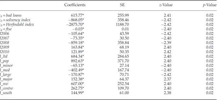
Table 3 shows the cost inefficiency equation for the Italian Banking system (2006–2011). All the coef-ficients are significant. It is worth noticing that the coefficient for“Bad Loans”has a positive sign. This means that the higher the incidence of suffering (or, in other words the lower the credit quality of the ter-ritorial area where the bank has its main office), the higher are the values for estimated inefficiency.

The coefﬁcient of the “Solvency Ratio” has, instead, a negative sign. If banks have high solvency ratio, the lower the risk to which they are subject the lower the level of inefﬁciency that they register.

Interesting information is also provided by the coefficient of Herfindhal’s index that has a negative sign. This means that Banks in which the concentra-tion of Total Assets (relatively to their main office) is higher reached the highest levels of efficiency.

Another aspect to be highlighted is that the coefﬁ -cient of FTSE index has a negative sign. This signals a pro-cyclical trend in efﬁciency.

The highest cost efficiency values are achieved by MCBs and by Banks with the main office in North-East. The efficiency levels are higher in small Banks than in major ones, but minor, medium, and large Banks achieve cost efficiency levels higher than the small ones.3

These results are quite interesting and sometimes surprising such as the one that smaller banks are more efﬁcient than bigger banks (Aiello & Bonanno, 2013; Bonanno, 2014), but for our aim the most

Table 2 Estimates for the cost frontier of Italian banks (2006–2011)

Coefﬁcients SE z-Value p-Value Coefﬁcients SE z-Value p-Value β0 �5.44*** 0.580 �9.38 0 γ11 �0.05*** 0.015 �5.94 0 β1 0.73*** 0.005 14.96 0 γ12 �0.004 0.024 �0.35 0.72 β2 �0.20*** 0.059 �3.32 0 γ22 0.05*** 0.012 8.06 0 β3 0.38*** 0.056 6.92 0 α11 �0.06*** 0.006 �9.20 0 γ1 1.60*** 0.124 12.91 0 α12 0.07*** 0.008 8.58 0 γ2 0.03 0.099 0.35 0.72 α13 �0.02* 0.008 �2.39 0.02 β11 0.04*** 0.002 42.74 0 α21 0.07*** 0.004 14.02 0 β12 �0.06*** 0.006 �21.08 0 α22 �0.05*** 0.008 �6.67 0 β13 �0.03*** 0.006 �10.84 0 α23 �0.002*** 0.007 �0.37 0 β22 0.03*** 0.004 12.40 0 β23 0.02*** 0.007 4.68 0 Sigma2 _119.43* _49.68 _2.40 _0.02 β33 0.01*** 0.004 3.82 0 Gamma 0.9997*** 0.0001 7805.44 0 Log-likelihood 363.15

Source: Own elaboration on ABI data. Signiﬁcance levels:

***= 0.001; **= 0.01; *= 0.05. sigma2₌_σ2

u+σ2v; this is composed of the error variance, given by the sum of the variances of the two components.

gamma =σ2u/σ2; the zero value of this parameter indicates that deviations from the frontier are only due to random error, while values

close to one of the range entail that the distance from the border is due to inefﬁciency. This parameter, in the technique of Jondrow

et al. (1982), is used to separate the component of inefﬁciency (JLMS technique).

3_{In this estimation, BCCs are the group of control for the legal}

cat-egory. Banks that have the main ofﬁce in North-Eastern Italy are the group of control for the geographical side.

(7)

important issue is the following one. We obtain that the erratic componentuit, the share of the composite error that measures inefficiency, has been“cleaned up” from some sources of inefficiency (bad loans, solvency, etc.), then we can use the residual of the inefficiency equation as an acceptable proxy to signal MA.

Second stage: results from DEA

In the second stage, we apply DEA under the hypotheses of both Constant Return to Scale (CRS) and Variable Return to Scale (VRS). The assumption of VRS seems to explain better some features of the organization studied, but it is useful to conduct a

CRS and a VRS DEA upon the same data since doing it this way allows us to decompose the techni-cal efficiency (TE) scores obtained into two compo-nents, one due to scale inefficiency and one due to “pure”technical inefficiency (i.e. wrong input mix or managerial inefficiency). If we have a difference between the two TE scores for a specific observation (or Decision Making Unit) this indicates that the Decision Making Unit has scale inefficiency. When this happens, we can calculate this inefficiency using the difference between the VRS TE score and the CRS TE score.4

4_{The result of the two tests (one for CRS, one for VRS) is available}

on request (in the case of CRS, thet-statistic is equal to 29.10, while in the case of VRS, it is equal to 25.58).

Table 4 Estimated DEA for the Full Sample with and without MA’s measure as new input of the production function

2006 2007 2008

CRS VRS CRS VRS CRS VRS

Full sample—no MA as input 0.9004 0.9090 0.8980 0.9076 0.9000 0.9087

0.0400 0.0434 0.0387 0.0436 0.0393 0.0431

Full sample—MA as input 0.9064 0.9133 0.9096 0.9161 0.9174 0.9230

0.0411 0.0443 0.0417 0.0456 0.0430 0.0457

Nr.of observations 475 495 525

2009 2010 2011

CRS VRS CRS VRS CRS VRS

Full sample—no MA as input 0.8980 0.9070 0.8887 0.8974 0.8943 0.9048

0.0357 0.0401 0.0366 0.0410 0.0368 0.0406

Full sample—MA as input 0.9093 0.9157 0.8994 0.9062 0.8997 0.9082

0.0383 0.0418 0.0394 0.0421 0.0367 0.0403

Nr.of observations 500 472 481

Source: Own elaboration on ABI data.

Table 3 Inefﬁciency equation estimates for Italian banks (2006–2011)

Coefﬁcients SE z-Value p-Value

z1=bad loans 615.77* 255.99 2.41 0.02

z2=solvency index �868.05* 358.46 �2.42 0.02

z3=Herﬁndahl index �2875.70* 1188.70 �2.42 0.02

z4=ftse �0.03* 0.01 �2.40 0.02 d2006 �105.64* 43.59 �2.42 0.02 d2007 �73.35* 30.50 �2.40 0.02 d2008 �859.18* 358.84 �2.39 0.02 d2009 163.84* 68.19 2.40 0.02 d2010 121.89* 50.35 2.42 0.02 d_ltd 684.34* 284.65 2.40 0.02 d_pop 892.63* 371.70 2.40 0.02 d_minor �65.13* 27.14 �2.40 0.02 d_med �402.49* 167.74 �2.40 0.02 d_large �170.87* 70.71 �2.42 0.02 d_major 152.38* 64.37 2.37 0.02 d_nw 607.00* 252.54 2.40 0.02 d_centre 262.75* 109.70 2.40 0.02 d_south 144.99* 61.00 2.38 0.02 Signiﬁcance levels: ***= 0.001; **= 0.01; *= 0.05.

(8)

In Table 4, there are the efﬁciency scores esti-mated with DEA without and with the MA mea-sure as new input of the production function. The standard errors are in italics. We performed a test on the differences between means, and we widely reject the null hypotheses of equality. This result allows us to consider the MA as a signiﬁcant variable to be introduced in the esti-mate of a production function with the DEA approach.

The average efficiency scores of Table 4 show that when we consider the additional input of MA the efficiency results improve. This happens for all the years and for all the observations. The magnitude of improvement is different in different years. Figure 1 shows the trend in the estimated average Efficiency Score. It is clear from the figure that including MA as an input gives us better scores. It means that MA has a positive impact on the effi -ciency of the sample. The trend is increasing from 2006 until 2008, it decreases in 2009 and 2010, and slightly improves for 2011.

In Figure 2, we can observe the magnitude of improvement given by MA. This value is calculated as the differences between the efﬁciency score obtained without this input and the efﬁciency score obtained including in the estimation the proxy of MA.

Figure 1 Trend in the average estimated DEA—full sample with and without MA’s measure (VRS)

Figure 2 Impact of MA (full sample)

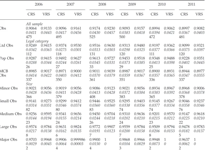
Table 5 Estimated DEA efﬁciency scores of with MA’s measure as input—Full sample—Legal Category—Size

2006 2007 2008 2009 2010 2011 CRS VRS CRS VRS CRS VRS CRS VRS CRS VRS CRS VRS All sample Obs 0.9064 0.9133 0.9096 0.9161 0.9174 0.9230 0.9093 0.9157 0.8994 0.9062 0.8997 0.9082 0.0411 0.0443 0.0417 0.0456 0.0430 0.0457 0.0383 0.0418 0.0394 0.0421 0.0367 0.0403 475 495 525 500 472 481 Legal category Ltd Obs 0.9249 0.9415 0.9374 0.9530 0.9516 0.9630 0.9313 0.9480 0.9197 0.9362 0.9099 0.9321 0.0342 0.0363 0.0275 0.0301 0.0313 0.0303 0.0298 0.0325 0.0377 0.0366 0.0375 0.0397 112 118 131 120 111 120 Pop Obs 0.9287 0.9415 0.9492 0.9627 0.9613 0.9727 0.9453 0.9518 0.9348 0.9488 0.9228 0.9351 0.0288 0.0344 0.0244 0.0261 0.0345 0.0331 0.0373 0.0385 0.0413 0.0398 0.0402 0.0445 26 27 33 29 25 24 MCB Obs 0.8985 0.9017 0.8971 0.90000.0414 0.0422 0.0403 0.0412 0.9011 0.9039 0.8987 0.9017 0.8900 0.8931 0.8944 0.89770.0370 0.0379 0.0359 0.0367 0.0357 0.0365 0.0347 0.0355 337 350 361 351 336 337 Size Minor Obs 0.9021 0.9056 0.9019 0.9056 0.9086 0.9123 0.9021 0.9056 0.8934 0.8967 0.8968 0.9006 0.0428 0.0436 0.0411 0.0428 0.0413 0.0428 0.0372 0.0384 0.0383 0.0392 0.0368 0.0378 366 379 408 383 365 378 Small Obs 0.9141 0.9273 0.9299 0.9412 0.9446 0.9525 0.9295 0.9403 0.9145 0.9267 0.9046 0.9237 0.0314 0.0351 0.0346 0.0374 0.0360 0.0360 0.0338 0.0356 0.0377 0.0334 0.0358 0.0346 82 80 83 74 74 76 Medium Obs 0.9256 0.9595 0.9341 0.9656 0.9450 0.9704 0.9310 0.9636 0.9201 0.9570 0.9147 0.9618 0.0144 0.0194 0.0155 0.0214 0.0244 0.0218 0.0202 0.0210 0.0215 0.0212 0.0225 0.0210 23 24 26 24 23 22 Large Obs 0.9574 0.9784 0.9631 0.9824 0.9772 0.9907 0.9559 0.9784 0.9509 0.9794 0.9478 0.9783 0.0217 0.0138 0.0162 0.0135 0.0191 0.0123 0.0200 0.0158 0.0206 0.0153 0.0182 0.0137 8 6 7 7 8 5 Major Obs 0.9703 0.9968 0.9906 0.999986 0.9900 1 0.9868 0.9966 0.9948 1 0.9637 1 0.0029 0.0045 0.0064 0.00003 0.0150 0 0.0104 0.0029 0.0073 0 0.0062 0 2 4 4 3 2 2

(9)

The highest value is observed in 2008; years 2007, 2009, and 2010 show a similar value of the impact of MA on efﬁciency while the minimum is observed in year 2011.

In particular, when we consider MA as input, in 2008 in which the financial crisis was registered, we obtain an increase in the average effi_ciency. This can clarify the importance of considering this variable. Evidently, a part of efficiency explained by MA positively contributes also in the case of crisis.

Table 5 reports the estimated efﬁciency when we introduce the MA measure as input. We show the results disaggregated for legal category and size. Also, in this table, the standard errors are in italics.5

As can be seen, in the case of VRS, we obtain an increase of estimated efficiencies, but trends remain substantially unchanged. When we disaggregate for legal category, wefind that Popolari Banks perform better than Ltds and MCBs and that the latter regis-ter the worst results. As regards the size, it easy to realize that the largest Banks achieve the higher levels and that with decreasing size also the esti-mated values decrease. These results confi_{rm the} existence of a strong heterogeneity within the Italian Banking System.

We are able to reproduce Table 5 when estimat-ing a stochastic cost frontier in the first stage. We chose not to include it because it does not corre-spond to the focus of the paper. However, on the SF cost side, CCBs perform better than the others one, while Ltds are placed in the same intermedi-ate position with respect to what happens when estimating the production function through DEA. Regarding the size, we find a conflicting result because in this case we obtain that the minor banks are positioned infirst place with the highest levels of cost efficiency, whereas the major banks

are in last place. The ranking remains unchanged with respect to the other banks (small, medium, and large).

CONCLUSIONS AND FUTURE RESEARCH DIRECTIONS

The article focuses on the measurement of a relevant component of the human capital, the MA, and the paper aims tofind a measure, better than existing ones, that allows distinguishing the effect of the manager from the effect of thefirm in creatingfirm value.

Quantifying MA is central to management litera-ture. Most of the measures used in the literature re-flect significant aspects of thefirm that are outside of management’s control. The originality of the pa-per consists in the proposition of a new model to measure MA, which outperforms the alternative measures of MA, simple to use, and based on easily obtainablefinancial data and available for a broad cross section of firms. The paper aims to exploit the possibility of measuring the impact of MA on technical efficiency.

To do this, we use a sophisticated approach to the classical three-stage estimation, in which both Data Envelopment Analysis and Stochastic Frontier Ap-proach are used to estimate the firm’s efficiency scores. This allows us to derive a measure of MA. The method used is a “two-stage SFA-DEA” ap-proach. Our measure of MA is the “clean”part of the residue of the inefficiency equation of Stochastic Frontier Approach, and we use it as a new input in

the “second/third” Data Envelopment Analysis

stage. We observed an improvement in efficiency scores calculated with this new input for all years and for all the average samples. This can be seen as a proxy of positive impact of MA on technical ef-ficiency. We believe that our proxy of MA score ex-hibits an economically significant manager-specific component and contains less noise than existing proxies of MA. This more precise measure of ability allows a wide array of studies that previously were difficult to conduct.

An interesting topic for further research can be to develop a “behaviour”model for inefficient firms. Since we estimate a technical efficiency frontier, the Observations (Decision Making Units—DMU) on the Frontier can be seen as“fashionable”DMU for all the DMU that are not fully efficient (not on the Frontier). In this way, all the frontier DMU can be treated as“peer”. “Peers” define the relevant part of the production frontier for a DMU. If a DMU is not fully efficient, given the previous and following estimation, we can calculate which is the target (i.e. produced output given the used inputs) that the DMU could aim at, if efficient. An example will make it clear (see Figure 3). Output Z can be pro-duced using two inputs y and x. The points on the

5_{In this stage, we exclude banks that register SFA-efﬁciency}

scores with a standard deviation greater than 0.10 between 2006 and 2011 (27 observations). Moreover, DEA requests a full matrix of values; therefore, theﬁnal number of observations, for this step, is 2948.

(10)

iso-product curve (A, C, E, and F—let us not con-sider D yet) are DMUs producing the quantity Z of output in an efficient way, using different technolo-gies (the vectors departing from the origin indicate the input combinations). DMU B produces the quantity Z using a sub-optimal technology. If DMUs on the frontier have a Technical Efficiency score of 1, B will have a smaller Technical Efficiency score, i.e. 0.8. This means that for that DMU could be possible to reduce the consumption of all inputs by 20% without reducing output. If we draw a vector be-tween the origin of the axis and B, the vector will cross the production frontier at the point D. D can be seen as an idealfirm that uses the same technol-ogy of B but efficiently (it uses less inputs for the same quantity of output). D could befirm B using its technology efficiently. Point D can be obtained as a linear combination of point A and C. A and C will be the“peers”firms of B.

Since we can have a proxy of MA as an input (and for all inputs), we can calculate a“weight”for each peer and for each input, and also for MA. The weight obtained for each input, in each estimate and for each“peer”is“the importance”of thatﬁrm as a peer in the linear combination (i.e. in the exam-ple D is at the same distance between A and C so the weight of these two peers will be, i.e. 0.5 and 0.5. If D was very close to A, the weight would be 0.90 for A and 0.10 for C).

Our approach can give some useful direction to non-efficient DMU in the changes needed in each in-put (including MA) to achieve full efficiency, and this can be an interesting starting point for a new work. The idea emerging also from the Figure 3 is that the management can read our empirical results in the direction of reducing thefirm inputs without reducing its outputs or increasing the outputs with the same level of inputs. It is a useful tool to address the managerial decisions. Not only, being able to ob-tain a measure of MA, managers can use it for a sort ofself-assessment.

In the future there is also scope for a further paper that would review the overall literature relating to DEA approaches and provide some detailed discus-sion of the overall managerial implications of such analytic work, as this type of broader analysis is lacking with respect to the development of IC management.

ACKNOWLEDGEMENTS

We would like to thank the Editor, prof. A. Wensley, for his support in the process of reviewing and publishing the article and to the anonimous reviewers for improving the quality of the paper. Though this work is the result of an equal joint reﬂection and collaboration, sections 1 and

2 are to be attributed to Stefania Veltri, sections 3 and 4 are to be attributed to Graziella Bonanno, section 5 and section 6 are to be attributed to Giovanni D’Orio.

REFERENCES

Afriat SN. 1972. Efﬁciency estimation of production

func-tion.International Economic Review13(3): 568–598. Aiello F, Bonanno G. 2013. Proﬁt and cost efﬁciency in the

Italian banking industry (2006–2011). Economics and Business Letters2(4): 190–205.

Aiello F, Bonanno G. 2016a. Bank efﬁciency and local

mar-ket conditions. Evidence from Italy.Journal of Economics and Business83: 70–90.

Aiello F, Bonanno G. 2016b. Looking at the determinants of efﬁciency in banking: Evidence from Italian mutual-cooperatives. International Review of Applied Economics

30(4): 507–526.

Alfano MR, D’Orio G. 2002. Can Fiscal Policy Explain Technical Inefﬁciency of Privatised Firms? A parametric

and non-parametric approach. Paper presented at Inter-national Conference IIPFPublic versus Private Sectors in Public Finance”Helsinki, Finland, August 26-29. Andrikopoulos A. 2010. Accounting for intellectual

capi-tal: on the elusive path from theory to practice. Knowl-edge and Process Management21(3): 151–158.

Avkiran NK. 2011. Association of DEA super-efﬁciency estimates with ﬁnancial ratios: investigating the case for Chinese banks.Omega39(3): 323–334.

Bamber L, Jiang J, Wang I. 2010. What’s my style? The influence of top managers on voluntary corporatefi -nancial disclosure.Accounting Review85(4): 1131–1162. Banker RD, Charnes A, Cooper WW. 1984. Some models for estimations of technical and scale inefficiencies in data envelopment analysis. Management Science 30(9): 1078–1092.

Barr R, Siems T. 1997. Bank failure prediction using DEA to measure management quality. In Interfaces in Com-puter Science and Operations Research: Advances in Metaheuristics, Optimization and Stochastic Modeling Tech-nologies, Barr R, Helgason R, Kennington J (eds). Kluwer Acadmic Publishers: Boston; 341–366.

Barra C, Destefanis S, Lubrano Lavadera G. 2011. Risk regulation: the efﬁciency of Italian cooperative banks. Centre for Studies in Economics and Finance. Univer-sity of Naples, Working paper n. 290.

Battese GE, Coelli TJ. 1995. A model for technical inefﬁ -ciency effects in a stochastic frontier production func-tion for panel data.Empirical Economics20(2): 325–332. Battese GE, Coelli TJ, Rao DSP, O’Donnell CJ. 2005.An

In-troduction to Efﬁciency and Productivity Analysis. Springer: New York.

Battese GE, Hesmati A, Hjalmarsson L. 2000. Efﬁciency of labour use in the Swedish banking industry: a stochas-tic frontier approach. Empirical Economics 25(2): 623–640.

Bennedsen M, Perez-Gonzalez F, Wolfenzon D. 2010. Do CEOs matter? Working paper, Copenhagen Business School: Copenhagen.

Berger AN, Humphrey DB. 1997. Efﬁciency of ﬁnancial institutions: international survey and directions for fu-ture research.European Journal of Operation Research98: 175–212.

Bertrand M, Schoar A. 2003. Managing with style: the ef-fect of managers on ﬁrm policies.Quarterly Journal of Economics118(4): 1169–1208.

Bonanno G. 2014. The efﬁciency of the Italian banking system over 2006–2011. An application of the stochastic frontier approach. Rivista Italiana degli Economisti

XIX(2): 277–306.

Bontis N. 1998. Intellectual capital: an exploratory study that develops measures and models.Management Deci-sion36(2): 63–76.

Booker LD, Bontis N, Serenko A. 2008. The relevance of knowledge management and intellectual capital

(11)

research. Knowledge and Process Management 15(4): 235–246.

Bowen J, Ford R. 2002. Managing service organizations: does having a thing make a difference? Journal of Management26(3): 447–469.

Campisi D, Costa R. 2008. A DEA-based method to enhance intellectual capital management. Knowledge and Process Management15(4): 235–246.

Carter ME, Franco F, Tuna I. 2010. Premium pay for executive talent: an empirical analysis. Working paper, Boston College: Boston.

Casu B, Girardone C. 2009. Testing the relationship be-tween competition and efﬁciency in banking: a panel data analysis.Economics Letters105: 134–137.

Casu B, Girardone C, Molyneux P. 2004. Productivity change in European banking: a comparison of paramet-ric and non-parametparamet-ric approaches.Journal of Banking and Finance28: 2521–2540.

Curado C, Guedes MJ, Bontis N. 2014. Theﬁnancial crisis

of banks (before, during and after): an intellectual capi-tal perspective.Knowledge and Process Management21(2): 103–111.

Demerjian P, Lev B, McVay S. 2012. Quantifying manage-rial ability: a new measure and validity tests. Manage-ment Science58(7): 1229–1248.

Deville A. 2009. Branch banking network assessment using DEA: a benchmarking analysis—a note. Manage-ment Accounting Research20: 252–261.

Deville A, Ferrier GD, Leleu H. 2014. Measuring the per-formance of hierarchical organizations: an application to bank efﬁciency at the regional and branch levels.

Management Accounting Research25: 30–44.

Dongili P, Rossi SPS, Zago A. 2008. Efﬁcienza e competitività delle banche italiane: un confronto con alcuni sistemi bancari europei. In Competitività ed efﬁcienza dell’economia italiana: fattori sistemici e valutazioni quantitative, Cella G, Zago A (eds). Il Mulino: Bologna.

Dumay J. 2014. 15 years of the Journal of Intellectual Cap-ital and counting: a manifesto for transformational IC research.Journal of Intellectual Capital15(1): 2–37. Fee C, Hadlock C. 2003. Raids, rewards, and reputations

in the market for managerial talent.Review of Financial Studies16(4): 1315–1357.

Feroz EH, Kim S, Raab RL. 2003. Financial statement analysis: a data envelopment analysis approach.

The Journal of the Operational Research Society 54(1): 48–58.

Fontani A, Vitali L. 2007. L’efﬁcienza di costo dei gruppi bancari italiani: un’analisi mediante frontiera stocastica. InWorking Paper. Department of Economics and Busi-ness, Luiss University: Rome.

Fried HO, Lovell CAK, Schmidt SS, Yaisawarng S. 2002. Accounting for environmental effects and statistical noise in data envelopment analysis.Journal of Productiv-ity Analysis17: 157–174.

Ge W, Matsumoto D, Zhang J. 2011. Do CFOs have style? An empirical investigation of the effect of individual CFOs on accounting practices.Contemporary Accounting Research28(4): 1141–1179.

Guthrie J, Ricceri F, Dumay J. 2012. Reﬂections and projec-tions: a decade of intellectual capital accounting research.The British Accounting Review44(2): 68–82. Hajiha Z, Ghilavi M. 2012. The effect of management

abil-ity on earnings persistence in production companies listed in Tehran stock exchange.European Journal of Eco-nomics, Finance and Administrative Sciences50: 88–99. Halkos GE, Salamouris DS. 2004. Efﬁciency measurement

of the Greek commercial banks with the use ofﬁnancial ratios: a data envelopment analysis approach. Manage-ment Accounting Research15: 201–224.

Kao C, Liu S-T. 2014. Multi-period efﬁciency

measure-ment in data envelopmeasure-ment analysis: the case of Taiwanese commercial banks.Omega47: 90–98. Kujansivu P. 2009. Is there something wrong with

intellec-tual capital management models? Knowledge Manage-ment Research & Practice7(4): 300–307.

Kweh QL, Lu W-M, Wang W-K. 2014a. Dynamic efﬁ

-ciency: intellectual capital in the Chinese non-life insur-ance ﬁrms. Journal of Knowledge Management 18(5):

937–951.

Kweh QL, Lu W-M, Azizan NA, Wang W-K. 2014b. The S in corporate social responsibility and performance of the US telecommunications industry. Knowledge and Process Management21(3): 151–158.

Kweh QL, Chan YC, Ting IWK. 2013. Measuring intellec-tual capital efﬁciency in the Malaysian software sector.

Journal of Intellectual Capital14(2): 310–324.

Leitner K-H, Schaffhauser-Linzatti M, Stowasser R, Wagner K. 2005. Data envelopment analysis as method for evaluating intellectual capital.Journal of Intellectual Capital6(4): 528–543.

Leverty JT, Grace MF. 2012. Dupes or incompetents? An examination of management’s impact onﬁrm distress. The Journal of Risk and Insurance79(3): 751–783. Lu WM, Hung SW. 2011. Exploring the operating efﬁ

-ciency of technology development programs by an in-tellectual capital perspective—a case study of Taiwan.

Technovation31(8): 374–383.

Lu WM, Wang WK, Tung WT, Lin F. 2010. Capability and efﬁciency of intellectual capital: the case of fabless

com-panies in Taiwan.Expert Systems with Applications37(1): 546–555.

Matthews K. 2013. Risk management and managerial efﬁ

-ciency in Chinese banks: a network DEA framework.

Omega41(2): 207–215.

Milbourn T. 2003. CEO reputation and stock-based com-pensation.Journal of Financial Economics68(2): 233–262. Murthi B, Choi Y, Desai P. 1997. Efﬁciency of mutual funds and portfolio performance measurement: a non-parametric approach.European Journal of Operational Re-search98(2): 408–418.

Murthi B, Srinivasan K, Kalyanaram G. 1996. Controlling for observed and unobserved managerial skills in deter-mining ﬁrst-mover market share advantage.Journal of Marketing Research33(3): 329–336.

Petty R, Guthrie J. 2000. Intellectual capital literature review: measurement, reporting and management.

Journal of Intellectual Capital1(2): 155–176.

Pulic A. 2000. VAICTM_{- An accounting tool for IC} man-agement.International Journal of Technology Management

20(5-8): 702–714.

Rajgopal S, Shevlin T, Zamora V. 2006. CEOs’outside em-ployment opportunities and the lack of relative perfor-mance evaluation in compensation contracts.Journal of Finance61(4): 1813–1844.

Sealey CW, Lindley JT. 1977. Input, output and a theory of production and cost at depositoryﬁnancial institutions.

The Journal of FinanceXXXII(4): 1251–1266.

Seiford LM, Zhu J. 1999. Proﬁtability and marketability of Top 55 U.S. commercial banks. Management Science

45(9): 1270–1288.

Serenko A, Bontis N. 2004. Meta-review of knowledge management and intellectual capital literature: citation impact and research productivity rankings.Knowledge and Process Management11(3): 185–198.

Tervio M. 2008. The difference that CEOs make: an assign-ment model approach.American Economic Review98(3): 642–668.

Turati G. 2008. La valutazione del grado di concorrenza nell’industria bancaria negli anni Novanta. In

(12)

sistemici e valutazioni quantitative, Cella G, Zago A (eds). Il Mulino: Bologna.

Uziene L. 2010. Model of organization’s intellectual capi-tal measurement. Organizacijos intelektinio kapitalo vertinimo modelis21(2): 151–159.

Veltri S. 2012.Performance aziendale e del capitale intellettuale. Analisi dei fattori di moderazione. FrancoAngel: Milan. Veltri S. 2014. Do stakeholder expectations shape

organi-zational intellectual capital reports?Knowledge and Pro-cess Management21(3): 177–186.

Veltri S, Bronzetti G. 2015. A critical analysis of the intel-lectual capital measuring, managing and reporting practices in the non-proﬁt sector. Lessons learnt from

a case study.Journal of Business Ethics131(2): 305–318.

Wang K, Huang W, Wu J, Liu Y-N. 2014. Efﬁciency

mea-sures of the Chinese commercial banking system using an additive two-stage DEA.Omega44: 5–20.

Wu WY, Tsai HJ, Cheng KY, Lai M. 2006. Assessment of intellectual capital management in Taiwanese IC design companies: using DEA and the Malmquist productivity index.R&D Management36(5): 531–545.

Yalama A, Coskun M. 2007. Intellectual capital perfor-mance of quoted banks on the Istanbul stock exchange market. Journal of Intellectual Capital 8(2): 256–271.

Yang C, Chen TY. 2010. Evaluating the efﬁciency of

intellec-tual capital management for Taiwan IC design industry.