H
H
I
I
E
E
R
R
Harvard Institute of Economic Research
Discussion Paper Number 1953
Comovement
by
Nicholas Barberis, Andrei Shleifer, and Jeffrey Wurgler
April 2002
Harvard University
Cambridge, Massachusetts
This paper can be downloaded without charge from the:
Comovement
by
Nicholas Barberis, Andrei Shleifer, and Jeffrey Wurgler
Discussion Paper Number 1953
April 2002
Harvard Institute for Economic Research
Harvard University
*
We thank Will Goetzmann, Mike Ryngaert, seminar participants at Columbia University,
Harvard University, the London School of Economics, New York University, Rice University, UCLA,
the University of Florida at Gainesville, and Yale University for helpful comments, Huafeng Chen and
Bill Zhang for helpful comments and outstanding research assistance, and Rick Mendenhall and
Standard and Poor’s for providing data.
Comovement
Nicholas Barberis, Andrei Shleifer, and Jeffrey Wurgler
*
Abstract
A number of studies have identifed patterns of positive correlation of returns, or comovement,
among different traded securities. We distinguish three views of such comovement. The traditional
“fundamentals” view explains the comovement of securities through positive correlations in the rational
determinants of their values, such as cash flows or discount rates. “Category-based” comovement occurs
when investors classify different securities into the same asset class and shift resources in and out of this
class in correlated ways. A related phenomenon of “habitat-based” comovement arises when a group of
investors restricts its trading to a given set of securities, and moves in and out of that set in tandem.
We present models of each of the three types of comovement, and then assess them empirically
using data on stock inclusions into and deletions from the S&P 500 index. Index changes are noteworthy
because they change a stock’s category and investor clientele (habitat), but do not change its fundamentals.
We find that when a stock is added to the index, its beta and R-squared with respect to the index increase,
while its beta with respect to stocks outside the index falls. The converse happens when a stock is deleted.
These results are broadly supportive of the category and habitat views of comovement, but not of the
fundamentals view. More generally, we argue that these non-traditional views may help explain other
instances of comovement in the data.
Nicholas Barberis
Andrei Shleifer
Jeffrey Wurgler
University of Chicago
Harvard University
New York University
Graduate School of Business
Department of Economics
Stern School
1101 E 58
th
Street
M9 Littauer Center
44 W. 44
th
Street
Chicago, IL 60637
Cambridge, MA 02138
New York, NY 10012
and NBER
and NBER
[email protected]
Researchers studying the structure of asset returns have uncovered numerous patterns of
comovement. Thereisastrongcommonfactorinthereturnsofsmall-capstocks,forexample,
and also in the returns of value stocks, closed-end funds, stocks in the same industry, and
bondsofthesameratingandmaturity. Thereiscommonmovementwithinnationalmarkets
and across international markets.
Common factors such asthese haveattracted considerableattention becauseof the
pos-sible roleassets' loadingsonthem playinexplainingaverage rates ofreturn. However, little
workhas beendone onunderstanding why the commonfactors ariseinthe rst place. Why
docertaingroupsofassetscomovewhileothersdonot? What determinesloadings,orbetas,
on these common factors? In this paper, we consider three theories of comovement { one
traditional, two more novel { and present new evidence in support of the non-traditional
theories.
The traditional view, derived from economies without frictions and with rational
in-vestors,isthatcomovementinpricesreects comovementinfundamentalvalues. Since, ina
frictionlesseconomywithrationalinvestors,pricesequalfundamentalvalue{inotherwords,
the sum of an asset's rationally forecasted cash ows, discounted at a rate appropriate for
their risk {any comovement inprices must be due tocomovement infundamentals.
An asset's fundamental value can change either because rational investors revise their
expectations about future cash ows or because they apply a dierent discount rate to
those cash ows. Under the traditional view, then, correlation in returns is due either to
correlated changes in rationally expected cash ows or to correlated changes in rationally
applied discount rates. Correlated discount rates can in turn arise because of news about
interest rates or risk aversion, which aects all discount rates simultaneously, or because
of correlated changes in assets' rationally perceived risk. There is little doubt that this
\fundamentals" viewof comovement explainsmany instances ofcommonfactors inreturns:
stocks in the oil industry move together because there is a common component to news
about their future earnings, while the marketfactor in stock returnsis at least inpart due
tochangesin interest rates.
1
A number of recent papers, however, present evidence suggesting that the traditional
view of comovement is incomplete. Froot and Dabora (1999) study Siamese-twin stocks,
whichare claims to the same cash-ow stream, but are traded in dierent locations. Royal
Dutch, traded primarily in the U.S., and Shell, traded primarily in the U.K., are perhaps
1
ThendingsofShiller(1989)illustratetheimportanceofaccountingforchangesindiscountrateswhen
examiningpatternsofcomovement. Heshowsthat theU.S.andU.K.stockmarketscomovemorethancan
beexplainedbycorrelationinnewsaboutdividendsalone;however,healsoshowsthatallowingforplausible
about fundamentals, these two stocks should be perfectly correlated. In fact, as Froot and
Daborashow, Royal Dutchcomovesmore withthe S&P 500 index of U.S.stocks than Shell
does, while Shell comoves more with the FTSE index of U.K. stocks.
Hardouvelis,LaPorta, and Wizman(1994)and Bodurtha,Kim,and Lee (1995)uncover
relatedevidenceintheirstudiesofclosed-endcountryfunds, whoseassetstradeinadierent
locationfromthefunds themselves. Sincefunds andtheir underlyingassetsrepresentclaims
tosimilarcash-owstreams,thefundamentalsviewofcomovementpredictsthatfundreturns
andreturnsontheirnetassetvaluesshouldbehighlycorrelated. Infact,closed-end country
funds comove much more with the national stock market in the country where they are
traded than with the national stock market in the country where their assets are traded.
Forexample,a closed-endfundinvested inGermanequitiesbut tradedinthe U.S.typically
comoves more with the U.S. stock market thanwith the Germanstock market.
Fama and French (1995) investigate whether the strong common factors detected in
the returns of value stocks and small stocks by Fama and French (1993) can be traced to
common factors in the earnings of these stocks. While they do uncover a common factor
in the earnings of small stocks, as well as in the earnings of value stocks, these cash-ow
factors lineup poorlywith the returnfactors. Once again,there appears tobecomovement
in returnsthat has littleto dowith comovement innews about fundamentals.
Finally, Pindyck and Rotemberg (1990) nd strong comovement in the prices of seven
commodities{wheat,cotton,copper, gold,crudeoil,lumber, andcocoa{thatarechosento
beasindependentofoneanother aspossible. Theyareneithercomplementsnorsubstitutes,
are grown in dierent climates and are used for dierent purposes. Under the traditional
view of comovement, the only plausible source of price correlation is news about aggregate
demand. However, even after experimenting with a variety of forecasting models, Pindyck
and Rotemberg are unable to nd suÆcient volatility in news about aggregate demand to
fully explain the comovement.
2
These examples suggest that investor trading patterns, and not just fundamentals,
de-terminecomovement. Inthispaper, weconsider twospecic modelsofsuchtrading-induced
comovement. The rst modelis based onthe \category" view of comovement, recently
an-alyzed by Barberis and Shleifer (2003). They argue that when making portfolio decisions,
manyinvestorsrstgroupassetsintocategoriessuchassmall-capstocks, oilindustrystocks,
orjunkbonds,and thenallocatefunds atthe levelof thesevariouscategories ratherthanat
2
PindyckandRotemberg (1993)uncoversimilarevidence in ananalogousstudy ofstockreturns. They
construct groups of stocks that are in completely dierent lines of business and nd that even though
the stockswithin each groupare in dierentindustries, theirreturns still comovestrongly. This\excess"
comovementremainsafter controllingforanycash-owordiscountratecorrelationinducedbynewsabout
correlated sentiment, and if their trading aects prices, then as they move funds from one
categorytoanother, their coordinateddemand willinducecommonfactors inthe returnsof
assets that happen to be classied into the same category, even if these assets' cash ows
are largely uncorrelated.
Oursecondmodeloftrading-inducedcomovement,whichwerefertoasthe\habitat"view
ofcomovement,startsfromtheobservationthatmanyinvestorschoosetotradeonlyasubset
of all available securities. Such preferred habitats may arise because of transaction costs,
international tradingrestrictions,or lackof information(Merton,1987). Asthese investors'
riskaversionorsentimentchanges,theyaltertheirexposuretothesecuritiesintheirhabitat,
thereby inducing a common factor in the returns of these securities. For example, Lee,
Shleifer, and Thaler (1991) argue that closed-end mutual funds are a preferred habitat of
individual investors, and that therefore their market prices comove with the demand shifts
of individual investors even when their fundamentals do not. More generally, this view of
comovementpredicts thatthere willbeacommonfactor inthe returnsofsecurities that are
held and traded by a specic subset of investors,such as individualinvestors.
3
Trading-induced comovement is a simple way of understanding the empirical evidence
described above. If small-cap stocks and value stocks form natural categories in investors'
minds{ and the largenumberof moneymanagers and mutual funds focusedonsuchstocks
suggests that they do { then the category view of comovement predicts that there will be
commonfactorsinthereturnsofsuchstocksthatareonlyweaklyrelatedtoanycommon
fac-torsintheircashows. Moreover,ifmanyindividualinvestorsintheU.S.connethemselves
toholdingdomesticallytradedsecurities,thenthe habitatviewofcomovementpredicts that
closed-end country funds tradedin the U.S.willcomovesubstantially withU.S. stocks even
if their holdingsconsist of foreign equities.
The idea that trading unrelated to news about fundamental value might generate
co-movementbuildsonearlierevidencethatsuchtradingaectsprices. Someofthebest-known
evidence of this type comes from stock index redenitions. When an index is redened,
in-vestors who followit must reduce their holdings of securities that have been downweighted
intheindex andbuythosewhoseweighting hasincreased. Underthe eÆcientmarkets view,
thesedemandshiftsshouldnotaectprices,asthey carrynoinformationaboutfundamental
value. However, Harrisand Gurel(1986),Shleifer(1986),and LynchandMendenhall(1997)
ndstrongpriceeectsforS&P500inclusions,whileKaul,Mehrotra,andMorck(1999)and
Greenwood (2001) nd similar eects in the Toronto Stock Exchange TSE 300 and Nikkei
3
Other models which consider investor habitats are motivated by similar information and transaction
cost considerations as our own, but focus on dierent issues. Merton (1987) analyses the cross-sectional
implications when investors apply standard mean-variance analysis, but only over a subset of available
225 indices, respectively.
In this paper, we return to the S&P 500 inclusion and deletion data. The same data
that has proved useful in showing that uninformed demand can aect prices may also be
helpful in showing that such demand can generate comovement. Since additiontothe S&P
500 does not aect fundamental value, a stock's inclusionshould not cause a change in the
correlation of its fundamental value with the fundamentalvalues of other stocks already in
the index. Under the fundamentalsviewof comovement,then, itshould not causea change
inthe correlationofthestock'sreturnwiththereturnoftheS&P.Inparticular,aunivariate
regression of a stock's return on the S&P return both beforeand after the stock's inclusion
should produce similarslope coeÆcients,or S&P betas, and similarR
2 s.
On the otherhand, thevastpopularityof S&P-linked investment products suggests that
the index is a preferred habitat for some investors, and is viewed as a natural category by
many more. Category-based investors includeinvestors pursuingpassive portfoliostrategies
through index funds aswellasindex arbitrageursexploitingdiscrepanciesbetween cash and
futures prices. The trading-based theories therefore dier from the fundamentals view in
their predictions about patterns of comovement before and after a stock's inclusion. In
particular, simple models of the category and habitat views predict that in the univariate
regression described above, the S&P beta and R
2
should increase after inclusion; that in
a bivariate regression of a stock's return on both the S&P and a non-S&P \rest of the
market" index, the S&P beta shouldrise afterthe stock's inclusionwhilethe non-S&P beta
should fall; that these patterns should go in the opposite directionfor deletions; that these
eects should be stronger in more recent data as the S&P becomes more widely used as a
category and habitat; and that there should be a decrease in the correlation between S&P
and non-S&P returns over time, againas the S&P becomesa more important category.
Our evidence supports the trading-based theories. Over a range of data frequencies,
stocks addedtothe S&Pincrease their beta andR
2
with the S&P, whileinbivariate
regres-sions that control for non-S&P returns, increases in S&P beta are even more pronounced.
Signicant results in the opposite direction are observed when stocks are deleted from the
index, and eects for both inclusions and deletions are stronger in more recent data. We
alsoconrmasignicantdecreaseinthe correlationofS&Pand non-S&Preturnsovertime.
Whileadding astock to the S&P 500 shouldnot cause a changein the cash-ow
covari-ancematrix,itispossibletoconstruct alternativeexplanationsforourresultsunderwhicha
stock's inclusioncoincides with ashift inthe covariancematrix. To rule these explanations
out, we also conduct a \matching" analysis: for each \event" stock included into the S&P
index, we search for a matching stock, drawn from the same industry as the event stock
4
Numerous other paperspresent evidence consistent with uninformed demand aecting prices. These
include French and Roll (1986), Lamontand Thaler (2000), Goetzmannand Massa(2001), Gompersand
addedtothe S&P.Wendthatatdailyandweeklyfrequencies,thematchingstocksdisplay
much smallershifts inS&P and non-S&P betas than dothe event stocks.
OurunivariateregressionresultstwellwiththeevidenceofVijh(1994),whoinvestigates
whether the rise of S&P-linked products aects stocks' beta with respect to the overall
market. He nds a signicant increase in stocks' betas after inclusion, which is consistent
with the increase inS&P beta wedetect, given the dominant contributionof S&P stocks to
the value-weighted marketreturn.
In arecentpaper, Greenwoodand Sosner(2002)alsotestour model. Insteadof focusing
on the S&P 500, they use data on additionsto and deletions from the Nikkei index. They
nd evidence of increases in beta and R
2
following a stock's addition to the index, and of
decreases following deletions. Their evidence is thus also consistent with the predictions of
our model; if anything, the results for the Japanese data are even stronger than those for
the U.S. data.
InSection2,wepresentsomesimplemodelsillustratingthevariousviewsofcomovement,
aswellastheirdistinctpredictions. InSection3,wetest anumberofthesepredictionsusing
data onS&P 500 inclusionsand deletions. Section 4concludes.
2 Three Models of Comovement
In this section, we lay out three theoriesof returncomovement. The models we present are
simple, but they nevertheless allow us to illustrate the predictions of each theory. These
predictions motivate the empiricalwork inSection 3.
In all three models,the economy contains ariskless asset inperfectly elastic supply and
with a zero rate of return, and also2n risky assets in xed supply. Risky asset i is a claim
toasingleliquidatingdividendD
i;T
tobepaidatsomelater timeT. Theeventual dividend
equals D i;T =D i;0 +" i;1 +:::+" i;T ; (1) where D i;0
is known at time 0and "
i;t
becomes known at time t, and where
" t =(" 1;t ;:::;" 2n;t ) 0 N(0; D
); i.i.dovertime.
The price of a share of risky asset i at time t is P
i;t
. The asset's return between time
t 1 and time t is 5 P i;t P i;t P i;t 1 . (2) 5
Under the fundamentalsview, comovement inreturns is due to comovement innews about
fundamental value. This prediction emerges from a wide range of models. We present a
simple example below. This model provides a natural benchmark that we can compare to
our alternative models of comovement.
Theeconomycontainsalargenumberofidenticalagentsknownas\fundamentaltraders."
They have CARA utility dened over the value of their invested wealth one period later,
and takeprice changes to benormally distributed.
6
They therefore solve
max N t E F t ( exp [ (W t +N t 0 (P t+1 P t ))]); (3) where P t = (P 1;t ;:::;P 2n;t ) 0 N t = (N 1;t ;:::;N 2n;t ) 0 ; andwhere N i;t
isthe numberofshares allocatedtorisky asseti, governs the degreeofrisk
aversion, E
F t
denotes fundamentaltrader expectations at time t; and W
t is timet wealth. Optimal holdingsN F t are given by N F t = (V F t ) 1 (E F t (P t+1 ) P t ); (4) where V F t var F t (P t+1 P t );
with the F superscriptin var
F t
again denoting a forecast made by fundamentaltraders.
If the total supply of the 2n assets is given by the vector Q, then given fundamental
trader expectations about future prices,current prices satisfy
P t =E F t (P t+1 ) V F t Q: (5)
Rolling this equation forward and setting
E F T 1 (P T )=E F T 1 (D T )=D T 1 , where D t =(D 1;t ;:::;D 2n;t ) 0 ; leads to P t =D t V F t Q E F t T t 1 X k=1 V F t+k Q: (6) 6
V F t = D , 8t; (7) equation (6)reduces to P t =D t (T t) D Q: (8)
This means that up to aconstant
P t+1 =D t+1 =" t+1 , (9)
conrming fundamental traders' conjecture about the conditional covariance matrix of
re-turns.
Equation(9)shows thatinthiseconomy,returncomovementsimplyreectscomovement
in news about fundamental value. More specically, since discount rates are constant, it
reectscomovementinnewsaboutfuturecashows.
7
Thismodelisusefulforunderstanding
many instances of common factors in returns. The strong market and industry factors in
returns, for example, are at least in part due to market-level and industry-level factors in
cash-ow news.
2.2 Category-based Comovement
BarberisandShleifer(2003)arguethatwhenmakingtheirportfoliodecisions,manyinvestors
rst group assets into categories based on some characteristic, and then allocate funds at
the levelof these categoriesrather thanatthe levelofindividual securities. Thinking about
investments in terms of categories is particularly attractive to institutional investors who,
as duciaries, must follow systematic rules in their portfolio allocation. Investing by
cate-gory simpliesthe investment process, and alsoprovides aconsistent way of evaluating the
performance of money managers.
Totest anypredictionsthatemergefromacategory-basedmodel,itisimportanttohave
a concrete way of identifying categories. One place to start is to look at the labels mutual
and pensionfundmanagers useto describetheirproducts toclients. Ifmoney managers are
responsive to client needs, they will choose labels that correspond to the categories people
liketousewhenthinkingaboutinvestments. Forexample,sincemanymoneymanagersoer
funds that invest in value stocks, \value stocks" may be a category in the minds of many
investors. Thiswayofthinkingsuggests thatTreasurybonds,junkbonds,largestocks,small
stocks, growth stocks, or stocks within a particular industry, country, or index are also all
examples of categories.
7
Discountratesareconstantbecausetherisklessrateisconstant,asareinvestors'riskaversionandtheir
are noise traderswith correlated sentiment. Astheir sentiment changes,they channelfunds
in and out of the various categories. If these fund ows aect prices, they will generate
commonfactors inthe returns ofassets that happen tobeclassied intothe same category,
even if these assets' fundamental values are uncorrelated. Forexample, if \value stocks" is
a popularcategory, then asnoise tradersmove funds inand out of value stocks in linewith
theirchangingsentimentabout valuestocks, theywillcreateacommonfactorinvaluestock
returns even if value stock earningsare completelyuncorrelated.
To see this in a formal model, suppose that there are just two such categories, X and
Y, and that risky assets 1 through n are in category X while assets n+1 through 2n are
in Y. It may behelpful to think of X and Y as \old economy" and \new economy" stocks,
respectively. We write noise trader demand N
C i;t
for shares of an asset i in category X at
time t as 8 N C i;t = 1 n [A X +u X ;t ]; iX (10)
and for anasset j incategory Y as
N C j;t = 1 n [A Y +u Y;t ]; jY. (11) Here A X and A Y
are constants, and u
X ;t
and u
Y;t
are the time t shocks to noise trader
sentiment about categories X and Y,respectively. They are distributed
u X ;t u Y;t ! N 0 0 ! ; 2 u 1 u u 1 !!
; i.i.d. overtime.
The fact that the demand for all assets within a category is the same underscores the fact
thatthese investorsallocate fundsatthe categoryleveland donotdistinguish amongassets
in the same category.
This economy also contains fundamental traders whose objective function is the one in
(3). In this case, they double up as market makers, treating the noise trader demand as a
supply shock. Given their expectations about future prices, current prices are given by
P t =E F t (P t+1 ) V F t (Q N C t ); (12) where N C t =(N C 1;t ;:::;N C 2n;t ) 0 :
Rolling this equation forward, and setting E
F T 1 (P T )=D T 1 , leads to P t =D t V F t (Q N C t ) E F t T t 1 X k=1 V F t+k (Q N C t+k ): (13) 8
variance matrix D
. In particular, we suppose that the cash-ow shock to an asset has
three components: amarket-widecash-ow factor whichaects assets in both categories, a
category-speciccash-owfactor whichaects assetsinone categorybut not theother, and
a completelyidiosyncratic cash-ow shock specic to asingle asset. Formally,for iX,
" i;t = M f M;t + S f X ;t + q (1 2 M 2 S )f i;t ; (14) and for jY, " j;t = M f M;t + S f Y;t + q (1 2 M 2 S )f j;t ; (15) where f M;t
is the market-wide factor, f
X ;t
and f
Y;t
are the category-specic factors, and
f i;t
and f
j;t
are idiosyncratic factors;
M and
S
are constants which control the relative
importanceofthe three components. Eachfactor has unit varianceand isorthogonalto the
other factors. This implies
ij D cov (" i;t ;" j;t )= 8 > > < > > : 1, i=j 2 M + 2 S
, i;j inthe same category, i6=j
2 M
, i;j indierentcategories.
(16)
In words, allassets haveacash-ow newsvariance ofone, the pairwisecash-owcorrelation
between any twodistinctassetsinthesame categoryisthesame,and thepairwisecash-ow
correlation between any two assets in dierent categories isalso the same.
Nowsuppose thatfundamentaltradersconjecturethat theconditionalcovariancematrix
of returns has the form
V F t =V = 2 A B B A ! ; 8t; (17) where A= 0 B B B B B B @ 1 1 1 1 . . . . . . . . . . . . . . . . . . 1 1 1 1 1 C C C C C C A ;B = 0 B B B B B B @ 2 2 . . . . . . . . . . . . . . . . . . 2 2 1 C C C C C C A ; for some 2 , 1 , and 2 .
Given this conjecture,
P t =D t V(Q N C t ) (T t 1)V(Q A); (18) where A =( A X n ;:::; A X n ; A Y n ;:::; A Y n ) 0 ;
whichmeans that up to aconstant,
P t+1 =" t+1 +VN C t : (19)
P i;t+1 = " i;t+1 + u X ;t+1 1 + u Y;t+1 2 ; iX; (20) P j;t+1 = " j;t+1 + u X ;t+1 2 + u Y;t+1 1 ; jY; where 1 = 1 2 ( 1 +(1 1 )=n) ; (21) 2 = 1 2 2 ,
conrmingfundamentaltraders'conjecture aboutthestructureoftheconditionalcovariance
matrix ofreturns: cov(P
i;t+1
;P
j;t+1
) isconstantforalldistinctassetsiand j inthe same
category, and it is also constant for all assets i and j in dierent categories. We study
equilibria inwhich the specic values of
2
,
1
, and
2
conjectured by fundamentaltraders
are alsoconrmed by (20).
9
Equation (20) shows that in this economy, there can be acommon factor in the returns
of a group of stocks simply because those stocks happen to belong to the same category.
When noise traders experience a positive sentiment shock u
X ;t+1
about category X, they
invest more in all securities inX, pushingthe prices of these assets up together.
The intuition for why u
X ;t+1
aects the returnon stock 1 is clear enough: when noise
traders become bullish about old economy stocks, they channel funds into X, pushing the
prices ofallsecurities inthat categoryup. Why u
Y;t+1
alsoaects the returnonstock 1is
less obvious. Suppose that noisetradersbecomebullishaboutnew economy stocks,pushing
up the prices of securities in Y. Fundamental traders, seeing an overvaluation, will short
stocks in Y, and hedge themselves as much as possible against adverse fundamental news
by buying stocks in X. In this way, the sentiment shock about category Y, u
Y;t+1
; is also
transmitted tostocks inX.
The fact that in our model, noise traders aect prices { and hence also, patterns of
comovement { relies on the assumption that fundamental traders have horizons which end
before cash-owuncertainty isresolved attime T. Iffundamental tradersonly cared about
wealth at time T, they would be more aggressive in countering the eect of noise traders.
However, since they have a one-period horizon,they are forced toworry about future noise
trader demand, which makes them invest less aggressively. Equations (20) and (21) show
that ahigh riskaversion orperceived stock volatility
2
make themparticularlyreluctant
tobetagainst the noise traders,increasing the impactof the sentiment shocks onreturns.
9
It is straightforward to show that such equilibria exist for a wide range of values of the exogeneous
parameters, M , S , 2 u ,and u .
earlier work on limits to arbitrage (De Long, Shleifer, Summers, Waldmann 1990, Shleifer
and Vishny 1997). That such constraintsmightlimitarbitrage capacity issupported by the
considerableempiricalevidence,citedintheintroduction, suggestingthatdemand unrelated
tonewsaboutfundamentalvalueaectssecurityprices. Moreover,WurglerandZhuravskaya
(2001) conrmthat arbitrageurs are particularlywary of countering noise traders when the
riskofdoingsoisgreater. Theyshowthatthe pricejumponinclusionintoanindexismuch
larger for stocks with poor substitutes, in other words, for those cases where arbitrageurs
face higherrisk.
To uncover evidence of category-induced comovement, we look for testable predictions
that are unique to this economy. One set of predictions describes what happens when a
stock enters a new category. Such reclassicationcan occur inmany ways. For example, if
the marketcapitalizationof alarge-cap stock declinessuÆciently,itwillenter the small-cap
stock category. More simply, stocks are regularly added to indices like the S&P 500 and
Russell 2000 toreplace stocks that have been removed due to bankruptcy or merger.
Our rst prediction is:
Proposition 1: Suppose that risky asset j, previously a member of Y; is reclassied into X.
Then, assuming a xed cash-ow covariance matrix
D
, and as the number of risky assets
n!1, the OLS esimate of
j
in the univariate regression
P j;t = j + j P X ;t +v j;t ; (22) where P X ;t = 1 n X l X P l ;t ; (23) as wellas the R 2
of this regression, increase after reclassication.
10
The intuitionis straightforward: when asset j enters category X, it isbueted by noise
traders' ows of funds in and out of that category. This increases its covariance with the
returnoncategory X,P
X ;t
,and hencealsoitsbeta loadingonthat return. Forsimplicity,
weassumethatthecash-owcovariancematrixremainsxed. Amoregeneralversionofthe
proposition would predict that beta increases more than can be explained by any increase
in cash-owcorrelation.
A similar intuition liesbehind the followingprediction:
Proposition 2: Suppose that risky asset j, previously a member of Y; is reclassied into X.
Then assuming a xed cash-ow covariance matrix
D
, and as the number of risky assets
10
j;X P j;t = j + j;X P X ;t + j;Y P Y;t +v j;t (24)
rises after reclassication, while the OLS estimateof
j;Y falls.
Proposition 2 identies a test that is potentially more powerful than the test in
Propo-sition 1. The essentialprediction of the category view of comovement is that when a stock
enters category X, it becomes more sensitive to the category X sentiment shock u
X ;t
. Of
course, P
X ;t
isnot a cleanmeasure ofthis sentiment shock; asubstantial partof its
varia-tion comes fromnews about market-level cash ows, f
M;t
. In regression (24), P
Y;t
can be
thought of asa controlfor such news,making the coeÆcient onP
X ;t
a cleanermeasure of
sensitivity tou
X ;t .
NotethatPropositions1and2willnotholdif,asinSection2.1.,therearenonoisetraders
with demand function(10) inthe economy, orif fundamentaltradersare able to counteract
their eect. In these cases, return correlation is completely determined by correlation in
news about fundamental value. Therefore if, as assumed in the propositions, the cash-ow
covariancematrix
D
remainsconstant, thecorrelation structureof returnswillalsoremain
constant. In otherwords,
j and R 2 inProposition1and j;X and j;Y inProposition 2will
remain unchanged afterreclassication.
One nal prediction of the categoryview of comovementis:
Proposition3: Inthepresenceofnoisetraderswithdemandfunction(10),andasthenumber
of riskyassets n!1, the correlation of the return on X with the return on Y,
corr(P X ;t
;P
Y;t );
is lower than it would be in an economy that contains only fundamental traders.
When the economy contains only fundamental traders, the correlation of the returns of
categoriesX andY iscompletelydeterminedbythecorrelationofthe fundamentalsofthose
two categories. Introducing noise traders adds less than perfectly correlated shocks to the
returns of categories X and Y; lowering the correlation between them.
Proposition3becomestestableinthe timeseriesifthe fractionofinvestorswith demand
functionsin(10)grows overtime;inthatcase,assumingaxedcash-owcovariancematrix,
Thehabitatviewof comovement startsfromtheobservationthat many investorstradeonly
a subsetof allavailablesecurities. Such preferredhabitats may arisebecauseof transaction
costs,internationaltradingrestrictions,orlack ofinformation(Merton,1987). Forexample,
supposethatonegroupofinvestors{\habitatX"investors{tradesonlysecurities1through
n, a set we again refer to as X, while another group { habitat Y investors { trades only
n+1 through 2n, set Y. We can think of assets 1 through n as U.S. stocks, and assets
n+1 through 2n as U.K. stocks; there are many investors in both countries who restrict
themselves to trading only domestic securities. We emphasize that X and Y play dierent
roles here than in Section 2.2. There, they represent groups of assets that some investors
do not distinguish between when allocating their demand. Here, they represent groups of
assets that are the sole holdingsof some investors.
Nowsuppose that habitatX investors experience anincrease inrisk aversion. They will
then reduce their positionsin all the risky assets they hold, generating acommon factor in
thereturnsofsecurities inX,even ifthoseriskyassets'fundamentalvaluesare uncorrelated.
More generally, the habitat view of comovement predicts a common factor in the returns
of any group of stocks that happens to be the primary holdings of a particular subset of
investors.
To compare this view to the category-based view, suppose that habitat X investors'
demand for risky assets is given by
N HX i;t = 1 n [A X +u X ;t ]; iX (25) N HX j;t = 0; jY: Wethink of u X ;t
as trackingtheir level ofrisk aversion, changes inwhich lead themto alter
their exposure to all assets in X. Of course, u
X ;t
can also be interpreted as anindicator of
sentiment aboutthe future returnsofassets inX,although themodel doesnot requiresuch
aninterpretation. Bydenition, habitat X investors' demand for assets inY is zero.
Similarly,habitat Y investors' demand is
N HY i;t = 0; iX (26) N HY j;t = 1 n [A Y +u Y;t ]; jY. Weassume u X ;t u Y;t ! N 0 0 ! ; 2 u 1 u u 1 !!
; i.i.d. overtime.
P t = E F t (P t+1 ) V F t (Q (N H1 t +N H2 t )) (27) = E F t (P t+1 ) V F t (Q N C t );
exactly as in (12). In other words, even though investors' demand functions are motivated
dierently here than in the case of category-based comovement, prices are the same. Once
again,therewillbeacommonfactorinthereturnsofassetsinX evenif thereisnocommon
factor in their fundamentals.
The equivalence in equation (27) means that Propositions 1 through 3 alsohold in this
economy,withXandY signifyinginvestorhabitats,notcategories. Forexample,Proposition
1 should now be interpreted as predicting that if a stock becomes part of the habitat of a
specic group of investors, it willcomovemore with the other assets inthat habitatthan it
did before.
It is important to note that the habitat-based view of comovement depends on limits
to arbitrage, just as the category-based view does. The fact that some investors trade only
certainsecuritiesmeansthathabitatsX andY cantradeatdierentprices,eveniftheirnal
cashowsaresimilar,thusopeninguppotentiallyattractiveopportunitiesforunconstrained
arbitrageurs. Since fundamental traders have short horizonsin our model, they are unable
toexploit these opportunities very aggressively.
3 Empirical Tests
Propositions1through 3 lay out predictionsthat holdinan economywhere return
comove-ment is in part due to category-based or habitat-based trading ows, but which do not
hold inan economy wherereturn comovement is entirelya functionof comovementin news
about fundamentals. We nowtest thesepredictions toseeif we canuncover any evidenceof
trading-induced comovement.
To test the propositions,we needto identify agroup of securitieswith three
characteris-tics. First, the group must be viewed as a natural category, or must be a preferredhabitat
formanyinvestors,orboth. Second, sinceour rsttwopropositionsconcern reclassication,
there must be clear and identiable changes in group membership over time. Finally, in
order tocontrolfor fundamentals-based comovement, asecurity's inclusionorremovalfrom
the group should not cause a change in the correlation of the security's fundamental value
with the fundamental values of other securities in the group.
One set of securities that satises these requirements is the S&P 500 index. Earlier
a natural category in many investors' minds: S&P index funds and depositary receipts are
importantinvestment vehicles for both institutions and individuals,while S&P 500 futures
are heavily traded by index arbitrageurs. The S&P 500 may alsobe a preferred habitatfor
U.S. investors who are reluctant to invest inforeign stocks and who doubtthat activefund
managers can outperform passive indices.
The S&P also has the second characteristic we require: there is clear and identiable
turnover in its membership. In a typical year there are about 30 changes; our full sample,
whichwe describe in Section3.1, includes 455 additionsand 76deletions.
Finally, the act of adding a stock to the S&P 500 should not cause a change in the
covarianceofthestock'scashowswithotherstocks'cashows. ThestatedgoalofStandard
and Poor's is to make the index representative of the U.S. economy, not to provide signals
about future cash ows. Deletions from the index, however, are another matter. Stocks
are usually removed from the index because a rm is merging,being taken over, ornearing
bankruptcy. Inthesesituationscash-owcharacteristicsmaywellbechanging,soweexclude
these cases from our deletionsample.
We thereforetest Propositions 1through 3for the case where X isthe S&P 500, and Y
is stocks outside that index. In Section 3.2., in line with Proposition 1, we test whether a
stock's beta with the S&P and the fraction of its variance explained by the index increase
(decrease) after the stock's inclusion in (removal from) the index. In Section 3.3., in line
withProposition2,wetestwhetherastock'sbetawiththeS&P,controllingforthereturnof
non-S&Pstocks,goesup(falls)afterinclusion(deletion). Finally,inSection3.6., motivated
by Proposition 3, we test whether the correlation of S&P and non-S&P stocks has fallenin
linewith the growing importanceof the S&P asa category.
Our null hypothesis, laid out in Section 2.1., is that return comovement is primarily a
functionofcomovementinnewsaboutfundamentals,sothatthebetasandR
2
justdescribed,
as well as the correlation of S&P and non-S&P stocks, do not change. The alternative
hypothesis is that trading ows do inducecomovement, and that the betas, R
2
, and
cross-category correlation change aspredicted in the propositions.
Whileadding astock to the S&P 500 shouldnot cause a changein the cash-ow
covari-ancematrix,itispossiblethatastock'sinclusionmaycoincide withashiftinthecovariance
matrix, and that this may drive some of our results. We address this possibility inSection
Weconsider S&P 500 index inclusionsbetween September 22, 1976 and December 31,2000
and deletions between January1, 1979 and December 31,2000. Standard &Poor's did not
record announcement dates of index changes beforeSeptember1976 and we were unableto
obtain data ondeletionsbefore1979.
There are 590 inclusion events in the inclusion sample period and 565 deletions in the
deletion sample period. Inclusion events are excluded if the new rm is a spin-o or a
restructured version of a rm already in the index, if the rm is engaged in a merger or
takeover around the inclusion event, or if required return data is not available. Deletion
events are excluded if the rm is involved ina merger, takeover, or bankruptcy proceeding,
or if required return data is not available.
11
These circumstances, determined by searching
the NEXIS database, exclude the vast majority of deletions. The nal sample includes 455
inclusionsand 76 deletions.
12
3.2 Univariate Regressions
If category-induced orhabitat-induced trading ows cause return comovement,Proposition
1 predicts that stocks which are added to (deleted from) the S&P 500 will comove more
(less) with the other members of the index afterthe additionordeletion event.
For eachinclusion and deletionevent, we run the univariate regression
R j;t = j + j R SP500;t +v j;t (28)
separately for the period before the event and for the period after the event, and record
the change in slope coeÆcient,
j
, and the change in R
2 , R 2 j . R j;t
is the return of the
stock involved inthe changebetween timet 1andt,whileR
SP500;t
isthecontemporaneous
return onthe S&P 500 index, obtained from the CRSP Index onthe S&P Universe le.
13
We run these regressions for three data frequencies: daily, weekly, and monthly. With
daily and weekly data, the pre-event regression is run over the 12-monthperiod ending the
month before the month of the inclusion announcement, while the post-event regression is
run over a 12-month period starting the monthafter the month of the inclusion
implemen-tation. In the case of monthly data, we use a 36-month period ending a month before the
11
This lastpossibilitymay ariseifthe eventoccurs socloseto theend ofthesample that itpreventsus
fromestimating post-eventbetas.
12
TheS&P500inclusion anddeletiondataareavailableuponrequest.
13
Inorder to avoidspurious eects, weremovethecontribution of thestockin question fromthe
right-handsidevariable. Foradditionevents,thismeansthatthereare500stocksintheright-handsidevariable
monthfor the pre-event and post-event regressions, respectively. 14
Table 1reports the change in slope coeÆcient, averagedacross all events in the sample,
, as well as the average change in R
2
, R
2
. It conrms that stocks added to the S&P
500 experience a strongly signicant increase indaily and weekly betas and R
2
: In the full
sample of additions, the mean increase in daily beta is 0.151 and in weekly data, 0.11. At
the monthly frequency, though, we are unable to detecta signicant increase ineither beta
or R
2
: Other than a weakly signicant change in daily beta, we do not detect signicant
drops inbeta orR
2
arounddeletion events.
Anotherpredictionoftrading-basedcomovementisthatsincethe importanceoftheS&P
as acategory has grown over the course of our sample, the eects predicted by Proposition
1 should be stronger in the second half of our sample. Table 1 conrms that at daily and
weekly frequencies, the increases in beta and R
2
across inclusion events are statistically
stronger over the second subsample.
The standard errors in the table deserve comment. If two events are close together in
calendartime,theremaybesubstantialoverlapinthetimeperiodscoveredbytheregressions
associated with each event. This means that the disturbances v
j;t
may be correlated across
events,whichinturnimpliesthatthe
j
maynotbeindependentbutratherautocorrelated
atseveral lags.
Weuse simulationmethodstocomputestandarderrorsthataccountforthisdependence.
Wegenerateasimulateddataset,consistingofanS&Preturnandreturnsonincludedstocks,
and set the cross-sectionalcorrelation of the disturbance terms towhatevervalue generates
a rst-order autocorrelation in the
j
's equal to that observed in our results. We then
compute in this sample, under the null that betas do not change after inclusion. By
generating many suchdata sets, weobtain the distributionof underthe null,and hence
also, appropriate standard errors.
15
14
UpuntilOctober1989,inclusionsanddeletions weremadeeectiveonthedayoftheirannouncement.
Sincethen, thechanges havebeenannouncedafewweeksin advanceof theiractualimplementation. It is
notclearwhether toviewtheto-be-addedstockasbeingin theindex,ornotin theindexduring thetime
between announcement and implementation; signicant priceeects havebeen documented onboth days
(Lynch and Mendenhall, 1997). To avoid these issues entirely, wedo notuse data from the monthof the
announcementoroftheimplementation;thesearealmost alwaysthesamemonth.
15
Itturnsoutthatatleastfordailyandweeklyfrequencies,cross-correlationofdisturbancesdoesnotaect
thestandarderrorsbyverymuch. Thereasonisthatsuchcross-correlationproducespositiveautocorrelation
inthe
j
at therstfewlags butnegativeautocorrelationat higherlags. As aresult,thevarianceof
Theunivariateregressions provideevidenceoftrading-basedcomovement athigher
frequen-cies. Stronger evidence comes from tests of Proposition 2, which predicts that controlling
for the return of non-S&P stocks, a stock that is added to or removed from the S&P will
experience a large change inits loading onthe S&P return. To test this, for each inclusion
and deletion,we run the bivariateregression
R j;t = j + j;SP500 R SP500;t + j;nonSP500 R nonSP500;t +v j;t (29)
for the period before the event and the period after the event, and record the changes in
S&Pandnon-S&Pbetas,
j;SP500
and
j;nonSP500
. R
non SP500;t
isthereturnonnon-S&P
stocks in the NYSE, AMEX, and Nasdaq universe between time t 1 and time t. This is
inferredfromindex returnandcapitalizationdatausing theidentity thatthe
capitalization-weighted average return of S&P stocks and of non-S&P stocks equals the overall CRSP
value-weighted return on NYSE,AMEX, and Nasdaqstocks.
As before, we run the regressions at daily, weekly, and monthly frequencies. Daily and
weekly regressions are run over a 12-month period ending the month before the
announce-mentmonthandovera12-monthperiodstartingthemonthaftertheimplementationmonth.
The monthlyregressions use 36-monthperiodsbeforeannouncement and after
implementa-tion.
Table1reportsthechangeinS&Pbeta,averagedacrossalleventsinthesample,
SP500
,
as wellas the average change in non-S&P beta,
nonSP500
. The results are stronger than
the univariate results. At allthree data frequencies, S&P 500 inclusionis associated with a
substantial and signicant increase in beta with the S&P and a substantial and signicant
decrease in beta with the rest of the market. For example, daily beta with the S&P 500
goes up by an average of 0.357 and daily beta with other stocks drops by -0.373. Large
and signicant results also obtain for deletion events at the daily and weekly frequencies.
Moreover, the table conrms that at all three data frequencies, the changes in S&P and
non-S&P betas are statisticallystronger inthe secondsubsample.
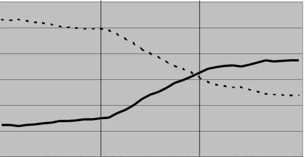
Figure I uses rolling regressions to show the dynamics of these changes. Panel A shows
how the dailybetas change overevent time. The solid lineshows the mean dailyS&P beta
andthe dashedlineshowsthe meandailynon-S&P beta. ThesecoeÆcientsarere-estimated
eachmonthusingtheprior12monthsofdailydata. Therefore coeÆcientsplottedtotheleft
oftheleftverticallineuseonlypre-eventreturns. CoeÆcientsplottedtotherightoftheright
verticallineuseonlypost-eventreturns. CoeÆcientsinbetweenusebothpre-andpost-event
data. In terms of these gures, the beta changes reported in Table 1 are the average beta
as of event month +12, which uses data frommonths [+1, +12] minusthe average beta as
returndata fora full24months afterinclusion. Tobeclear,the steady change inestimated
betas between the two vertical lines should not be interpreted as a steady change in true
betas. Rather, itarises frommixingdata fromthe pre- and post-event regimes.
Our results on changes in S&P and non-S&P betas are consistent with the ndings of
Vijh (1994),who studies whether the rise of S&P-linked products has aectedthe standard
measure of stock risk, namely beta with respect tothe overall marketreturn. He nds that
over the 1975-1989 period, a stock's daily beta with the market goes up by a statistically
signicant 0.08, on average, after inclusion. Since a large fraction of overall market value
comesfromS&Pstocks, thists withtheincrease inS&P beta wedetectoverasimilartime
period. Given our result that non-S&P beta falls signicantly, it also makes sense that the
rise in overall marketbeta should beconsiderably smallerthan the rise inS&P beta.
16
3.4 Evaluating Alternative Explanations
We now consider two alternative explanations for the results in Table 1 and Figure I. One
possibility is that stocks in the S&P 500 index dier from other stocks in terms of some
characteristic, and that the stocks Standard and Poor's chooses to include are stocks that
are increasingly demonstrating that characteristic. If the characteristic is also associated
with a cash-owfactor, this may explain our results.
The mostobvioussuchcharacteristicissize. Stocksinthe S&Phaveconsiderablyhigher
market capitalizations than stocks outside the index, and the stocks Standard and Poor's
includes into the index have often been growing in size prior to inclusion. Moreover, size
is associated with a cash-ow factor: there is a common component to news about the
earnings of large-cap stocks. Our nding that S&P betas increase around inclusion may
simply reect the fact that included stocks are growing in size around inclusion and are
therefore increasingly loading on the large stock cash-ow factor. More generally, this is a
story in which inclusion into the S&P coincides with a change in the cash-ow covariance
matrix, even if it doesnot cause it.
Another potential explanation is based onindustry eects. Suppose that some industry
becomes increasinglydominant in the economy. This increases the fraction of the value of
the S&P made up by stocks in this industry. Moreover, in an eort to keep their index
representative, Standard and Poor's may start drawing an increasing numberof new
inclu-sions fromthisindustry. Since S&Pbetaiscomputed usingthe value-weighted S&Preturn,
16
Under the CAPM, anincrease in overall market beta after inclusion predicts that stocks should drop
in pricewhentheyareaddedto theindex. Thefact that such stocksactuallydisplaylargepriceincreases
at precisely the time that other technology stocks in the index are growing in value { as
indeed it was, having been added in December 1999 { it may covary more with the S&P
afterinclusion than before.
Toaddressboththesecompetingexplanations,weperformamatchingexercise. Foreach
event stock included into the S&P during our sample period, we search for a \matching"
stock, drawn from the same industry as the event stock and in the same size decile as the
event stock, both at the time of inclusionand 12months before inclusion, but which is not
included intothe index. Inotherwords,sincethe matchingstockmatchestheeventstockon
industryandonrecentgrowthinmarketcapitalization,itisasgoodacandidateforinclusion
as the event stock itself,but simplyhappens not to be included. Ifthe matching stocks do
not demonstrate the same increase (decrease) in S&P (non-S&P) betas as the event stocks,
it strengthens the case that the results in Table 1 and Figure I are due to trading-based
comovement, rather than to the alternative explanations.
17
In the case of deleted stocks,
the matching stock is a stock inthe S&P which matches the deleted stock onindustry, and
recent change in marketcapitalization,but which isnot removed from the index.
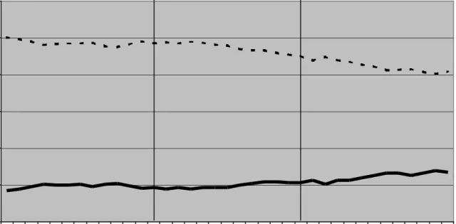
Table 2andFigureIIcontaintheresultsof thematchingexercise. FigureII,constructed
ina parallelfashion to FigureI, presents the evolution ofS&P and non-S&P betas in event
time for matching stocks. Table 2 reports the change in betas and R
2
in univariate and
bivariate regressions for event stocks relative tothe analogous changesfor matching stocks.
FigureIIsuggeststhatatdailyandweeklyfrequencies,thealternativestoriescanexplain
onlyasmallfractionof our results: thematchingstocksexhibitmuchsmallershiftsinbetas
than do the event stocks. However, it also suggests that at the monthly frequency, the
characteristic-andindustry-basedexplanationsdo havesomebite: even formatchingstocks,
S&P betas increase around inclusionand non-S&P betas decrease.
Table 2 conrms these impressions. At the daily and weekly frequency, the changes in
betaandR
2
inunivariateregressionsandinS&Pandnon-S&Pbetasinbivariateregressions,
remainstronglysignicantacrossinclusionevents,even aftersubtractingothe
correspond-ing changes for matching stocks. At the monthly level, however, a substantial part of the
strongbivariateregressionresultsinTable1are explainedbythematchingstocks.
Nonethe-less, in the second subsample, the increase in S&P beta for event stocks is stillsignicantly
17
Atthemonthlyfrequency,inordertomatchthewindowbetasarecomputedover,welookformatching
stocksthatmatchtheeventstockonsizebothatinclusionand36monthsbeforeinclusion.Atallfrequencies,
we initially tryto match by SIC4industry code. Ifno match can be found, weallow thematching stock
to bein thesameSIC3 industryclass, thentobewithin onesize decileat inclusion,thentobewithin one
size decile12 months before inclusion,then to be in thesame SIC2 industryclass, then to bewithin two
size deciles at inclusion, then to be within two size deciles 12 months before inclusion, and nally to be
withinthreesizedeciles12monthsbeforeinclusion. Eventsforwhichnosuchmatchescanbefoundarenot
greater thanthat formatching stocks.
Overall,itappears thattrading-basedcomovementoperatesstronglyatdailyandweekly
frequencies; atthe monthly frequency, itseects are stillpresent, but are less pronounced.
3.5 Calendar Time Tests
The methodology we use totest Propositions 1and 2 inSections 3.2and 3.3 is oftencalled
an\eventtime" approach. Analternativemethodology isa\calendartime" approach. This
technique is often used to address a common statistical problem in event studies, namely
correlationof returns acrossevents. As described inSection3.2., weuse simulationstodeal
with this issue. Performing calendar time tests oers a second way of checking that our
results are robust tothese statisticalconsiderations.
The calendar time approach requires the construction of two portfolios: a \pre-event"
portfoliowhose return attime t, R
pre;t
,is the equal-weighted averagereturn attime t of all
stocks that will be addedto the index withinsome windowaftertime t; and a\post-event"
portfolio whose return at time t, R
post;t
, is the equal-weighted average return at time t of
all stocks that have been added to the index within some window preceding time t. In our
analyses of daily and weekly data, we take the windowto be a year, and extend itto three
years for monthlydata.
The calendar time test of Proposition1 then calls for runningtwo regressions:
R pre;t = pre + pre R SP500;t +v pre;t (30) and R post;t = post + post R SP500;t +v post;t (31)
and checking whether
post
>
pre
and whether the R
2
in the second regression is greater
than inthe rst.
Similarly, the calendar time test of Proposition 2 calls for running the following two
regressions, R pre;t = pre + pre;SP500 R SP500;t + pre;nonSP500 R non SP500;t +v pre;t (32) and R post;t = post + post;SP500 R SP500;t + post;nonSP500 R nonSP500;t +v post;t (33) 18
InTable1,weconductedsimulationstocorrectthestandarderrorsforpossiblecorrelationindisturbance
termsacrossregressions.Thisproblemaectsmatchingstockregressionsjustasmuchasitdoeseventstock
regressions,butitdoesnotaectdierencesinslopesacrossthetwosetsofregressions.TheTable2standard
post;SP500 pre;SP500 post;nonSP500 pre;nonSP500
Table 3 reports the changes in slope coeÆcients and R
2
s. In general, the results are as
supportive of trading-based comovement as the event time tests. In the univariate
regres-sions, signicant increases in beta and R
2
occur at the daily and weekly frequencies, and
for R
2
;even at the monthlyfrequency. In the bivariate regressions, the results for inclusion
events are strongly signicantatallthree datafrequencies, althoughtheresults for deletion
events are weaker than before: there is nostatisticallysignicant eect at any frequency.
3.6 Comovement Across Categories
Proposition 3predicts that the correlationof the returns of two groups of securities willbe
lower than the correlation of their fundamentals if these groups form natural categories or
habitats. Thispropositionistestableinthe timeseries underthe conditionthat thegroups'
importanceas categories orhabitats has grown over time.
The S&P 500 satises this lastcondition: its use invariousinvestment styleshas grown
dramaticallyin the lastfew decades. Consistent with this trend, Wurgler and Zhuravskaya
(2001) nd that the size of the inclusion price jump has grown with the volume of funds
devotedtoS&Pindexing,andourearlierresultsshowincreasingcomovementeects inmore
recent years.
Table 4 reports the trends in comovement between the S&P and other stocks over the
past thirty years. The leftcolumnshowsthat the relativesize ofthe S&P andwholemarket
has remained constant. The declining correlations in the right columns show that at all
three data frequencies, the returns on the S&P 500 have grown increasinglydivorced from
the returns onthe rest of the market. The correlation inreturns remainshigh today, but it
isnotashighasitwaspriortotheadventoftheS&P500 asacategory. Anotherinteresting
patternisthatthe declineinthedailycorrelationseemstohavehaltedinrecentyears,while
the weekly and monthly correlationscontinue todecline.
In Table 5we determine whether the decreasing correlationbetween S&P and non-S&P
stocks is statistically signicant, or whether the correlation between two random groups
wouldonaveragedisplayasimilardecline. Weconstructvalue-weightedreturnsonarandom
group of 500 stocks and compute their correlation with the value-weighted returns on the
rest of the market overconsecutive veyear periods. Byrepeating this procedure for many
random groups of 500 stocks, we can construct sampling distributions for the change in
correlation over various intervals. We can then determine whether the decline in the S&P
correlation isunusually large.
groups of stocks have declined. Panel A shows that, fromthe early1970s to the late 1990s,
the daily return correlation between random groups has fallen by a median of -0.043. For
comparison, the secondcolumn fromthe rightreports the experience of the S&P 500. Over
this same period, Table 4 indicates that the dailyreturn correlation between the S&P and
the rest of the market has fallen by -0.118. The last column indicates that this is a much
greater declinethan expected by chance. A similar conclusion emerges for weekly data. At
the monthlylevel,the declinein correlationbetween S&P and non-S&P stocks isbelow the
average decline forrandomly-chosen stocks, but is not statistically unusual.
Our simulation controls for the possibility that the decline in the S&P and non-S&P
returncorrelationisduetoageneraldeclineinthecorrelationofstockfundamentals. Indeed,
the results of Campbell, Lettau, Malkiel, and Xu (2001) suggest that such a decline in
fundamentalcorrelationhasoccured, makingitimportanttocontrolfor. Oursimulationdoes
not, however, rule out the possibility that our results are due to an especially large decline
in the correlation of S&P 500 stocks' fundamentals with remaining stocks' fundamentals,
as compared to the decline in the correlation of a random 500 stocks' fundamentals with
remaining stocks' fundamentals. However, we see noobvious reason why this would be the
case,sincetheS&P500index hasalwaysbeenconstructedtoberepresentativeoftheoverall
economy. 19
4 Conclusion
In this paper, we present and examine empiricallythree models of comovement. The
tradi-tional model attributes comovement to correlation in news about fundamental value. The
twoalternativemodelsweconsiderexplaincomovementbycorrelatedinvestordemandshifts
for securities in agiven category,or by demand shifts by specic investor clienteles.
To assess these theories, we consider the well-studied phenomenon of stock inclusions
into, and deletions from,the S&P 500 index. While previous studies have noted signicant
immediate price eects associatedwith inclusionsand deletions, we focus onchangesin the
patterns of comovement of newly included (or deleted) stocks with stocks already in the
index. We nd that stocks included into the index begin tocomovemore with other stocks
inthe index,andlesswithstocks outoftheindex. The converseholdsfordeletions. Because
inclusionintothe S&P500 indexconveys nonews aboutfundamentals, thisevidenceishard
19
PanelAofTable4alsoshowsthattheabrupthaltinthedeclineofthedailyS&Pcorrelationafter1990
isnotmirroredbytherandom-500correlation,whiletheweeklyandmonthlyS&Pcorrelationscontinueto
declinerelativetothetypicalrandom-500group. Oneexplanationisthatarbitragehascheckedthedecline
inthedailycorrelation,buthasyetto stopthedeclinein theweeklyandmonthlycorrelations. DeLonget
shifts indemand.
This evidenceaddstothegrowingrange ofphenomenaidentiedbynancialeconomists
that reveal the importanceof asset classication,and of demand shifts amongasset classes,
for valuation. From this perspective, a security's price may depend not only on its
fun-damentals, but also on which asset categories it belongs to, and on which investors trade
Proof of Propositions 1, 2, and 3: Suppose that asset n+1 is reclassied from Y into X,
and that at the same moment,asset 1is reclassied from X into Y. Beforereclassication,
P X ;t+1 = " X ;t+1 + u X ;t+1 1 + u Y;t+1 2 (34) P Y;t+1 = " Y;t+1 + u X ;t+1 2 + u Y;t+1 1 P n+1;t+1 = " n+1;t+1 + u X ;t+1 2 + u Y;t+1 1 ; where " k;t = 1 n X l k " l ;t , k =X;Y. This implies, asn !1; cov (P n+1;t+1 ;P X ;t+1 ) = 2 M + 2 2 u 1 2 + 2 u u ( 1 2 1 + 1 2 2 ) (35) cov (P n+1;t+1 ;P Y;t+1 ) = 2 M + 2 S + 2 u ( 1 2 1 + 1 2 2 )+ 2 2 u u 1 2 var(P X ;t+1 ) = var(P Y;t+1 )= 2 M + 2 S + 2 u ( 1 2 1 + 1 2 2 )+ 2 2 u u 1 2 cov (P X ;t+1 ;P Y;t+1 ) = 2 M + 2 2 u 1 2 + 2 u u ( 1 2 1 + 1 2 2 ): After reclassication, P X ;t+1 and P Y;t+1
are stillgiven by (34), but now
P n+1;t+1 =" n+1;t+1 + u X ;t+1 1 + u Y;t+1 2 : (36) This implies, asn !1; cov (P n+1;t+1 ;P X ;t+1 ) = 2 M + 2 u ( 1 2 1 + 1 2 2 )+ 2 2 u u 1 2 ; (37) cov (P n+1;t+1 ;P Y;t+1 ) = 2 M + 2 S + 2 2 u 1 2 + 2 u u ( 1 2 1 + 1 2 2 ); while var(P X ;t ), var(P Y;t ), and cov(P X ;t+1 ;P Y;t+1
)remain the same as before.
Since the OLS estimateof
n+1 in the regression P n+1;t+1 = n+1 + n+1 P X ;t+1 +v n+1;t+1 (38) is given by n+1 = cov (P n+1;t+1 ;P X ;t+1 ) var(P X ;t+1 ) ; (39)
1 2 1 + 1 2 2 2 1 2 =( 1 1 1 2 ) 2 0; conrmthat n+1
increasesafterreclassicationasclaimedinProposition1. Moreover, since
var(P n+1;t
) and var(P
X ;t
) are unchanged after reclassication, the increase in
n+1 also
implies anincrease in R
2
of regression (38) afterinclusion.
The OLS estimates of
n+1;X and n+1;Y inthe regression P n+1;t+1 = n+1 + n+1;X P X ;t+1 + n+1;Y P Y;t+1 +v n+1;t+1 (40) are given by n+1;X n+1;Y ! = 1 V X V Y C 2 XY V Y C XY C XY V X ! C n+1;X C n+1;Y ! (41) where V k = var(P k;t+1 ); k =X;Y C XY = cov (P X ;t+1 ;P Y;t+1 ) C n+1;k = cov (P n+1;t+1 ;P k;t+1 ),k =X;Y. Before reclassication, C n+1;X = C XY and C n+1;Y = V Y
, while after reclassication,
C n+1;X =V X 2 S and C n+1;Y =C XY + 2 S
. It iseasy tocheck that thisimplies that
n+1;X
does indeedincrease afterreclassication, while
n+1;Y
falls. This proves Proposition 2.
Finally,given the expressions for var(P
X ;t+1 ),var(P Y;t+1 ),and cov(P X ;t+1 ;P Y;t+1 )
in equation(35), it isimmediate that
corr(P X ;t+1 ;P Y;t+1 )<corr(D X ;t+1 ;D Y;t+1 ):
Barberis, N., and A. Shleifer (2003), \Style Investing," forthcoming, Journal of Financial
Economics.
Bodurtha J., Kim, D., and C.M. Lee (1995), \Closed-end Country Funds and U.S. Market
Sentiment," Review of FinancialStudies 8, 879-918.
Campbell,J.Y.,Lettau,M.,Malkiel,B.,andY.Xu(2001),\HaveIndividualStocksBecome
More Volatile? An Empirical Exploration of Idiosyncratic Risk," Journal of Finance 56,
1-43.
De Long, J.B., Shleifer A., Summers L., and R. Waldmann (1990), \Noise Trader Risk in
Financial Markets," Journal of PoliticalEconomy 98,703-38.
Fama, E., and K. French (1993), \Common Risk Factors in the Returns on Stocks and
Bonds," Journal of Financial Economics 33, 3-56.
Fama, E., and K. French (1995), \Size and Book-to-Market Factors in Earnings and
Re-turns," Journal of Finance 50,131-155.
French, K., and R. Roll (1986), \Stock Return Variances: The Arrival of Information and
the Reaction of Traders," Journal of FinancialEconomics 17, 5-26.
Froot,K., andE.Dabora(1999),\Howare StockPricesaectedbytheLocationofTrade?,"
Journal of Financial Economics 53,189-216.
Goetzmann, W., and M. Massa (2001), \Index funds and stock market growth," Working
Paper, YaleUniversity.
Gompers, P., and A.Metrick (2001), \InstitutionalInvestors and Equity Prices," Quarterly
Journal of Economics 116, 229-259.
Greenwood, R. (2001), \Large Events and Limited Arbitrage: Evidence from a Japanese
Stock Index Redenition," Working Paper, Harvard University.
Greenwood, R., and N. Sosner (2002), \Where Do Betas Come From?," Working Paper,
Harvard University.
Hardouvelis,G.,LaPortaR.,and T. Wizman (1994),\What Movesthe Discounton
Coun-try Equity Funds?," in Jerey Frankel (ed.), The Internationalization of Equity Markets,
the S&P 500: New Evidence for the Existence of Price Pressure," Journal of Finance 41,
851-860.
Kaul, A., Mehrotra V., and R.Morck (2000), \Demand Curves for Stocks Do Slope Down:
New Evidence from anIndex Weights Adjustment," Journal of Finance 55,893-912.
Lamont,O.,and R.Thaler(2000), \Canthe MarketAddand Subtract? MispricinginTech
Stock Carveouts," Working Paper, University of Chicago.
Lee, C., Shleifer A., and R. Thaler (1991), \Investor Sentiment and the Closed-end Fund
puzzle," Journal of Finance 46,75-110.
Lynch, A. and R. Mendenhall (1997), \New evidence on stock price eects associated with
changes in the S&P 500 Index," Journal of Business 70,351-83.
Merton, R.(1987), \ASimple Model of CapitalMarket Equilibriumwith Incomplete
Infor-mation,"Journal of Finance 42, 483-510.
Mitchell, M., Pulvino, T., and E. Staord (2002), \Limited Arbitrage in Equity Markets,"
forthcoming, Journal of Finance.
Pindyck, R., and J. Rotemberg (1990), \The Excess Comovement of Commodity Prices,"
Economic Journal 100, 1173-1189.
Pindyck,R.andJ.Rotemberg(1993),\TheComovementofStockPrices,"QuarterlyJournal
of Economics 108, 1073-1104.
Shiller,R.(1989), \Comovementsin StockPrices and ComovementsinDividends," Journal
of Finance 46,719-729.
Shleifer A. (1986), \Do Demand Curves for Stocks Slope Down?," Journal of Finance 41,
579-590.
ShleiferA., andR. Vishny(1997),\The Limitsof Arbitrage,"Journal of Finance 52, 35-55.
Vijh,A.(1994),\S&P500TradingStrategies andStockBetas,"Review of FinancialStudies
7,215-251.
Wurgler, J., and K. Zhuravskaya (2001), \Does Arbitrage Flatten Demand Curves for