Exemplar and Prototype Models Revisited: Response Strategies, Selective Attention, and Stimulus Generalization

Exemplar and Prototype Models Revisited: Response Strategies,

Selective Attention, and Stimulus Generalization

Robert M. Nosofsky and Safa R. Zaki

J. D. Smith and colleagues (J. P. Minda & J. D. Smith, 2001; J. D. Smith & J. P. Minda, 1998, 2000; J. D. Smith, M. J. Murray, & J. P. Minda, 1997) presented evidence that they claimed challenged the predictions of exemplar models and that supported prototype models. In the authors’ view, this evidence confounded the issue of the nature of the category representation with the type of response rule (probabilistic vs. deterministic) that was used. Also, their designs did not test whether the prototype models correctly predicted generalization performance. The present work demonstrates that an exemplar model that includes a response-scaling mechanism provides a natural account of all of Smith et al.’s experimental results. Furthermore, the exemplar model predicts classification performance better than the prototype models when novel transfer stimuli are included in the experimental designs.

A classic issue in cognitive psychology concerns the manner in which people represent categories in memory. According to pro-totype models (Homa, 1984; Posner & Keele, 1968; Reed, 1972), people represent categories by forming a summary representation that is a central tendency of all of the experienced members of a category. Classification decisions are based on the similarity of an item to the alternative prototypes. By contrast, according to exem-plar models (Hintzman, 1986; Medin & Schaffer, 1978; Nosofsky, 1986), people represent categories by storing the individual mem-bers or exemplars of a category as separate traces and classify items based on their similarity to these stored exemplars.

There is a good deal of converging evidence that prototype models are insufficient as models of categorization, especially in situations in which learners have been repeatedly exposed to the individual exemplars of each category. Memories for the individ-ual exemplars appear to play at least some role in such situations (Homa, Sterling, & Trepel, 1981; Posner & Keele, 1968; Nosof-sky, 1992; Smith & Minda, 2000).

Conversely, however, in a recent series of articles, Smith and colleagues (Minda & Smith, 2001; Smith & Minda, 1998, 2000; Smith, Murray, & Minda, 1997) have presented evidence that they claim severely challenges exemplar models of categorization. These researchers argue that the formation of prototypes serves as a first organizing principle in the representation of categories. They hypothesize that, especially at early stages of learning, peo-ple’s category representations are prototype based. With continued learning on a restricted set of exemplars, people may eventually form memories for those exemplars and use those memories to

classify the old training instances. However, generalization to new items is still assumed to be governed by similarity to the prototype. In this article we question the evidence that Smith et al. (1997; Smith & Minda, 1998) have advanced in favor of the prototype hypothesis and against the exemplar view. Specifically, we argue that a current exemplar-based generalization model of categoriza-tion provides a natural account of all of their results. Furthermore, we present evidence that their alternative “mixed model” of cate-gorization, which involves a combination of prototype-based rep-resentation together with all-or-none memories for specific exem-plars, fails to predict correctly people’s classification performance. We organize our article by first presenting the main competing models of classification that serve as representatives of the proto-type and exemplar views. Next, we review the key experimental paradigm and sources of evidence that Smith et al. have used to challenge the exemplar-generalization model and to support the prototype model. We then explain why we believe that Smith and colleagues’ paradigm and results fail to discriminate between these alternative modeling approaches and suggest that their data pro-vide little epro-vidence for the operation of a broad-based prototype-abstraction process. Finally, we report a new series of experiments to corroborate our interpretations and to develop contrasts between the predictions from the exemplar-generalization and mixed-prototype models.

Review of the Models

In this section we review the various models that serve as rep-resentatives of the exemplar, prototype, and mixed-representation views. In the experimental paradigms under consideration, all of the models are compared in situations in which the stimuli are composed of binary-valued, separable dimensions and in which subjects are classifying the stimuli into one of two categories. For simplicity, we describe the models as they are applied in such a paradigm, although extensions of the models to more general paradigms are straightforward (e.g., Nosofsky, 1986, 1987; Shin & Nosofsky, 1992).

Robert M. Nosofsky and Safa R. Zaki, Department of Psychology, Indiana University Bloomington.

This work was supported by National Institute of Mental Health Grant R01 MH48494. We thank Michael Erickson and two anonymous reviewers for their helpful criticisms of an earlier version of this article.

Correspondence concerning this article should be addressed to Robert M. Nosofsky, Department of Psychology, Indiana University, Blooming-ton, Indiana 47405. E-mail: [email protected]

Exemplar-Generalization Model

The representative of the class of exemplar-generalization mod-els is the context model of classification proposed by Medin and Schaffer (1978), generalized by Nosofsky (1984, 1986), and fur-ther extended by Ashby and Maddox (1993). According to the model, the probability that item i is classified into Category A is given by

P共A兩i兲⫽ 共

冘

␥

共

冘

冘

, (1)

where兺siaand兺sibdenote the summed similarities of item i to

the exemplars of Categories A and B, respectively, and ␥ is a response-scaling parameter (Ashby & Maddox, 1993; McKinley & Nosofsky, 1995). The ␥parameter, introduced into the context-model response rule by Ashby and Maddox (1993), governs the extent to which responding is probabilistic versus deterministic. When␥⫽1, observers respond probabilistically by “matching” to the relative summed similarities of each category, whereas when␥ grows greater than 1, observers respond more deterministically with the category that yields the larger summed similarity.

Issues pertaining to the␥response-scaling parameter are critical to evaluating the comparisons between exemplar and prototype models conducted by Smith et al. (1997; Minda & Smith, 2001; Smith & Minda, 1998). In all of the model comparisons that they conducted, these researchers set␥ ⫽ 1 in the exemplar model. However, previous research has demonstrated that this constrained version of the exemplar model is inadequate because it fails to account for the deterministic patterns of responding that are often evidenced at the individual subject level (e.g., Ashby & Gott, 1988; Ashby & Maddox, 1993; Maddox & Ashby, 1993; McKin-ley & Nosofsky, 1995; Nosofsky, 1991a). Much of our discussion in the present article involves reviewing the importance of the␥ response-scaling parameter and demonstrating that analogous forms of response scaling are just as important to prototype-based accounts of classification performance as to exemplar-based accounts.

According to the context model, in situations involving binary-valued, separable dimensions, the distance between exemplars i and j is given by

dij⫽

冘

m⫽1

M

wm䡠兩xim⫺xjm兩, (2)

where xim and xjm denote the values of exemplars i and j on

dimension m, respectively, wmis the “attention weight” given to

dimension m, and M denotes the number of dimensions along which the stimuli vary. The attention-weight parameters are con-strained to vary between 0 and 1 (0ⱕwmⱕ1) and to sum to 1.

Note that because the dimensions are binary-valued, each compo-nent兩xim⫺ xjm兩is equal either to 0 (if exemplars i and j match

on dimension m) or to 1 (if the exemplars mismatch on this dimension).

The selective attention process formalized in Equation 2 is an essential aspect of the exemplar-based context model. As dis-cussed by Medin and Schaffer (1978) in their original formulation of the model, the selective attention process may capture the types of “hypothesis testing” behavior presumed to underlie

classifica-tion performance, especially at early stages of learning. In addi-tion, there is evidence that with extended training, observers often learn to distribute attention across dimensions in a manner that tends to optimize performance (e.g., Nosofsky, 1984, 1986, 1991a).

The similarity between exemplars i and j is an exponential decay function of their distance (Shepard, 1987),

sij⫽exp(⫺c䡠dij), (3)

where c is an overall sensitivity parameter that determines the rate at which similarity declines with distance. As explained in numer-ous previnumer-ous articles, the combination of the “city-block” distance metric formalized in Equation 2 and the exponential similarity function formalized in Equation 3 yields an interdimensional mul-tiplicative rule for computing similarity (see Medin & Schaffer, 1978; and Nosofsky, 1984, for more extensive discussion). As a result, the context model is often referred to as a multiplicative-similarity exemplar model.

The similarities computed from Equations 2 and 3 are substi-tuted into Equation 1 to yield the classification probabilities that are predicted by the model. The free parameters in the model are the response-scaling parameter␥, the sensitivity parameter c, and

M⫺1 freely varying attention weights (wm).

Additive-Prototype Model

In the various prototype models under consideration, a prototype vector is defined for each of Categories A and B. The prototype for Category A is composed of the dimension values that occur most frequently among the members of Category A, and likewise for the prototype of Category B. According to the additive-prototype model advanced by Smith et al. (1997; Smith & Minda, 1998), when item i is presented, the evidence in favor of a Category A response is given by

Ei,A⫽

冘

where wmis the attention weight given to Dimension m (just as in

the context model’s Equation 2); and␦mis an indicator variable set

equal to 1 if item i matches the prototype of Category A on dimension m, and set equal to zero if it mismatches the prototype of Category A on this dimension. The probability that an observer classifies item i into Category A is given by

P共A兩i兲⫽g

2⫹共1⫺g兲䡠Ei,A, (5)

where g (0 ⱕ g ⱕ 1) is a guessing parameter. That is, with probability g the observer guesses randomly between the two categories, and with probability (1 ⫺ g) the observer uses the

prototype-based evidence to make a response. The guessing pa-rameter is critical to the additive-prototype model if it is to make plausible predictions of classification performance. If g⫽0, then the item that is the prototype of each category is predicted to be classified with probability 1 into its correct category. The guessing parameter allows the additive-prototype model to account for the less-than-perfect performance that is sometimes observed for the prototype patterns.

Note that the additive-prototype model advanced by Smith et al. (1997; Smith & Minda, 1998) does not include a response-scaling

parameter. In the section The Prototype-Plus-Exception Structure, we explain why this highly simplified model is often sufficient to account for performance at very early stages of classification learning. We go on to demonstrate in our subsequent experiments, however, that this highly simplified model is quite limited in generality. Even if the category representation is prototype based, we demonstrate that the additive-prototype model needs to be augmented with a response-scaling parameter, analogous to the one found in the context model.

Multiplicative-Prototype Model

Besides assuming a different category representation, the con-text model and the additive-prototype model differ in the rules that are used to compute “similarity,” that is, the context model uses a multiplicative rule whereas the additive-prototype model uses an additive rule. To improve the comparability between the models, Estes (1986) and Nosofsky (1987, 1992) introduced a multiplica-tive version of the prototype model that uses the same similarity functions as the context model. The distance between item i and Prototype A is given by

diA⫽

冘

where PAmdenotes the value of Prototype A on dimension m, and

the wmare the attention weights. The similarity between item i and

Prototype A is then given by

siA⫽exp共⫺c䡠diA), (7)

where c is the sensitivity parameter. Analogous equations are used to compute the similarity of item i to Prototype B. The probability with which item i is classified into Category A is given by

P共A兩i兲⫽g

2⫹共1⫺g兲䡠 siA

siA⫹siB

. (8)

A response-scaling parameter ␥ could be added to the multiplicative-similarity prototype model in a manner analogous to the context model (Equation 1). Critically, however, within the framework of the multiplicative-similarity prototype model, the␥ parameter cannot be estimated separately from the sensitivity parameter c. That is, without loss of generality, the␥parameter in the multiplicative-prototype model can be set equal to one and its influence absorbed by the sensitivity parameter c. To see why, let

P共A兩i兲⫽ siA

␥ siA␥⫹siB␥

. (9)

Note that siA␥⫽[exp(⫺c䡠diA)]␥⫽exp(⫺c䡠␥䡠diA)⫽exp(⫺c⬘䡠 diA), where c⬘ ⫽ c䡠␥. Thus, the role of the␥response-scaling

parameter is already implicit in the multiplicative-prototype model.1

We discuss this crucial issue in greater depth in the section The Response-Scaling Parameter␥.

Mixed Model

As discussed by Smith and Minda (1998, 2000), with extended training on a fixed set of exemplars, there is evidence that stored exemplars come to play an important role in influencing classifi-cation performance. However, these researchers hypothesized that the memories of these exemplars are “all-or-none” in the sense that

they are used only for purposes of classifying the training instances themselves. Generalizations to new items are assumed to be based solely on similarity comparisons to the prototypes. Smith and Minda (2000; pp. 9 –10, 13–18) argued strongly that this all-or-none exemplar memory assumption is simpler and psychologically more plausible than is the exemplar-similarity process formalized in the context model. Thus, according to Smith et al.’s (1997; Minda & Smith, 2001; Smith & Minda, 1998, 2000) proposed mixed model of classification, the probability that an old training instance from Category A is correctly classified into Category A is given by

P共A兩i兲⫽e⫹共1⫺e兲䡠g

2⫹共1⫺e兲䡠共1⫺g兲䡠proto共A兩i兲, (10) where e (0ⱕeⱕ1) is the probability that the observer has formed a memory trace for an individual exemplar, g is the guessing probability, and proto (A兩i) denotes the probability that item i is

classified into Category A by the prototype process. If item i is a new item that was not presented during training, then e⫽0 and classification is based solely on a combination of the guessing and prototype processes. In our research we considered two different versions of the mixture model, one that assumed an additive-prototype process and the other that assumed a multiplicative-prototype process.

The Response-Scaling Parameter

␥

In the original formulation of the exemplar-based context model, Medin and Schaffer (1978) assumed that classification responses were based on matching to the relative summed simi-larities of each category. That is, they assumed ␥ ⫽ 1 in the response rule formalized in Equation 1. There was never any strong theoretical justification for the use of this response rule, however.2

For example, Medin and Smith (1981) wrote, “The best defense of the response rule is that it is a fair approximation and that it seems to work” (p. 250). Indeed, when one uses the context model to fit classification data averaged across subjects, the model

1_{By contrast, because the exemplar model involves a summing of} similarities (see Equation 1), the␥response-scaling parameter is mathe-matically distinct from the sensitivity parameter in that model. We note, however, that even in the exemplar model, there are situations in which it is difficult to estimate separately the values of these two parameters.

2_{One possible source of justification is the relation between the} context-model response rule and the classic similarity-choice context-model (SCM) of stimulus identification (Luce, 1963; Shepard, 1957), which does not include the␥response-scaling parameter. According to the SCM, the probability that stimulus i is identified as stimulus j is given by P(j兩i) ⫽

冘

bk␩*ik , where bjis the bias for response j and␩*_ijis the similarity between stimuli

i and j. For the same reason as in the multiplicative-prototype model,

however, the␥response-scaling parameter is nonidentifiable within the framework of the SCM. Thus, the model P(j兩i) ⫽ bj␩ij

␥

冘

is formally identical to the standard version with␩*_ij⫽␩ij␥. If similarity in the SCM is assumed to be an exponential decreasing function of distance in psycho-logical space (Shepard, 1957), then the ␥ response-scaling parameter cannot be estimated separately from the sensitivity parameter c.

with␥⫽1 tends to fit quite well. However, numerous independent lines of evidence since then have indicated that when fitting individual subject data with the exemplar model, it is important to allow␥to take on values greater than 1 (e.g., Maddox & Ashby, 1993; McKinley & Nosofsky, 1995; Nosofsky & Palmeri, 1997; see also Nosofsky, 1991a, for a slightly different version of a deterministic exemplar model). As previously discussed in the Review of the Models section, the␥response-scaling parameter describes the extent to which observers use deterministic versus probabilistic response strategies, and values of ␥⬎ 1 allow the exemplar model to account for the levels of deterministic respond-ing that are often evidenced by individual subjects (Ashby & Gott, 1988; Lovett, 1998; Ross & Murphy, 1996).

A process interpretation for the emergence of the ␥parameter was provided by Nosofsky and Palmeri (1997) in the form of their exemplar-based random-walk (EBRW) model of classification. In that model,␥corresponds to the magnitude of the response criteria in a random-walk process in which exemplars are retrieved from memory; that is, it corresponds to the amount of exemplar-based evidence that needs to be obtained before an observer will initiate a response (see Nosofsky & Palmeri, 1997, p. 291).

Indeed, essentially all modern models of classification include a response-scaling parameter that is analogous to ␥, including the response-scaling constant␸in Kruschke’s (1992) attention learn-ing coverlearn-ing map (ALCOVE) model (see Kruschke, 1992, p. 24), the goal-value parameter G and response-noise parameter t in Anderson and Lebiere’s (1998) adaptive control of thought– revised (ACT–R) theory (see Lovett, 1998, pp. 256 –257, 276 – 277), and the criterial-noise parameter␴c

2

in Ashby and Maddox’s (1993) decision-bound theory (see Ashby & Maddox, 1993, pp. 377–378).

Smith et al. have strongly criticized the role of the response-scaling parameter␥in the context model. For example, Smith and Minda (1998) argued that␥functions to allow the exemplar model to mimic what is in truth a prototype-based process, suggesting that the response-scaling parameter “can be a prototype in exem-plar clothing” (p. 1431). Likewise, Minda and Smith (2001, p. 794) argued that including the␥parameter in the context model left the competing exemplar and prototype models unbalanced in their assumptions and parameters and endowed the exemplar model with too much flexibility. These arguments did not recognize, however, that the multiplicative-similarity prototype model itself already contains the formal flexibility that in essence accommo-dates a response scaling parameter (see our previous section, Review of the Models). Not including the ␥ parameter in the exemplar model creates a lack of balance in favor of the multiplicative-similarity prototype model, at least with respect to response-scaling processes.

Finally, although the additive-prototype model does not cur-rently include a response-scaling parameter, one of our initial goals for the present article is to demonstrate the limited generality of this proposed model, even if it is extended by the all-or-none exemplar-memory process proposed by Smith et al. (Minda & Smith, 2001; Smith & Minda, 1998, 2000). In our next section, we suggest that the additive-prototype model has fared well in Smith et al.’s experimental paradigm for a very special reason, and we argue that somewhat more challenging paradigms can quickly reveal the inadequacy of this model.

The Prototype-Plus-Exception Structure

The main experimental paradigm used by Smith et al. for demonstrating a purported qualitative advantage of the prototype models over the exemplar model is shown in Table 1. There are seven training exemplars in each of two categories, A and B. Each exemplar varies along six binary-valued dimensions, with logical value 1 on each dimension tending to indicate Category A and logical value 2 tending to indicate Category B. In this design, Stimulus 1 (111111) is the prototype of Category A, whereas Stimulus 8 (222222) is the prototype of Category B. Note also that each category contains an “exception” item. Stimulus 7 (222212) is the exception stimulus that belongs to Category A, whereas Stimulus 14 (111211) is the exception stimulus that belongs to Category B. All of the remaining exemplars in each category differ from their respective prototypes along just a single dimension. We refer to these items as the low distortions of the prototype.

Smith et al. (1997, Smith & Minda, 1998) tested designs in which subjects learned to classify these 14 training instances into each of the two categories. They then fitted the various competing models to the classification learning data of each of their individ-ual subjects. They found that at early stages of learning, the prototype models provided better fits to the classification data than did the exemplar model (with␥⫽1), at least for certain subsets of the subjects who were tested.

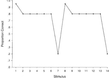
To characterize the limitations of the exemplar model, Smith et al. (1997) created composite plots showing the observed and predicted percentage of correct responses for each individual stim-ulus. (Although the models were fitted to the data of each indi-vidual subject, the composite plots were created by averaging across the observed and predicted data of the subjects.) An exam-ple of one such plot is provided in Figure 1, which shows the predictions from the exemplar model and the observed data from a subset of subjects who showed a “prototype-based” pattern of performance. The key aspect of the plot emphasized by Smith et al. (1997) is that the exemplar model underestimates the predicted percentage of correct responses for the prototype patterns (Stim-uli 1 and 8) and overestimates the predicted percentage of correct responses for the exception patterns (Stimuli 7 and 14). By con-trast, these systematic deviations were not present in the prototype-model fits to this subset of subjects.

Consider the following highly simplified process that might be taking place when observers learn to classify the stimuli in this paradigm. Numerous studies suggest that at early stages of learn-ing involvlearn-ing separable-dimension stimuli, observers may engage

Table 1

The Prototype-Plus-Exception Structure Tested by Smith et al. (1997; Smith & Minda, 1998) and in Experiments 2 and 3 of the Present Research

Category A Category B 1. 111111 8. 222222 2. 211111 9. 122222 3. 121111 10. 212222 4. 112111 11. 221222 5. 111121 12. 222122 6. 111112 13. 222221 7. 222212 14. 111211

in hypothesis-testing behavior in which they sample rules along individual dimensions (Levine, 1975; Medin & Schaffer, 1978; Nosofsky, Palmeri, & McKinley, 1994; Trabasso & Bower, 1968). Thus, suppose that an observer formed a rule along Dimension 1. Any stimulus with value 1 along Dimension 1 would be classified into Category A, whereas any stimulus with value 2 along Dimen-sion 1 would be classified into Category B. Each individual sub-ject, however, might form a rule along a different dimension. For simplicity, we assume that the rule dimension is chosen randomly for each subject. Finally, analogous to the guessing process for-malized in the prototype models, subjects might guess randomly between the categories on some proportion g of the trials. The composite predictions generated by this highly simplified model with g⫽.10 are displayed in Figure 2. Remarkably, this highly simplified “rule” model, in which each observer is making use of information along just a single dimension, yields the type of composite profile reported by Smith et al. (1997) in their studies. (A more precise quantitative fit could be achieved by estimating as free parameters the probabilities with which individual subjects adopted rules along the different dimensions.) Later in our article, we analyze the data from individual observers to provide evidence that a process not very different from this highly simplified rule-based process may indeed underlie classification behavior at the very early stages of learning.

This pattern of classification responding, however, does not constitute evidence that people are using prototype-based strate-gies rather than exemplar-based stratestrate-gies, as Smith et al. claim. The additive-prototype and multiplicative-prototype models would fit such individual performances simply by placing all of their attention weight on the single rule dimension. Likewise, the ex-emplar model would fit such performances equally well by placing all of its attention weight on this single dimension.

(Single-dimension rules of this form are a very special case of the types of behavior that the selective-attention exemplar model was designed to explain—see, e.g., Medin & Schaffer, 1978; Nosofsky, 1984, 1986, 1991b.) However, the value of ␥in the exemplar model would need to be set at a sufficiently high value to account for the deterministic pattern of responding assumed in the rule-based process.

As discussed previously, in all of their previous quantitative tests of the exemplar model, Smith et al. (1997; Minda & Smith, 2001; Smith & Minda, 1998) held␥fixed at 1. Suppose that an observer attended selectively to Dimension 1 and gave zero atten-tion to the remaining dimensions. Note from Table 1 that five of the seven exemplars from Category A have logical value 1 on Dimension 1, whereas two of the seven exemplars from Category B have logical value 1 on this dimension. Applying the exemplar model with␥⫽1, one can directly show that the model predicts, for example, that the prototype of Category A will be classified correctly with maximum probability 5/(5⫹2)⫽.71, which is far less than the observed average proportion correct of over .90 reported in the composite plot of Figure 1. This underprediction, we believe, lies at the heart of essentially all of Smith et al.’s demonstrations of the limitations of the exemplar model.

Our view, however, is that constraining the exemplar model to match to the relative summed similarities, as is the case in the ␥⫽1 model, is arbitrary. From a psychological point of view, an observer at early stages of learning may remember that five ex-emplars from Category A had value 1 on Dimension 1 and that two exemplars from Category B had value 1 on Dimension 1. When tested with an object that has value 1 on Dimension 1, a subject’s reasonable response strategy would simply be to classify it into Category A, as would be predicted by a deterministic version of the exemplar model with␥set at a sufficiently high level.

The plan in the remainder of our article is as follows. We start by reporting something of a “demonstration” experiment to show clearly that the additive-prototype model is inadequate as a model of classification performance, even if augmented with an

all-or-Figure 2. Composite predictions generated by a highly simplified single-dimension rule model for the prototype-plus-exception structure tested by Smith et al. (1997; Smith & Minda, 1998). Compare the form of the plot to the observed data in Figure 1.

Figure 1. The solid line shows the average observed percentage of correct category decisions displayed by the “prototype subjects” for each of the 14 stimuli in Smith et al.’s (1997) Experiment 1 (nonlinearly separable, easy condition). The dotted line shows the average percentage of correct category decisions for each stimulus predicted by the exemplar-based context model with␥⫽1. From “Straight Talk About Linear Separabil-ity,” by J. D. Smith, M. J. Murray, and J. P. Minda, 1997, Journal of

Experimental Psychology: Learning, Memory, and Cognition, 23, p. 669.

Copyright 1997 by the American Psychological Association. Adapted with permission of the authors.

none exemplar memory process. Just as is the case with the exemplar model and the multiplicative-prototype model, the additive-prototype model too needs to be endowed with a response-scaling mechanism.

Next, we conduct a replication and extension of the key exper-imental paradigm used by Smith et al. that purportedly found evidence for a prototype-abstraction process. Detailed analyses of the individual subject data obtained at early stages of learning suggest that rather than having adopted a broad-based prototype, as might be conveyed by inspecting the composite plot in Figure 1, individual subjects are indeed attending selectively to a small subset of the stimulus dimensions, very much in the spirit of the simple rule-based process used to generate our Figure 2. The predictions from exemplar and prototype models can simply not be distinguished in such a situation.

In a final experiment, we follow Smith and Minda (1998) by having subjects learn the prototype-plus-exception structure in a more extended training session. To learn the category structure, subjects must spread their attention to other relevant dimensions of the objects. Critically, however, whereas Smith and Minda (1998) tested observers on only the old training instances, in our experi-ment we extend the paradigm by also testing how observers generalize to new transfer stimuli. This extension allows the pre-dictions from the exemplar and prototype models to be sharply distinguished. Model-based analyses of the individual subject data from such a paradigm reveal that the standard exemplar-generalization model provides a dramatically better account of the observed classification performance than do the alternative proto-type models, even ones that are augmented with an all-or-none exemplar-memory process.

Experiment 1

The purpose of Experiment 1 was to provide a simple demon-stration of the limitations of the additive-prototype model, even if this model is augmented with the all-or-none exemplar-memory process.

The key manipulation in our experiment was to train individual observers on only the actual prototypes of each category. The stimuli were composed of six binary-valued dimensions. To lessen the possibility that observers would attend selectively to only a single dimension (or to just a few dimensions), we provided observers with explicit instructions that each dimension of the objects was equally important. Finally, in a transfer phase, we tested subjects not only with the prototypes on which they were trained but also with various new transfer stimuli that were dis-tortions of the prototypes. Low disdis-tortions differed by one dimen-sion value from their prototype and medium distortions differed by two dimension values. To ensure highly motivated subjects, we provided payoffs for good performance. The subjects were not provided with feedback on the various transfer patterns but were told that there were right and wrong answers and that they would be paid on the basis of their performance.

Because only the prototypes were presented as training exem-plars, the context model and the multiplicative-prototype model are formally identical in this experimental paradigm. The purpose of the paradigm was to sharply distinguish the multiplicative-similarity models from the additive-prototype model. The intuition here is straightforward. Presumably, an observer wishing to

max-imize payoffs would classify an object into Category A if it were more similar to the Category A prototype than to the Category B prototype, and vice versa for Category B objects. Thus, observers should respond in near deterministic fashion, with correct choice probabilities close to 1.0 for all patterns (as long as the observers distribute their attention across all of the dimensions of the ob-jects). The multiplicative-similarity models account for such per-formance in a straightforward fashion simply by setting the response-scaling (or sensitivity) parameter at a sufficiently high level. By contrast, without a response-scaling process, the additive-prototype model is constrained to make much different predictions. Assuming, for example, that observers distribute at-tention equally among the six dimensions (i.e., so that each wm

attention-weight parameter in Equation 4 has a value of .167), then low distortions are predicted to be correctly classified with max-imum probability .833 and medium distortions are predicted to be correctly classified with maximum probability .667. Furthermore, making allowance for the idea that observers supplement the prototype process by forming all-or-none memories for the train-ing patterns does nothtrain-ing to save the additive-prototype model because the only training patterns are the prototypes themselves.

Method

Subjects. Eight Indiana University graduate students were paid $7 for participating in the experiment. In addition, subjects were given a bonus of $3 if they achieved at least 95% correct in the task. We tested graduate students and used payoffs because achieving a clear demonstration of the inadequacies of the additive-prototype model requires that subjects per-form at high levels. None of the subjects was aware of the issues under investigation in this study.

Stimuli. The stimuli were the six-letter nonsense words used by Smith et al. (1997; Smith & Minda, 1998) in some of their experiments. Each letter in the nonsense strings is presumed to constitute a feature. There were four prototype pairs (HAFUDO–NIVETY; GAFUZI–WYSERO; BANULI–

KEPIRO; and LOTINA–GERUPY). Low distortions of each prototype were

created by substituting one feature that was prototypical of one category with the feature that was prototypical of the other category. Medium distortions were created by substituting two features. There was a total of 44 different stimuli used in the experiment (1 prototype, 6 low distortions, and 15 medium distortions from each of the two categories).

Procedure. Subjects were randomly assigned to one of the four pro-totype pairs. At the outset of the experiment, the subjects studied the two category prototypes and were told that all of the words in the experiment were derived from these two nonsense words. Subjects were then tested on the 44 members of the nonsense-word categories. Each item appeared on the screen and the subjects were instructed to press the key that corre-sponded to the correct category. Subjects received feedback on only those trials involving presentations of the prototypes. There was a total of four test blocks in the experiment. In each block, the prototype was shown four times and each of the remaining stimuli was shown once. The order of presentation of the stimuli was randomized within each block for each subject.

Results and Theoretical Analysis

The observed proportions of correct responses for the proto-types, low distortions, and medium distortions are reported sepa-rately for each of the eight observers in Table 2. (The data here are averaged across the individual tokens of these main item types.) Inspection of the table reveals immediately that the observed correct classification proportions for all eight observers are far

higher than can be predicted by the additive-prototype model. Indeed, five of the eight observers correctly classified even the medium distortions with probability greater than or equal to .95.

We fitted the exemplar model and the additive-prototype model to each individual subject’s classification data by using a maximum-likelihood criterion. The criterion was to maximize the log-likelihood function

ln L⫽

冘

冘冘

冘冘

where Ni denotes the frequency with which stimulus i was

pre-sented, fijdenotes the frequency with which the subject classified

stimulus i into Category j, and pijdenotes the predicted probability

with which the subject classified stimulus i into Category j. This likelihood function is computed under the assumption that the responses for each stimulus are binomially distributed into the two categories and that the distributions for each stimulus are indepen-dent.

The predictions of the models, averaged across the individual tokens of the main item types, are reported along with the observed data in Table 2. We also report the summary fits of the models to each individual subject’s data. The exemplar model’s (and multiplicative-prototype model’s) predictions pinpoint the ob-served data, whereas the predictions from the additive-prototype model fall completely short.

Discussion

These results provide a simple demonstration that the additive-prototype model advanced by Smith et al. (1997; Minda & Smith, 2001; Smith & Minda, 1998), even the mixed version of the model that allows for all-or-none exemplar memories, is inadequate as a general model of classification performance. Although Smith et al. have strongly criticized the context model’s use of the␥ response-scaling parameter, the present results demonstrate that the additive-prototype model is in just as much need of an analogous response-scaling process.

One approach to extending the additive-prototype model with a response-scaling mechanism is to exponentiate the Category A and Category B evidence terms and enter them into a response-ratio rule (cf. Kruschke, 1992):

P共A兩i兲⫽ exp共␸Ei, A兲

exp共␸Ei, A兲⫹exp共␸Ei,B兲

, (11)

where␸is a response-scaling parameter. In the Appendix we show that this extension yields a model that is formally identical to the multiplicative-prototype model. Thus, our ensuing tests of the multiplicative-prototype model may be alternately viewed as tests of a version of the additive-prototype model extended with a response-scaling mechanism.3

Given the obvious inadequacies of the version of the additive-prototype model without a response-scaling mechanism, we do not consider it further in the remainder of this article. Although we fitted it to the data in our subsequent experiments, it never fitted better, and often fitted substantially worse, than did the multiplicative-prototype model, even when these models were extended with the all-or-none exemplar-memory process. Our re-maining experiments therefore focus on comparisons between the multiplicative-similarity exemplar and prototype models, both of which incorporate analogous response-scaling mechanisms in their machinery.

Experiment 2

In the introduction to our article, we raised the possibility that at early stages of learning in Smith et al.’s (1997; Smith & Minda, 1998) experimental paradigms, observers may be attending to a small subset of the dimensions that compose the objects. As explained earlier, if observers adopt this type of selective attention strategy and also use deterministic response rules for making classification responses, then the special-case version of the ex-emplar model with␥⫽1 will fail to fit the data. The purpose of Experiment 2 was to test this possibility by replicating and ex-tending Smith et al.’s (1997; Smith & Minda, 1998) original paradigm and conducting detailed modeling analyses of the clas-sification performance of individual observers.

3_{In all of our ensuing tests, we also fitted the following extended version} of the additive-prototype model:

P共A兩i兲⫽ Ei, A ␥ Ei, A␥ ⫹Ei,B␥

,

where␥is a response-scaling parameter. In all cases, this version produced essentially the same fits as did the multiplicative-prototype model. Table 2

Classification Probabilities and Summary Fits in Experiment 1

Subject Model

Pattern type

⫺ln L

Proto Low Medium

1 Obs. 1.0 .94 .78 Exemp. 1.0 .95 .77 22.9 Add-prot. 1.0 .83 .67 33.7 2 Obs. 1.0 1.00 .95 Exemp. 1.0 1.00 .95 10.4 Add-prot. 1.0 .83 .67 52.6 3 Obs. 1.0 .98 .96 Exemp. 1.0 1.00 .94 16.8 Add-prot. 1.0 .83 .67 53.5 4 Obs. 1.0 1.00 .98 Exemp. 1.0 1.00 .97 7.1 Add-prot. 1.0 .83 .67 55.0 5 Obs. 1.0 1.00 .98 Exemp. 1.0 1.00 .98 3.4 Add-prot. 1.0 .83 .67 54.6 6 Obs. 1.0 1.00 .98 Exemp. 1.0 1.00 .98 3.3 Add-prot. 1.0 .83 .67 55.7 7 Obs. 1.0 1.00 .84 Exemp. 1.0 .99 .86 18.2 Add-prot. 1.0 .83 .67 41.0 8 Obs. 1.0 1.00 .93 Exemp. 1.0 1.00 .93 14.9 Add-prot. 1.0 .83 .67 53.8

Note. Smaller values of⫺ln L indicate a better fit of a model. Proto⫽ Prototypes; Low⫽Low distortions; Medium⫽Medium distortions;⫺ln L⫽negative log-likelihood; Obs.⫽observed correct proportions; Exemp. ⫽ predictions from exemplar model; Add-prot. ⫽ predictions from additive-prototype model.

In their articles, Smith et al. (1997; Minda & Smith, 2001; Smith & Minda, 1998) did give some consideration to the possibility that subjects were using single-dimension rules at the early stages of classification learning. They rejected this possibility, however, on the grounds that certain rule-based models provided worse overall fits to their classification data than did the prototype models.

There are some important limitations of Smith et al.’s (1997; Minda & Smith, 2001; Smith & Minda, 1998) methods and anal-yses that need to be considered, however. First, in their studies Smith et al. fitted data that were obtained during the course of a learning sequence in which corrective feedback was continually provided. Even if individual subjects were using single-dimension rules as a basis for classification, it is unlikely that subjects would maintain the same rule throughout the entire learning sequence because no single-dimension rule is available that allows for perfect performance. Thus, subjects would likely shift attention to alternative dimensions in their search for a single-dimension rule. The averaged data that are produced by cumulating across the trials of such a learning sequence will therefore not reflect the single-dimension strategies that may underlie performance. To remedy this difficulty, in the present experiment we trained sub-jects on four blocks of learning trials and then followed this training phase with a transfer phase. By withholding feedback during the transfer phase, we allowed for the possibility that individual observers would maintain whatever classification strat-egy had been developed to that point and would not continually shift attention to new dimensions of the objects. This technique is similar to the “blank trials” method used in classic research for investigating hypothesis-testing behavior (Levine, 1966).

A second limitation associated with Smith et al.’s analyses is that they showed only that the absolute fit of the rule model was worse than that of the prototype models. Because the rule model that they investigated is a highly constrained, special case of the prototype model in which all attention is given to a single dimen-sion, it is impossible for the absolute fit of the rule model to be better than that of the prototype model. Therefore, little informa-tion is provided by reporting that the absolute fit value of the rule model was worse than that of the prototype model. In our ensuing analyses, rather than comparing the models on their absolute fit values, we test whether restricted models that assume attention to only a limited number of dimensions fit the classification data significantly worse than do full models that allow attention to all dimensions of the objects.

Finally, to gain more diagnostic information regarding subjects’ classification performance, rather than presenting only the old training items at time of transfer, we also presented subjects with new low and medium distortions of the prototype, as well as with neutral patterns that were equally similar to the prototypes of each category. By requiring the alternative models to fit the choice probabilities of both the training items and the various new transfer patterns, we obtained more rigorous tests of the predictions from the models.

Method

Subjects. Forty Indiana University undergraduates participated to par-tially fulfill a requirement of an introductory psychology class. A bonus of $15 was paid to the 2 subjects who achieved the highest accuracy in the experiment.

Stimuli. The stimuli were drawings of bug-like creatures used previ-ously by Smith and Minda (1998). The stimuli differed along six binary-valued features: head shape (round or oval), eye type (red open eye or green half-closed eye), antenna type (curved forward with purple dot or straight back with orange dot), body length (short or long), leg height (short or long), and feet type (blue semi-circle or gray triangle). The assignment of physical dimensions to the logical structure of the stimuli was random-ized for each subject. In addition, following Smith and Minda (1998), four randomizations were used in assigning physical feature values to the logical values 1 or 2 along each dimension. For example, for different subjects, logical value 1 on the head-type dimension might result in either an oval head or a circular head. The stimuli are described in more detail in Smith and Minda (1998).

The set of training stimuli consisted of the 14 items whose abstract structure is listed in Table 1. The transfer set consisted of all 64 stimuli (including the old training stimuli) that can be constructed from the combination of 6 binary-valued dimensions. In particular, the transfer set included the prototype of each category, 6 low distortions of each prototype (items that differed by one feature from each prototype), 15 medium distortions of each prototype (items that differed by two features), and a total of 20 neutral items that differed by three features from each prototype.

Procedure. The subjects were told that their task would be to classify cartoon bugs into one of two categories. The various features of the bugs were listed and described prior to the start of the training phase. The subjects were instructed to look carefully at each bug and to classify it into one of the two categories and were told that the 2 most accurate subjects would receive a bonus of $15.

In the training phase, there were four blocks of the 14 training items. On each trial, a stimulus appeared on the screen with the text “Category 1 or 2?” underneath it to remind subjects of their task. Subjects received feedback after each response. The stimulus remained visible until the end of the feedback.

The training phase was immediately followed by a transfer phase in which subjects were presented with four blocks of the 64 stimuli. Order of presentation was randomized within each block. No feedback was pro-vided. The subjects were instructed that they would be presented with both old and new stimuli and that their goal was to achieve as many correct classifications as possible. The instructions also explained that we were interested in discovering what strategy subjects had developed by the end of the learning phase, so they should try to use that same strategy consis-tently during transfer.

Results and Theoretical Analyses

The key question addressed in this experiment is the extent to which individual observers focused attention on a limited number of the dimensions composing the training exemplars. Our general plan for addressing this issue is to first fit the full version of the exemplar model to the individual subjects’ classification data. Assuming that the full version of the model provides a good description of the data, we then proceed to fit various restricted versions of the exemplar model in which we place constraints on the number of attended dimensions. For example, in a single-dimension version of the model, we assume that all attention weight is placed on a single dimension, with zero attention weight placed on the remaining dimensions. We then determine whether the single-dimension model provides a significantly worse fit to each individual subject’s data than does the full version of the model that allows attention to all six dimensions.

Before proceeding to these tests of the restricted attention mod-els, we first verify that the full version of the exemplar model provides an adequate framework for analyzing the data. In Table 3,

we report the log-likelihood fits of the full exemplar model to each of the 40 subjects’ classification data (see column labeled “Full Exemplar”). As a source of comparison, the multiplicative-prototype model was fitted to these data as well. The resulting fits are also shown in Table 3 (see column labeled “Full Proto”). The table reveals that the exemplar and prototype models yield virtu-ally identical fits to the data of the individual subjects. The differences between the fits of the models (mean⫺ln L⫽40.3 for the exemplar model, mean⫺ln L⫽40.7 for the prototype model) do not approach statistical significance, t(39)⫽1.05.

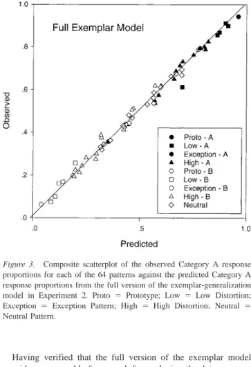
To gain a sense of the absolute fit of the exemplar model, in Figure 3, we present a composite scatterplot of the observed

Category A response proportions for each of the 64 patterns against the predicted Category A response proportions. Note that although the model was fitted to each individual subject’s data, in this composite plot the observed and predicted proportions are computed by averaging across the results from the 40 observers. Inspection of the composite plot indicates that the exemplar model is achieving accurate quantitative predictions of the data. Another indication of the model’s performance is that it accounted for an average of 87.0% of the response variance in the Category A response probabilities of the 40 individual observers. Likewise, the prototype model accounted for an average of 86.7% of the re-sponse variance.

Table 3

Maximum-Likelihood Fits (in Terms of⫺ln L) of the Models to the Classification Transfer Data Obtained in Experiment 2

Sub. Full proto. Full exemplar 3D-exemplar 2D-exemplar 1D-exemplar Matching exemplar

1 22.787 22.825 22.866 23.240 31.112* 42.479 2 13.235 13.407 13.407 13.591 16.040 41.964 3 37.354 37.354 37.354 37.477 42.147 78.951 4 75.470 75.148 75.580 78.006 90.969* 77.344 5 10.288 10.548 13.820 89.022* 140.568* 83.243 6 60.347 60.797 61.285 61.632 62.272 60.863 7 17.595 17.595 17.595 17.595 17.698 83.783 8 32.500 28.695 28.695 29.547 32.783 43.049 9 56.614 58.393 100.382* 108.341* 120.271* 65.844 10 24.516 26.130 26.411 27.510 28.365 81.170 11 44.617 44.641 44.983 47.976 53.480* 74.300 12 53.302 53.322 54.863 55.627 59.107* 69.630 13 16.406 16.447 16.658 16.716 17.698 41.303 14 43.607 43.489 43.489 43.605 44.497 48.237 15 4.709 4.829 6.192 7.546 8.924 40.154 16 44.950 44.698 45.001 46.843 48.340 75.713 17 81.402 82.550 82.688 83.567 84.517 82.927 18 22.904 22.911 23.127 23.431 24.509 42.423 19 33.533 33.534 33.534 36.518 44.422* 76.736 20 32.048 32.453 32.453 32.618 32.783 45.282 21 41.236 40.541 40.763 41.158 42.147 47.555 22 62.439 62.447 63.012 63.427 64.611 74.726 23 75.583 73.557 73.557 73.602 77.025 73.837 24 74.514 74.736 74.736 78.805 84.443* 77.979 25 68.948 68.627 68.627 70.898 104.535* 70.995 26 15.262 16.810 17.421 18.644 20.132 83.166 27 7.529 6.127 6.127 6.127 8.924 40.053 28 31.709 32.039 33.318 34.236 37.295 44.976 29 54.792 39.150 39.469 46.162* 144.577* 46.682 30 51.627 51.588 52.832 56.729* 81.759* 72.274 31 53.422 54.697 65.868* 84.268* 106.939* 72.372 32 42.795 41.643 41.797 50.832* 66.528* 48.136 33 62.886 63.362 63.866 64.247 64.992 76.842 34 11.715 11.893 11.893 12.427 15.059 40.964 35 20.982 22.298 22.836 24.423 26.495 41.953 36 39.647 37.456 38.792 39.942 42.332 44.852 37 81.341 81.374 85.218 105.014* 127.082* 94.153 38 50.385 50.445 53.615 69.014* 91.341* 64.784 39 48.500 48.533 48.554 49.081 50.787 50.773 40 6.127 4.709 4.710 6.127 8.924 85.118 Mean 40.741 40.295 42.185 46.889 56.661 62.690

Note. Sub.⫽Subject no.; Full proto.⫽Full version of the multiplicative-prototype model; Full exemplar⫽ Full version of the exemplar model; nD-exemplar⫽n-dimensional restricted versions of the exemplar model;

Matching exemplar⫽restricted version of the exemplar model with␥⫽1. Asterisks denote cases in which the

n-dimensional restricted versions of the exemplar model fit significantly worse than does the full version.

Having verified that the full version of the exemplar model provides a reasonable framework for analyzing the data, we now proceed to the tests of the restricted attention models. We fitted three different restricted versions of the model. In the first (1D-exemplar), we constrained the model such that all attention weight was given to a single dimension, with zero attention weight given to the remaining dimensions. In the second (2D-exemplar), we constrained the model such that all attention was split between two dimensions; and in the third (3D-exemplar), all attention was split among three dimensions. For simplicity in deriving the model fits, the dimensions that received attention were always those dimen-sions that had received the highest attention weights when the full version of the model was fitted to the data. These dimensions differed for each individual subject.

To test whether the restricted models provided significantly worse fits to each individual subject’s data than did the full model, we used the method of likelihood-ratio testing (Wickens, 1982). Let ln L(F) denote the log-likelihood of the data when the full model is fitted to the data, and let ln L(R) denote the log-likelihood fit of the restricted model. Assuming that the restricted model is correct, then the statistic G2 _{⫽ ⫺}

2 [lnL(R) ⫺ lnL(F)] has an approximate chi-square distribution with degrees of freedom equal to the number of parameters constrained in moving from the full to the restricted model.4

If the observed value of G2

exceeds the critical value, then one rejects the restricted model as fitting significantly worse than does the full model and concludes that at least some of the parameters were constrained inappropriately. We set alpha at .05 in conducting these tests.

The log-likelihood fits from the various restricted-attention ex-emplar models are reported along with those of the full exex-emplar model in Table 3. We denote with asterisks those cases in which the G2

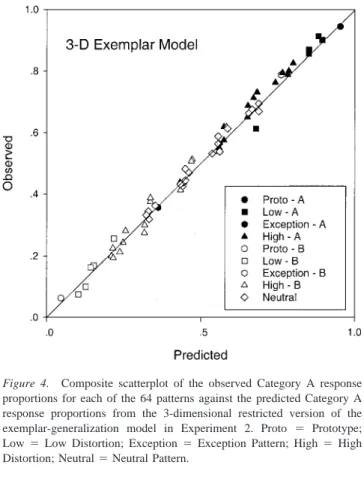
likelihood-ratio test leads one to reject the restricted model compared to the full model. For 25 of the 40 subjects, a single-dimension exemplar model, that is, a version of the exemplar model in which attention is given to only a single dimension, provides an adequate account of the data, that is, it is not rejected relative to the full version of the model. For 32 of the 40 subjects, the two-dimension version of the model is adequate, and for 38 of the 40 subjects, the three-dimension version is adequate.

To provide a better sense of these results, in Figure 4 we present the composite predictions from the three-dimension version of the model. Note that this model assumes that each subject attends to a maximum of three dimensions—for most of the subjects, almost all of the attention weight is placed on either one or two dimen-sions. Inspection of the composite scatterplot suggests that the low-dimension versions of the exemplar model are indeed provid-ing an excellent account of the individual subjects’ classification data.

Finally, in the last column of Table 3, we report the fits from the matching version of the exemplar model in which the response-scaling parameter is constrained at␥⫽1, with all other parameters allowed to vary freely. Not surprisingly, as was found by Smith et al. (1997; Smith & Minda, 1998), the matching model provides relatively poor fits to the classification data of the individual subjects. Indeed, its fits are often even worse than those of the highly constrained single-dimension exemplar model. The reason for these poor fits is that the matching model is unable to capture the levels of deterministic responding exhibited by many of the individual subjects. To gain another sense of the importance of the ␥ response-scaling parameter, we examined the maximum-likelihood parameter estimates from the fits of the full version of the exemplar model. This analysis revealed that 39 of the 40 observers had␥estimates greater than 1, with the median estimate being␥⫽4.77.

Discussion

In summary, the exemplar model provides an excellent account of the classification data observed at early stages of learning in the Smith et al. (1997; Smith & Minda, 1998) experimental paradigm, as long as the␥response-scaling parameter is allowed to vary. The fits of the exemplar model are essentially the same as those of the prototype model, which contains an implicit ␥response-scaling parameter. Nosofsky and Johansen (2000) reported similar results when they re-analyzed some of the individual subject data from Smith et al.’s (1997) study.

In addition, the results of the present analyses provided evidence consistent with the idea that numerous individual observers were

4_{A technical issue regarding the number of constrained parameters in} the restricted-attention models is that we do not specify a priori which dimensions receive zero weight. Nevertheless, we assume that the differ-ence in the number of freely varying attention weights used in the two models being compared provides a good approximation to the degrees of freedom in the chi-square test. Additionally, in all of our model-fitting procedures, we set upper limits on the sensitivity and response-scaling parameters of c⫽100 and␥⫽100.

Figure 3. Composite scatterplot of the observed Category A response proportions for each of the 64 patterns against the predicted Category A response proportions from the full version of the exemplar-generalization model in Experiment 2. Proto ⫽ Prototype; Low ⫽ Low Distortion; Exception ⫽ Exception Pattern; High ⫽ High Distortion; Neutral ⫽ Neutral Pattern.

attending selectively to a small subset of the dimensions compos-ing the objects. At early stages of learncompos-ing, subjects are not forming broad-based prototypes in this paradigm. The low-dimension rules that are being formed are equally well captured by versions of the exemplar and prototype models that assume selec-tive attention to just a few dimensions and that make allowance for the operation of deterministic response strategies. Contrary to the claims of Smith et al., the behaviors of subjects during the early-learning stages of this paradigm do not discriminate between the predictions of exemplar and prototype models.

Experiment 3

The central goal of Experiment 3 was to develop strong con-trasts between the predictions from the exemplar-generalization model and the mixed-prototype model advanced by Smith et al. (1997; Smith & Minda, 1998, 2000). Whereas in Experiment 2 we tested transfer performance after only four blocks of training trials, in Experiment 3 we conducted the transfer tests following 16 blocks of training. Smith et al. (1997; Smith & Minda, 1998, 2000) have acknowledged that following extensive training on a fixed set of items, memories for individual exemplars do play an important role in classification. However, they argued that the prototype representation continues to serve as the fundamental organizing principle of the category representation. The memories for the individual exemplars that are created are presumed to be all-or-none in the sense that they do not support any generalizations to new items. Such generalizations are presumed to be based on similarity to the prototypes.

Although Smith et al. (1997; Smith & Minda, 1998) demon-strated that this mixed-prototype model provided good accounts of classification performance at late stages of training, a limitation of their studies was that new transfer items were not included in the experimental designs. Rather, these researchers tested the ability of the mixed model to predict classification performance on only the old training items themselves. However, a major distinction be-tween the exemplar-generalization model and the mixed-prototype model rests on these models’ predictions of generalization to new transfer items. The exemplar model predicts that generalization is based on similarities to the stored exemplars, whereas the mixed-prototype model predicts that generalization is based on similarity to the prototype.

The prototype-plus-exception structure (see Table 1) designed by Smith et al. (1997; Smith & Minda, 1998) seems ideally suited for contrasting these models, as long as new items are included in the transfer tests. Specifically, consider new items that are similar to the old exception patterns that are stored in memory (i.e., Patterns 7 and 14 in the Table 1 structure). Because its exemplar-memory process is all-or-none, the mixed-prototype model tends to predict that such new items will be classified into the opposite category to which each exception belongs. That is, such new items will be classified in accord with the prototype structure of each category. By contrast, the exemplar-generalization model tends to predict that such new transfer items will be classified into the same category to which the respective exceptions belong. Although the precise predictions from the models depend on their parameter settings, the complete set of transfer stimuli provides multiple constraints such that the models cannot stray very far from the qualitative contrast outlined above.

Method

Subjects. Forty-three Indiana University undergraduates participated to partially fulfill a requirement of an introductory psychology class. Once again, we paid a bonus of $15 to the 2 subjects who achieved the highest accuracy in the experiment. None of the subjects had participated in the previous experiments.

Stimuli. The stimuli were the same as those used in Experiment 2.

Procedure. The procedure was identical to the one used in Experi-ment 2 except that in the current experiExperi-ment, subjects trained on a total of 16 blocks of the training stimuli (instead of the four blocks in the previous experiment).

Results and Theoretical Analysis

Model-based analyses of the learners’ data. Because the fun-damental contrast between the exemplar-generalization model and the mixed-prototype model pertains only to those observers who learned the training structure, we focus our main analyses on those observers who achieved over 86% correct on the training items during the transfer phase. (Even if an observer responds perfectly to the prototypes and low distortions, this criterion can be achieved only if he or she makes at least one correct response for an exception item.) Twenty-two of the 43 subjects met this learning criterion. We report the modeling analyses for the nonlearners in a later section.

We fitted the exemplar-generalization model and the mixed-prototype model to the classification transfer data obtained for each of the 22 learners by using a maximum-likelihood criterion.

Figure 4. Composite scatterplot of the observed Category A response proportions for each of the 64 patterns against the predicted Category A response proportions from the 3-dimensional restricted version of the exemplar-generalization model in Experiment 2. Proto ⫽ Prototype; Low⫽Low Distortion; Exception⫽Exception Pattern; High ⫽High Distortion; Neutral⫽Neutral Pattern.

The log-likelihood fits for each of the models are reported in Table 4. As an auxiliary measure, we also report the percentage of variance in the Category A response probabilities that is accounted for by each model. The exemplar-generalization model provides a better log-likelihood fit than does the mixed-prototype model for 18 of the 22 learners. In a large number of cases, the improved fit provided by the exemplar-generalization model compared with the mixed-prototype model is quite dramatic. In no case does the mixed-prototype model provide a substantially better fit than does the exemplar-generalization model. Across the 22 learners, the log-likelihood value achieved by the exemplar-generalization model (mean ⫺ln L ⫽ 33.9) is significantly better than that achieved by the mixed-prototype model (mean ⫺ln L ⫽ 51.9),

t(21)⫽3.89, p⬍.001. The percent variance measure shows the same pattern of results.

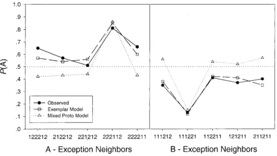
It is instructive to consider the patterns of classification transfer data to gain an understanding of the reason for the better perfor-mance of the exemplar-generalization model compared to the mixed-prototype model. In the following analysis, we define the “neighbors” of exception-training Exemplars 7 and 14 as those novel transfer stimuli that differ from the exceptions along only a single dimension value. In general, the exemplar model tends to predict that the neighbors will be classified into the same category as the exception to which they are similar, whereas the mixed-prototype model tends to predict the opposite. The results for each

of the neighbors, averaged across the observed and predicted classification probabilities from all 22 learners, are displayed in Figure 5. As can be seen, the exemplar model predicts well the classification probabilities for the neighbors. By contrast, the pat-tern of results is qualitatively inconsistent with the predictions from the mixed-prototype model. For both the Exception 7 neigh-bors and the Exception 14 neighneigh-bors, in four of five cases the mixed-prototype model predicts that these transfer stimuli will be classified into the opposite category from what was actually ob-served. (The reason that the mixed-prototype model predicts cor-rectly the results for Transfer Stimuli 222112 and 111221 is that many subjects gave a good deal of attention weight to Dimensions 4 and 5. Transfer Stimuli 222112 and 111221 happen to match the corresponding prototypes on these particular dimensions.)

We emphasize that the summary results illustrated in Figure 5 are based on averaged data. Providing a full explanation of the pattern of results requires a specification of how individual ob-servers distributed attention across the dimensions of the stimuli. We conducted additional analyses in which the neighbors were defined for each individual observer based on the particular di-mensions that he or she attended. In these individual observer analyses, the superiority of the exemplar model over the mixed-prototype model was often even more pronounced than is illus-trated by the composite plot in Figure 5.

Recall that Smith et al. (1997; Minda & Smith, 2001; Smith & Minda, 1998) compared the mixed-prototype and exemplar-generalization models on their ability to fit the classification pro-portions associated with the training stimuli only. It is instructive to point out that had we followed this procedure, it would have yielded far less dramatic differences in quantitative fit between the models. When we fitted the models to the data from only the training instances, in 10 of 22 cases the mixed-prototype model gave slightly better log-likelihood fits than did the exemplar model, although the mean ⫺ln L for the exemplar model (2.66) was still significantly smaller than that of the mixed-prototype model (3.51), t(21)⫽2.82, p⬍.05. Both models yield extremely good fits for an uninteresting reason: As training proceeds, ob-servers learn to classify all of the old instances with essentially perfect accuracy. The mixed-prototype model fits such perfor-mances simply by setting its exemplar-memory parameter e at a value near 1. Thus, testing the ability of the mixed-prototype model to generalize to new transfer stimuli is crucial for evaluating the utility of this model.

Model-based analyses of the nonlearners’ data. For complete-ness, we also fitted the exemplar-generalization and mixed-prototype models to the data of the 21 observers who failed to meet the learning criterion. The model fits are reported in Table 5. With the exception of a few observers, there was little difference in the quantitative fits of the two models. The exemplar-generalization model provided a better fit for 11 of the 21 nonlearners, and its average log-likelihood fit (⫺ln L⫽47.1) was slightly better than that of the mixed-prototype model (⫺ln L⫽51.4). However, the differences in the log-likelihood fit values were not statistically significant, t(20)⫽1.52, p⬎.10. In general, the behavior of most of the nonlearners was similar to those subjects from Experiment 2 who were trained on only four blocks of training trials. Because these subjects often focused attention on a single dimension, or on a small number of dimensions that were not perfectly diagnostic of category membership, they failed to learn to classify all of the Table 4

Summary Fits of the Multiplicative-Prototype Model, the Mixed-Prototype Model, and the Exemplar-Generalization Model to the Learners’ Transfer Data From Experiment 3

Sub.

Prototype Mixed Exemplar

⫺ln L % Var ⫺ln L % Var ⫺ln L % Var

1 91.783 49.6 84.117 54.5 7.591 99.2 2 102.451 35.8 97.339 42.7 62.794 75.1 3 34.692 92.0 34.670 92.1 28.012 94.9 4 57.014 74.0 46.060 80.8 24.200 94.7 5 53.346 81.7 47.949 85.2 39.629 89.3 6 83.009 53.3 76.558 59.3 36.151 88.7 7 42.104 86.7 40.610 87.5 38.426 88.7 8 51.703 79.3 51.400 80.0 31.928 93.1 9 49.444 76.6 47.366 77.5 36.280 83.3 10 31.333 89.6 17.168 95.0 20.555 94.5 11 41.712 84.3 26.577 92.6 27.754 90.8 12 68.536 69.2 54.338 79.4 30.188 95.4 13 73.981 66.6 61.456 74.2 46.579 86.0 14 34.893 91.7 31.384 93.0 31.739 91.9 15 85.175 54.9 75.797 60.6 59.431 74.8 16 60.435 76.4 57.448 79.4 51.634 81.9 17 54.090 80.5 49.076 83.2 39.352 91.0 18 43.386 83.9 42.913 84.2 44.304 83.2 19 96.159 52.8 82.610 59.4 10.813 98.7 20 14.017 98.2 13.974 98.3 13.694 98.3 21 46.473 78.8 44.532 80.7 34.532 91.3 22 68.012 63.2 58.964 71.6 30.435 94.0 M 58.352 73.6 51.923 77.8 33.910 90.0

Note. Smaller values of⫺ln L reflect a better fit of a model. Sub.⫽ Subject no.;⫺ln L⫽negative log-likelihood; % Var⫽percentage of variance accounted for; Prototype⫽Prototype model; Mixed⫽ Mixed-prototype model; Exemplar⫽Exemplar-generalization model.