Bayesian Sensitivity Analysis for Non-ignorable Missing Data in Longitudinal Studies

(1)

Bayesian Sensitivity Analysis for

Non-Ignorable Missing Data in

Longitudinal Studies

by

Tian Li

B.Sc., University of Manchester, 2014

Project Submitted in Partial Fulfillment of the Requirements for the Degree of

Master of Science in the

Department of Statistics and Actuarial Science Faculty of Science

c

• Tian Li 2017

SIMON FRASER UNIVERSITY Spring 2017

Copyright in this work rests with the author. Please ensure that any reproduction or re-use is done in accordance with the relevant national copyright legislation.

(2)

Approval

Name: Tian Li

Degree: Master of Science (Statistics)

Title: Bayesian Sensitivity Analysis for Non-ignorable Missing Data in Longitudinal Studies

Examining Committee: Chair: Jinko Graham

Professor

Lawrence McCandless

Senior Supervisor Associate Professor Faculty of Health Sciences &

Associate Member

Statistics and Actuarial Science

Joan Hu Supervisor Professor Julian Somers Internal Examiner Associate Professor Faculty of Health Sciences

(3)

Abstract

The use of Bayesian statistical methods to handle missing data in biomedical studies has become popular in recent years. In this thesis, we propose a novel Bayesian sensitivity analysis (BSA) model that accounts for the influences of missing outcome data on the estimation of treatment effects in randomized control trials with non-ignorable missing data. We implement the method using the probabilistic programming language Stan, and apply it to data from the Vancouver At Home (VAH) Study, which is a randomized control trial that provided housing to homeless people with mental illness. We compare the results of BSA to those from an existing Bayesian longitudinal model that ignores missingness in the outcome. Furthermore, we demonstrate in a simulation study that, when a diffuse conservative prior that describes a range of assumptions about the bias effect is used, BSA credible intervals have greater length and higher coverage rate of the target parameters than existing methods, and that sensitivity increases as the percentage of missingness increases.

Keywords: Bayesian methods; longitudinal analysis; missing data; sensitivity analysis; Simon Fraser University; Vancouver At Home study

(4)

Dedication

This thesis is dedicated to all my friends, including (in alphabetical order of the last letter of the surname)

Sarshar Hosseinnia Sagar Mehta Hassan Kulmie Vasilis Se Hossein Sharifi Qingyuan Feng Kenneth Chung Lillian Y L. Michael McGovern Angel Granados

Michael James Rogers Angus Lockhart

Jaypratap Naidu

who have laughed, wept, walked, run and played FIFA with me over the years, and from whom I have learnt far more than I could ever have hoped for.

(5)

Acknowledgements

I would like to express my utmost gratitude to the following individuals and organization: my supervisor, Professor Lawrence McCandless, for the conception of this thesis and for his guidance, support and inspiration throughout my MSc career at SFU that culminated in this final piece of work, which would not have been presentable without his important suggestions and edits,

the examining committee members,Professor Joan Hu,Professor Julian Sommers

and Professor Jinko Graham, for their time, patience and insightful feedback,

the creators of R, Dr. Robert Gentleman and Professor Ross Ihaka, andmany other contributors, for developing such an amazing statistical language,

the founder of RStudio, J. J. Allaire, and the RStudio team, for making it so much easier to code in said language,

and last but not least, my parents,Chunling Wang andYuexue Li, for unreservedly supporting everything I do.

(6)

List of Tables

Table B.1 Descriptive statistics of the Vancouver at Home dataset of n=297 home-less individuals with mental illness . . . 41 Table B.2 Number of participants at baseline and each revisit . . . 41 Table B.3 QoL mean scores at baseline and 6, 12, 18 and 24 months followup by

study arm . . . 41 Table B.4 Posterior mean and 95% HPD credible interval of variables in a

tra-ditional Bayesian longitudinal model that ignores missing data (naïve model) . . . 43 Table B.5 Posterior mean and 95% HPD credible interval of overall treatment

effect for βvm = {-30, -20, -10, 0, 10, 20, 30} with varied γ0 andγx . . 44

Table B.6 Posterior mean and 95% HPD credible interval of model parameters for Bayesian sensitivity analysis (BSA) applied to the At Home data using a uniform (-30, 30) prior distribution on the bias parameter βvm 44

Table B.7 Coverage and length of 95% HPD credible intervals for the naïve and BSA methods obtained from the simulation study . . . 44

(9)

List of Figures

Figure B.1 Group allocation of high needs participants in the At Home study 40 Figure B.2 Average QoL trajectories in HF and TAU groups . . . 42 Figure B.3 Individual QoL trajectories for a random sample of size 30 generated

from the HF group . . . 42 Figure B.4 Individual QoL trajectories for a random sample of size 30 generated

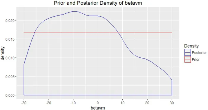
from the TAU group . . . 43 Figure B.5 Prior and posterior density ofβvmobtained using Bayesian

(10)

Chapter 1

Introduction

In longitudinal studies, repeated observations of the same subjects are taken over a period of time. In an ideal world, researchers would be able to monitor every subject at every scheduled point. However, just as most things in life, studies do not always go according to plan and missing observations to various extents do occur against the best wishes of everyone involved.

Numerous methods have been devised to deal with the issue of missing data [8][16][17][28]. In this thesis, we propose a novel Bayesian sensitivity analysis (BSA) specifically for non-ignorable missing data, also known as missing not at random (MNAR) data, and apply this method to data obtained from a study.

In the rest of this chapter, we conduct a review of different types of missing data and their occurrence in longitudinal studies, as well as existing methods in the literature for sensitivity analysis of MNAR data. Chapter 2 discusses an example of a real life longitudinal study with such a problematic type of missing data. It concerns a randomized controlled trial that provided housing to homeless people with mental illness from Vancouver (Patterson et al. [25]). In Chapter 3 we review an existing standard Bayesian random effects model that ignores missing data, which can be compared to the novel BSA method we introduce in Chapter 4. Chapter 5 details a simulation study on the performance of the new method in comparison with the existing method. Discussions are presented in the last chapter.

1.1

Review of Missing Data

Missing data are a common occurrence in research in vast majority of scientific disciplines [8]. Governments, firms and organizations may withhold or fail to report key statistics of

(11)

national or commercial interest, which is mostly applicable to studies in social sciences [23]. When data are collected using surveys and interviews, non-response may be a cause of concern, where participants fail to respond to one or more items, or an entire survey altogether (although such cases can be safely ignored) for various reasons. Questions on certain subjects of a private nature, such as level of income, may elicit a higher rate of non-response in a particular group of participants [33].

Missingness may also be inadvertently caused by researchers in the form of human errors, as a consequence of mistakes in data collection and data entry [1]. Nevertheless, this type of missing data can be relatively easy to rectify if the original measurements or observations are available.

Various problems can arise due to missing data. A significant lack of data translates to a reduction in sample size and lower statistical power than intended. In addition to complicating otherwise straightforward statistical analyses, incomplete data may also cause bias in the estimation of model parameters, potentially rendering the conclusions invalid [32]. Bias can occur when the observed data are not representative of the entire population under study, for example, when study participants that have complete observations are healthier and more affluent than the others.

1.2

Missing Data in Longitudinal Studies

Missing data are a critical issue in longitudinal studies. In fact, it has been said that “in longitudinal studies in health sciences, missing data are the rule, not the exception” [10]. The most common type of missingness here is attrition, or dropout. As the name implies, such incidents take place when participants drop out of the study before its completion, resulting in missing observations.

The choice of methods for handling missing data in longitudinal studies is primarily dependent on the pattern and mechanism of missingness, which we outline in the following subsections.

1.2.1 Patterns of Missing Data

Two patterns of missing data exist in longitudinal studies. A monotone missing pattern occurs when a study participant is absent for measurement or observation at a particular point and all points afterwards [17]. That is, once they fail to show up, they are never heard from again.

(12)

On the other hand, data are non-monotone missing, or intermittent missing, if obser-vations on a participant are made after they miss a previous data collection point [17]. It is possible that they become missing again, either temporarily or permanently. These participants are not technically considered dropouts since they did not leave of the study forever at the first instance of absence.

In reality, a strictly monotone missing pattern is an uncommon occurrence [16], since it is unlikely that all participants would be able to adhere to the study schedule without missing any intermittent points due to personal or other reasons.

1.2.2 Classification of Missing Data

In a landmark paper on missing data [27], Rubin classifies them into three categories, missing completely at random (MCAR), missing at random (MAR) and neither. The last category was later named as missing not at random (MNAR) [28].

Data are MCAR if the probability of failing to observe a value is independent of any observed or unobserved values of the response variable, or any other observed values [28]. A hypothetical example could be that, in a study on the effect of diet on cholesterol level, participants roll a dice to decide whether to attend a measurement session. Under the MCAR assumption, the observed data can be considered as a random sample of the complete data and there is no bias in the parameter estimates.

Data are said to be MAR if the probability of failing to observe a value is independent of any unobserved values of the response variable, but dependent on observed values of the response variable or some other variables [28]. In this regard, it is perhaps more intuitive to interpret this type of data as “missing conditionally at random”. In our hypothetical study, MAR would occur if participants with a lower measured cholesterol level in a session are more likely to miss subsequent sessions, or if participants on a specific type of diet are more inclined to be absent.

By definition, if data are MCAR, they are also MAR [4]. Both MCAR and MAR are ignorable within the likelihood and Bayesian frameworks, whereas in frequentist framework, ignorability is only applicable to MCAR [27].

When the probability of failing to observe a value is dependent on the missing value itself, it is known as MNAR, or informative missing [28]. Failure of participants to turn up for a session in the cholesterol study should be attributed to MNAR provided that the missingness is related to their cholesterol level in that very session, MNAR is non-ignorable

(13)

because there is no information on the influence of the missing data, requiring the missing mechanism to be modelled. Treatment of MNAR data is the focus of this thesis.

It is very difficult to ascertain the missing data mechanism in any given study, al-though several methods have been developed to test for MCAR assumption by Little [22], Listing and Schlittgen [20][21] and Diggle [7], among others. Enders [8] discusses two pro-cedures that distinguish between MCAR and MAR, which rely on the assessment of the independence of the missing indicator and the observed covariates using tools such as lo-gistic regression. Notwithstanding, in general there is no way to determine whether MAR or MNAR exists for they rely on information that is missing, unless follow-up data are obtained from non-respondents for verification [29].

1.3

Review of Existing Methods in the Literature for

Sensi-tivity Analysis of MNAR Missing Data

Popular and well-documented methods for handling missing data include multiple im-putation, maximum likelihood estimation, complete case analysis and Bayesian methods [17]. Application of these methods to MNAR data requires specification of the missing data mechanism, which calls for the use of sensitivity analysis to assess the sensitivity of model-based inferences to the unverifiable MAR assumption.

Limited resources on sensitivity analysis for non-ignorable missing data in longitudinal studies exist in the statistical literature, probably as a consequence of the highly speculative nature of such analyses. Of those available, the textbook of Daniels and Hogan [6] describe the procedures applied to two longitudinal studies.

The first example is the Growth Hormone study conducted by Kiel et al. [19]. It is a controlled trial of longitudinal data that investigates the effect of growth hormone and exercise on changes in quadriceps strength, with missing outcome data. Daniel and Hogan [6] limit the discussion to two study arms, exercise plus placebo versus exercise plus growth hormone. In a similar approach to ours (to be introduced later), they construct a pattern mixture model with a large number of sensitivity parameters, which are eventually reduced to a subset of the intercept sensitivity parameters that are allowed to vary in order to account for the deviation from the MAR assumption [6]. Subsequently they carry out a sensitivity analysis examining the posterior inferences about the treatment effect by summarizing the posterior mean and posterior probability over a domain that is calibrated with relevant posterior distributions under MAR.

(14)

The second example described by Daniels and Hogan [6] concerns the OASIS trial. This was a randomized controlled trial that compared the effect of standard versus enhanced counselling interventions on smoking cessation rates among alcoholics, with missing binary outcomes. Daniel and Hogan fit both parametric selection models and pattern mixture mod-els with elicited informative priors on the odds ratio at each stage of assessment. Departure from MAR was realized by defining a pair of log odds ratio parameters. They concluded that sensitivity analysis was inappropriate in the case of parametric selection models due to identifiability and that the pattern mixture models fit well because of easily separable parameter space [6].

Elsewhere in the literature, Kenward [18] pedagogically illustrates the use of a sensi-tivity analysis to examine the effect of the distributional assumptions on the estimation of dropouts using the outcome-based selection model proposed by Diggle and Kenward [7]. In a later paper, Verbeke et al. [35] presents a local influence approach based on the work of Diggle and Kenward to sensitivity analysis for MNAR data, adopted on the concept of individual-specific infinitesimal perturbations around the MAR model. It involves the assignment of a perturbation within the linear predictor of the model to the potentially unobservable measurements.

A different strain of the local influence approach is proposed by Ganjali and Rezaei [12], who utilize a generalized Heckman model to assess the influence of a small perturbation of elements of the covariance structure on the likelihood. It functions as a global sensitivity analysis for cross-sectional and longitudinal data with two periods. The authors suggest the use of normal curvature for longitudinal data with more periods.

Troxel et al. [34] propose a measure of local sensitivity based on a Taylor series ap-proximation to the non-ignorable likelihood, evaluated at the parameter estimates under the ignorability assumption. An index of sensitivity to non-ignorability is derived from the approximated likelihood, which allows researchers to evaluate the need for more elaborate sensitivity analysis or MNAR modelling.

(15)

Chapter 2

Data Example

To motivate our discussion of missing data in longitudinal studies, we consider the dataset described by Patterson et al. [25]. The data concern 297 homeless people from Vancouver, British Columbia who participated in the Vancouver At Home (VAH) Study between 2009 and 2013. The VAH Study was a randomized control trial in which homeless participants with mental illness were randomly allocated to receive housing with supports (treatment) or no housing (control), and then followed prospectively to collect information about health outcomes and service use with repeated measurements over time [31].

2.1

Background: Homelessness in Canada and the At Home

/ Chez Soi Study

Over the last three decades, homelessness has emerged to be one of the most prominent social issues in Canada [36]. According to the Canadian Observatory of Homelessness, it is defined as “the situation of an individual or family without stable, permanent, appropriate housing, or the immediate prospect, means and ability of acquiring it” [2]. A report by the same organization estimates that in 2016, at least 235,000 Canadians were subject to homelessness at some point during the previous year and that 35,000 Canadians were homeless on any given night [11]. In particular, as one of the largest cities in Canada, Vancouver too has seen a steadily growing population of homeless individuals, most of whom are concentrated in Downtown Eastside [5]. As of 2011, 2650 people experienced homelessness in Metro Vancouver, compared to 1121 in 2002 [15].

Studies have demonstrated that homeless people are particularly susceptible to mental illnesses [9] and substance addiction [24], which doubtlessly have detrimental effects on

(16)

their already difficult and stressful circumstances. Many of these vulnerable individuals are unable to receive adequate healthcare and social support due to limited funding and investments in community-based mental health programs and affordable housing [14].

To combat homelessness, many policy experts recommend a “Housing First” approach. Housing First provides homeless people with immediate access to subsidized housing, to-gether with supports [14]. No pre-conditions, such as bringing substance abuse under control or being stabilized on medications are imposed. The premise of Housing First is that people should be more capable of moving forward with their lives if they are first provided with housing.

To better understand the impact of a Housing First approach to tackling homelessness in a Canadian context, in 2008 the Mental Health Commission of Canada undertook a $110 million national study called the At Home / Chez Soi Study [36]. This project recruited 2500 participants over four years in five Canadian cities, namely Moncton, Montreal, Toronto, Vancouver and Winnipeg.

2.2

The Vancouver at Home (VAH) Dataset

For this MSc thesis, we will analyze data in the VAH Study that covers specifically the city of Vancouver. In other words, we will focus on data from the Vancouver portion of the nationwide At Home / Chez Soi Study. A complete description of the study protocol is given by Somers et al. [31].

We consider a dataset consisting of the n= 297 high-needs (HN) homeless individuals participating in the VAH. Participants were 19 years of age or older, and homelessness was defined as having no fixed place to sleep for more than 7 nights with little likelihood of obtaining accommodation. High need individuals, as defined by Somers et al. [31], had severe mental illness combined with criminal justice involvement, substance dependence or other factors.

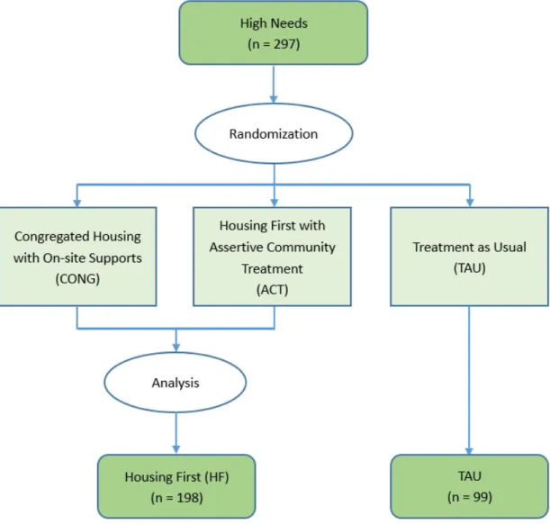
In the VAH Study, the 297 participants were randomly assigned to one of three study groups:

1) Independent Housing First with Assertive Community Treatment, which consisted of scattered subsized rental housing around the city

2) Congregate Housing First, where all participants were housed together in a single building in downtown Vancouver, or

(17)

People in the TAU group received no further housing or support services from the study apart from the existing services for homeless individuals with mental illnesses in Vancouver. The participants were randomly assigned to the three treatment groups and then fol-lowed prospectively for up to two years. See Figure B.1 for a diagram of the treatment assignment. Data were collected by interview, and each participant was interviewed up to 5 times: once at baselined prior to randomization, then then up to four more times at 6-month intervals.

Several study hypotheses were formulated, among which was that Housing First would have a positive influence on the quality of life (QoL) of the homeless individuals with mental illness as compared to TAU. Thus, the dependent variable in our analysis was the QoL score (see below for details).

The previous analysis by Patterson et al. [25] concluded that the QoL of participants in HF improved significantly more than that of participants in TAU at both 6 and 12 months post baseline. Still, an important potential limitation was that a small proportion of study data was missing as some participants failed to attend one or more scheduled interviews. We are unable to ascertain its impact on the results, especially as participants in TAU were established to be more likely to drop out of the study.

2.3

Basic Descriptive Statistics and Pattern of Missing Data

The objectives of this project are to examine the effects of missingness in the response variable, QoL scores, in the VAH study, and additionally to develop an effective method to explore the sensitivity of analysis results to missing data.

Before conducting any analyses, we begin with the simplifying assumption that the first two Housing First treatment groups (scattered-site housing versus congregated housing) are merged into a single treatment group, which we henceforth call “HF” for Housing First, to facilitate comparison with the control group TAU. This is due to the consideration that the first two groups both involved the provision of housing and there were no statistically signif-icant differences in the measurements of QoL in both groups across the entire study period. Thus, we assume that there are only two arms in the randomized trial: HF (treatment) versus TAU (control). The limitations are discussed further in the Discussion (Section 6.1).

(18)

id A unique and de-identified id for participant

visit.number The visit number

visit.type A description of the visit type (baseline, 6 months etc.)

visit.date Month and year of visit

csi Colorado Symptom Index (see below)

qol Quality of life score (see below)

male Indicator variable, 1 if participant is male

age.ord Age as an ordinal variable with 3 categories

num.health.ind Total number of health conditions

hf Indicator variable, 1 if Housing First

total.num.visits Total number of visits

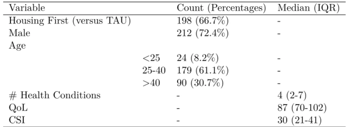
We begin with presenting the descriptive statistics of the baseline characteristics of the 297 participants in the study, as shown in Table B.1. A total of 198 (66.7%) individuals were allocated to the HF group and 99 (33.3%) to the TAU group. A total of 72.4% of the participants were male (n = 212), reflecting the actual predominance of males in the homeless population in Vancouver. The largest age group represented was 25-40 years of age (n = 179, 61.1%), followed by over 40 (n = 90, 30.7%) and below 25 (n = 24, 8.2%).

All participants were homeless with mental illness at baseline. Consequently, they had a median of 4 chronic health conditions (interquartile range (IQR) 2-7), which were defined as serious health problems such as diabetes that lasted longer than 6 months. The median Colorado Symptom Index (CSI) score was 30 (IQR 21-41). CSI is a continuous measure of mental health symptoms based on 14 questions with Likert scale 1-5 and higher values represent worse mental health. If more than 50% of the questions were completed, the remainder were imputed with the arithmetic average of the completed questions, otherwise the CSI scores were recorded as missing.

The dependent variable in this MSc thesis is QoL. The median QoL at baseline was 87 (IQR 70-102). The QoL metric adopted in the study was the Quality of Life Interview 20 (QOLI-20), which measures 20 subjective items in 6 subscales: family, finances, leisure, living situation, safety and social. Additionally, there is a global item that assesses an individual’s overall satisfaction with life. As some participants did not complete all 20 QoL questions, two approaches were used to handle the missing responses. If more than 50% of the questions were completed, the remainder were imputed with the arithmetic average of the completed questions. Otherwise their QoL scores were recorded as missing.

Table B.3 presents the mean QoL scores (standard deviation (SD)) in HF versus TAU at baseline and at the 4 subsequent 6-month visits. p-values to test for differences were calculated using a 2-sample t-test. As expected, there was no significant difference in the QoL at baseline (p = 0.8819) because the participants were randomly assigned to both

(19)

groups and HF cannot affect the outcome at baseline. However, significant differences were found for 6 months (p = 0.0028), 12 months (p = 0.0116) and a slightly weaker one for 24 months (p = 0.0808), indicating higher mean QoL scores in the HF group.

Figure B.1 shows the mean of the QoL trajectories in HF and TAU. It is clear that there is an increasing trend in both groups and the HF group sees a faster increase overall. However, an interesting curiosity is that the difference between the curves tends to diminish over time. Thus, although HF has a positive impact on QoL compared to TAU, the magnitude of the treatment affect appears to be greatest earlier in the follow-up period. The increase of the mean QoL score in TAU was also observed in Patterson et al. [25]. A likely explanation for this interesting finding is that the participants were in such poor health at the time of recruitment that their QoL scores improved even in the absence of provision of housing.

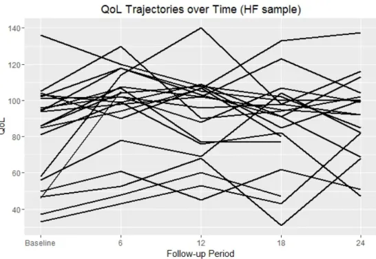
To illustrate the longitudinal nature of the data, Figure B.2 and Figure B.3 present in-dividual QoL trajectories for a random sample of 30 participants from both groups. Figures B.2 and B.3 illustrate the within-subject and between-subject variability in QoL scores over time.

An important concern in the VAH Study, which is the basis of this thesis, is missing data. All participants were scheduled to be interviewed a total of 5 times (baseline, 6, 12, 18 and 24 months). Although data were collected for all 297 at baseline, the number of participants that were revisited at 6 months was reduced to 270, which further declined to 264, 247, 231 at 12, 18 and 24 months, as shown in Table B.2. While a number of dropouts occurred, some individuals remained in the study but skipped one or more intermediate revisits.

Moreover, TAU participants were less likely to participate in follow-up interviews. Out of all QoL measurements at 4 revisits, 9.7% were missing in the HF group (n = 75). At 21.5%, the percentage of missingness in the TAU group is slightly more than twice that in HF. (n = 85). Clearly and unsurprisingly, participants that were not favoured by the god of probability in the random treatment assignment had little incentive to remain in the study because they did not get housing.

The key scientific question is therefore whether the excess loss to follow-up in the TAU group may have biased the analysis findings. For instance, if healthy TAU participants were less likely to be lost to follow-up, this could in theory bias the mean QoL trajectory curve in the TAU group and decrease the treatment effect. In effect, there would be a “selective attrition” where the TAU group comprised predominantly healthy individuals (with high QoL scores), which would describe a MNAR scenario. However, we have no way to confirm this as the available data cannot answer this question.

(20)

Chapter 3

A Longitudinal Analysis that

Ignores Missing Data in the

Outcome Variable Quality of Life

Recall that the data consists of longitudinal measurements of Quality of Life Scores in

n = 297 participants, who were followed prospectively for 24 months. Each participant was randomly allocated to either treatment (Housing First (HF)) or control (Treatment as Usual (TAU)). They were then interviewed up to 5 times (baseline, 6 months, 12 months, 18 months and 24 months), and detailed data were recorded. The dependent variable in the analysis was repeated measures of Quality of Life (QoL).

Previously, longitudinal data analyses of the VAH data were conducted in a paper by Patterson et al. [25]. The authors used a linear mixed effects regression to model the asso-ciation between the different types of HF and the normally distributed outcome QoL. In the regression analysis, the authors included time (discrete 6 month intervals) and interaction terms between time and study arm, which capture the treatment effects. Furthermore, in the multivariable model the authors adjusted for baseline covariates including age, gender and other variables such as housing status at baseline and duration of previous homeless-ness. Patterson et al. [25] found that HF was associated with significantly greater QoL scores as compared to TAU.

The statistical issue that motivates this research project is theintermittentmissing data of QoL measurements. As described in Chapter 2, participants assigned to TAU were less likely to be interviewed in the follow-up period because of a lack of incentive to participate in the study. Yet such missingness does not constitute loss to follow-up as some participants skipped one or more interviews but were interviewed again later in the study. The concern

(21)

here is then how this might have affected the results. For example, if TAU participants with worse health were more likely to be lost, the QoL trajectory in TAU may have been biased as a result of attrition of the sickest patients.

In this section of the thesis, we begin by replicating the linear mixed effects analysis of Patterson et al. [25] using Bayesian methods implemented in the software STAN. The analysis results will serve as a point of comparison with the subsequent analyses where we model the missing QoL score directly using a non-ignorable missing data model.

3.1

Model

Building upon the analysis of Patterson et al. [25], we present a Bayesian linear mixed effect models to account for correlation in repeated measures of QoL scores in the VAH Study. For ease of reference, this model will be named as the “naïve” model because it naïvely ignores the role of missing data in the analysis.

3.1.1 Variables and Notation

Let Yij be the quality of life score for ith participant in the jth record, where i = 1,2, . . . ,297and j= 1,2,3,4,5 represents baseline and first to fourth visit respectively.

LetXi be an indicator variable for the group allocation of theithparticipant, such that Xi = 1 ifith participant is in the HF group

= 0 ifith participant is in the TAU group

Note that in the VAH study the treatment allocation was fixed over time. Despite that, the TAU participants were not prevented from find housing on their own. Consequently, a limitation (discussed in Chapter 6) is that the TAU individuals might in fact have obtained housing through other means.

(22)

To model time (i.e. follow-up visit), for each participant in the jth record, we create a vectorfVj of length 4 to represent the number of visit, such that

f

Vj= [0,0,0,0]for baseline (0thvisit), = [1,0,0,0]for the first visit,

= [0,1,0,0]for the second visit,

= [0,0,1,0]for the third visit,

= [0,0,0,1]for the fourth visit.

Therefore the data consist of (Xi,fVj, Yij), where Xi and fVj are always observed, but

the outcome variableYij is sometimes missing for certain combinations ofiandjand those

missing values are simply ignored in this model.

3.1.2 Model for QoL that Ignores Missing Data (Naïve)

We present the naïve model here, which ignores missing data. The underlying assump-tion in this model is that the QoL score of each participant at any time is affected only by the group allocation and time of visit. We model Yij using the following linear mixed

effects model

Yij|Xi,fVj ∼N(θi+fVjTβev+ (VfjTβevx)Xi, σ2) (3.1)

for all pairs (i, j) such that Yi,j is observed. In the dataset there were 1305 QoL scores

available for analysis, although we would expect a total of 297×5 = 1485observations. In the model, the quantityθiis a random effect that can be interpreted as the mean QoL

score for individual i at baseline if they were assigned to TAU. We assign a model for the random effects asN(µθ, δ2θ), whereµθ captures the mean andδ2θ governs the heterogeneity.

The vector βev = [βv1, βv2, βv3, βv4] of time effects models how the mean of the QoL

trajectory changes over time in the TAU group. The vector βevx = [βvx1, βvx2, βvx3, βvx4]

consists of treatment-by-period interactions. Finally, σ is the residual standard deviation of the QoL scores that is not explained by the model.

For simplicity, Equation (3.1) does not include any covariates (e.g. age and gender) and in principle they could be easily added to the model.

(23)

The interactionβevxare the main target of inference in the analysis because they describe

the treatment effect. To illustrate, the expected QoL score for participants in the TAU group, marginalizing over the random effects θi, can be expressed as

E[Y|X = 0,fV] =µθ+fVT(βev) (3.2)

whereas the expected QoL score for participants in the Housing First group is given by

E[Y|X= 1,fV] =µθ+VfT(βev+βevx) (3.3)

Consequently, the vector of four treatment effects at times 6, 12, 18 and 24 months is then

E[Y|X = 1,fV]−E[Y|X= 0,fV] =VfT(βevx) (3.4)

Note that the treatment effect at time zero (baseline) is set to exactly zero in equation (3.1) since, by definition, when participants were assigned to treatment at time zero, the causal effect of treatment must be zero.

3.2

Prior Distributions

There are five parameters in the aforementioned model, namelyµθ, σ2θ,βev,βevx, σ2.

Fol-lowing Gelman et al. [13], the folFol-lowing priors were chosen for the parameters,

µθ ∼N(0,100) σ2_θ ∼N(0,100000)+ e βv ∼N        0,        100 0 0 0 0 100 0 0 0 0 100 0 0 0 0 100               e βvx∼N        0,        100 0 0 0 0 100 0 0 0 0 100 0 0 0 0 100               σ2 ∼N(0,100000)+

(24)

where N(a, b)+ is a normal distribution with mean a and variance b that is truncated to be strictly positive. An N(0,100) prior is assigned to the random effect, time effect and treatment by period interaction to reflect the realistic variation in QoL scores (in the range [20, 140] in the dataset). However, a diffuse prior N(0,100000) is used for the variances

σ_θ2 and σ2 due to a lack of prior information, indicating that a large range of values are plausible.

3.3

Computations Using Stan

Stan is a probabilistic programming language for Bayesian statistical inference [3]. Writ-ten in C++, it is used to specify statistical models and implements Markov Chain Monte Carlo (MCMC) methods, gradient-based variational Bayesian methods and gradient-based optimization for penalized maximum likelihood estimation. Stan is realized in R using the

rstanpackage.

In the analysis, we defined the list of data,

int n; (number of participants)

int nk; (number of data records)

int id[nk]; (vector of participant ids of length 5n)

real y[nk]; (vector of observed QoL scores of length nobs)

real x[nk]; (vector of group allocations of length 5n)

matrix[nk, 4] v; (matrix of visit numbers) and the list of the parameters,

real theta[n]; (random effects in linear mixed effects model)

real mu_theta; (mean of the random effects)

vector[4] betav; (time effect)

vector[4] betaxv; (time effect)

real<lower=0> sigma_theta; (sd of the random effects)

real<lower=0> sigma; (sd of the QoL) as well as the priors specified in the previous section. The yvalues were modelled in the following f or loop,

for (i in 1:(nmis))

y[i] ∼ normal(v[i] * betav + (v[i] * betavx) * x[i] + theta[id[i]], sigma);

(25)

Accordingly, we analyzed the VAH dataset and ran the Hamiltonian Monte Carlo algo-rithm for 2000 iterations with a burn-in of 1000. Sample convergence was assessed using the effective sample size and scale reduction factor, which are automatically generated in Stan.

3.4

Results

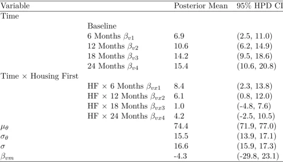
The posterior means and 95% posterior credible intervals for all model parameters from the Stan computations are presented in Table B.4. We observe that all of the posterior coefficient estimates of time effects, βev = [βv1, βv2, βv3, βv4], are positive, which confirms

the findings of Patterson et al. and in Chapter 2 (Table B.3 and Figure B.2) that, within the TAU group, we witness a dramatic upsurge in the QoL scores over time. For example, the posterior mean of βv4 is 15.0, which indicates that QoL scores rose by an average of 15

points from baseline.

An important observation is that the QoL scores tended to increase to a large extent initially and then level out. This confirms a well known result in the VAH study that all participants tended to improve dramatically after study enrollment, irrespective of whether they were allocated to HF or TAU. However, this increase occurred primarily during the early period of the study.

The important part of Table B.4 concerns the treatment by period interaction coef-ficients βvx1, βvx2, βvx3, βvx4, which are the treatment effect at each of the four follow-up

times points. For example, βvx1 was estimated as 8.4, which means that at 6 months the

QoL trajectory was on average 8.4 points higher in the HF group as compared to TAU. Furthermore, this difference was statistically significant in the sense that the 95% credible interval did not include zero.

While the time effect increases steadily from 6 months to 24 months, the treatment by period interaction, with a posterior mean of βvx1 = 8.4 at 6 months, dips at 12 and

18 months (βvx2 = 5.9, βvx3 = 0.7). A small increase is seen at 24 months (βvx4 = 4.3)

but this, along with βvx3, is deemed insignificant due to the inclusion of 0 in its 95% high

probability density (HPD) credible interval.

We conclude that although HF had a large effect on QoL scores during the first 12 months of follow-up, it nearly vanished during the second year. This finding was not reported in the linear mixed effects model of Patterson et al. [25] as it analyzed only one year of follow-up. Essentially, the improvement in outcomes for the TAU group was so substantial that it erased much of the anticipated benefit of HF. We emphasize however that the treatment

(26)

effect estimates in Table B.4 were still strictly positive at all time points, and this points to an overall conclusion of benefit albeit with larger uncertainty.

(27)

Chapter 4

Bayesian Sensitivity Analysis

(BSA) for Non-ignorable Missing

Data

4.1

Model

It was shown in the previous chapter that some of the QoL scores were missing. A natural question of interest is whether the inclusion of these missing data would distort the conclusions drawn from the analyses using only existing data, and if so, the extent of influence. The key issue is whether the data are missing at random or non-ignorable missing. However, this cannot be ascertained from observed data because we cannot tell how the missing data differs from the observed data.

To better understand the impact of non-ignorable missing data, we approach the problem from a sensitivity analysis perspective [6]. We propose a novel methodology called “Bayesian sensitivity analysis” (BSA) to explore sensitivity to nonignorable missing data. The idea is to propose a model for the complete data (observed and unobserved) that is indexed by non-identifiablesensitivity parameters that describe how the missingness is non-ignorable.

Although the data do not tell us much about the sensitivity parameters, they can still be manipulated as part of a sensitivity analysis, allowing us to examine whether the analysis results of Chapter 3 are robust to different and potentially extreme assumptions about non-ignorability. Moreover, it is straightforward to consider the sensitivity analysis within a full Bayesian analysis framework where we assign prior probability distributions to the sensitivity parameters. However, as the resulting model is not identifiable (i.e. the data

(28)

cannot distinguish between different models even asymptotically), the Bayesian method has unusual statistical properties.

We begin this chapter with proposing a modified pattern mixture model that accounts for the effect of missingness on the observations, following Hogan et al. [6].

4.1.1 Missing Data Model

LetYij be the quality of life score forithparticipant in thejthrecord, where i = 1, 2, 3,

..., 297 and j = 1, 2, 3, 4, 5 represents baseline and first to fourth visit respectively. In the ideal scenario where there is no missing data, there would be 297 _×5 = 1485 observations. LetXi be an indicator variable for the group allocation of theithparticipant, such that

Xi = 1 ifith participant is in the Housing First group = 0 ifith participant is in the Treatment as Usual group

For each participant in thejthrecord, we create a vectorfVj of length 4 to represent the

number of visit, such that

f

Vj= [0,0,0,0]for baseline (0thvisit), = [1,0,0,0]for the first visit,

= [0,1,0,0]for the second visit,

= [0,0,1,0]for the third visit,

= [0,0,0,1]for the fourth visit

Let Iij be an indicator variable for missingness in the outcome Yij, such that Iij = 1 ifYij is missing,

= 0 ifYij is observed

Note that the quantitiesIij,Xi, andfVjare always observed for all possible combinations

(29)

4.1.2 Pattern Mixture Model for Missing Data

It is clear from the study that the QoL score of each participant at a specific time is affected by the group allocation and time of visit. To model the missing data, we additionally allow QoL to depend directly on the missing indicator variable. By definition of conditional probability, we factorized the conditional distribution of Yij, Ii given Xi,fVj as

P(Yij, Iij|Xi,fVj) =P(Yij|Xi,fVj, Iij)P(Iij|Xi,fVj) (4.1)

whereP(Yij|Xi,fVj, Iij) is the pattern mixture andP(Iij|Xi,fVj) is the model for indicator

variable of missingness. The phrase “pattern mixture” is used to indicate that the marginal model for the complete data, P(Yij|Xi,fVj), is a mixture with two different components.

This differs from a selection model in that the later specifies the joint distribution ofYij and Iij through models for the marginal distribution ofYij,P(Yij|Xi,fVj), and the conditional

distribution of Iij given Yij,P(Iij|Xi,fVj, Yij) [6].

Since Yij consists of the random effect, time effect, treatment by period interaction and

bias due to missingness, it can be approximated by a Normal distribution,

Yij|Xi,fVj, Iij ∼N(θi+fVjTβev+ (fVjTβevx)Xi+ (fVjTβevm)Iij, σ2) (4.2)

where θi is the random effect with the distribution N(µθ, δθ2), βev = [βv1, βv2, βv3, βv4] is a

vector of time effects,βevx= [βvx1, βvx2, βvx3, βvx4]is a vector of treatment by period

inter-actions,σis the standard deviation, and finally the quantityβevm= [βvm1, βvm2, βvm3, βvm4]

is a vector of “bias parameters” that describe the influence of the missing indicator Iij on

the QoL score.

The quantity βevm can be interpreted as the difference in QoL score for the same

par-ticipant at each visit in the observed case and in the unobserved case, holding all other variables constant. For instance, βvm1 = 0 means that at 6 months the mean QoL scores

for missing participants is identical to that of participants with an observed QoL score (no bias, hence the data are Missing at Random). Conversely, if βvm1 = −10, QoL scores for

missing participants are on average 10 points lower than observed participants.

To further simplify the BSA method, we assumed the bias parameters are the same for all four visits, i.e.

e

βvm= [βvm, βvm, βvm, βvm].

Consequently, the user needs to specify only a single parameterβvmin order to undertake

(30)

believe that the impact of attrition on the study changed over time. However, a disadvantage is that it would require the user to specify a total of four non-identifiable bias parameters rather than just one.

Note that Equation (4.2) omits interactions between the missingness indicator Iij and

treatment. This means that we assume that, at each time point, the difference in mean QoL for observed versus unobserved participants does not depend on the assigned treatment. Thus there is a “uniform impact of missingness” that is identical in TAU versus HF. In principle the model could be extended, although with further complications of requiring more bias parameters.

To complete the pattern-mixture model specification we require a model for the missing data indicator variable, which we construct as a logistic regression model

P(Iij|Xi,fVj) =P(Iij|Xi) =δXi (4.3)

Hence in the missing data model, there are two missing data proportions: δ1 and δ0, which are the proportions of data missing when X = 1 or 0. Note that this model allows the missingness to depend on the treatment assignment (e.g. allows higher missing data in the TAU group), however it assumes that the missingness does not change over time. This assumption is a little unrealistic because the missing data are likely to be more common during later follow-up (see Table B.2). AsIij andXi are fully observed for all participants,

we can assess the adequacy of the logistic regression model.

For the sensitivity analysis, we used different values ofβvmto assess the influence of the

MNAR assumption on the estimated treatment by period interaction.

4.1.3 Parametrization of Effect of HF on QoL for the BSA Model

In the dataset, we are able to observe the conditional probability of QoL among observed participants given group allocation and visit number, P(Yij|Xi,fVj, Iij = 0) and the

prob-ability of missingness in either group, P(Iij|Xi). Therefore we can calculate the observed

treatment effect, which is E[Y|X = 1,Vf, I = 0]−E[Y|X = 0,Vf, I = 0].

However, our goal is to find out themarginal treatment effect taking into account both observed and unobserved cases, which is given byE[Y|X = 1,fV]−E[Y|X= 0,fV], where

(31)

Let δ1 = P(Iij = 1|X = 1) be the probability of missingness in the HF group, and δ0 = P(Iij = 1|X = 0) be the probability of missingness in the TAU group. Then the

expected QoL score for the TAU group is

E[Y|X = 0,fV] =E[Y|X= 0,fV, I = 1]δ0+E[Y|X= 0,fV, I = 0](1−δ0) = (µ0+fVT(βev+βevm))δ0+ (µ0+fVT(βev))(1−δ0) =µ0+fVT(βev+δ0βevm))

(4.5)

whereδ0βevm is the bias shift.

On the other hand, the expected QoL score for the Housing First group is

E[Y|X = 1,Vf] =E[Y|X= 1,Vf, I = 1]δ1+E[Y|X= 1,fV, I = 0](1−δ1) = (µ0+fVT(βev+βevx+βevm))δ1+ (µ0+fVT(βev+βevx))(1−δ1) =µ0+fVT(βev+βevx+δ1βevm))

(4.6)

whereδ1βevm is the bias shift.

Therefore the overall treatment effect can be shown to be

E[Y|X= 1,fV]−E[Y|X = 0,Vf] =fVT(βevx+ (δ1−δ0)βevm). (4.7)

This gives a simple analytical formula for exploring sensitivity to non-ignorable missing data. We see that βevx is the observed treatment effect and additionally, the quantity (δ1−δ0)βevm is the bias. If the probability of missingness is different in both groups (i.e. if δ0 ̸=δ1) and the bias parameterβevm̸= 0, there is a bias due to missingness.

4.2

Prior Distributions

(32)

Building on Chapter 3 for the Bayesian linear effects model, we assign the following prior distributions for the parameters,

µθ ∼N(0,100) σ2_θ ∼N(0,100000)+ e βv ∼N        0,        100 0 0 0 0 100 0 0 0 0 100 0 0 0 0 100               e βvx∼N        0,        100 0 0 0 0 100 0 0 0 0 100 0 0 0 0 100               σ2 ∼N(0,100000)+. (4.8)

For βvm, we used two different approaches to assign a prior distribution. First, we

assigned specific fixed values to βvm (so thatβvm is not a random variable). Seven values

ranging from -30 to 30 were selected to cover a broad range of possible values of βvm.

Thereafter, we repeated the analysis and assigned a prior βvm ∼ Uniform(−30,30). Thus

the first analysis is a classic “sensitivity analysis” in the sense that the bias parameterβvm

is fixed at a specific value that ranges over a grid in order to study the sensitivity analysis of the results, whereas the second analysis is a classic Bayesian sensitivity analysis where we model our prior beliefs about βvm as a uniform distribution.

Since the QoL scores are in the range [20, 140], it would be reasonable to assign a

N(0,100) prior to the random effect, time effect and treatment by period interaction. However, there is no information on the variances σ2_θ and σ2. As such, a diffuse prior

N(0,100000) is used.

A crucial aspect of the BSA method is justifying the range of values for βvm. Our

approach allowed βvm to vary between -30 and 30. As mentioned above the data should

reveal nothing about the true value of the βvm, even as n → ∞. Thus choosing a prior is

highly speculative and this prior will strongly influence the results. As described in section 4.1.2, βvm can be interpreted as the difference in the QoL score of the same participant

at each visit in the observed case versus the unobserved case, holding all other variables constant. Based on a review of the literature, we feel that± 30 is the maximum plausible range for βvm in the VAH data.

(33)

4.3

Computations Using Stan

In the analysis using the rstanpackage, the list of data was first defined,

int n; (number of participants)

int nobs; (number of observed records)

int nmis; (number of missing records)

int id[nobs+nmis]; (vector of participant ids of length 5n)

real yobs[nobs]; (vector of observed QoL scores of length nobs)

real x[nobs+nmis]; (vector of group allocations of length 5n)

matrix[nobs+nmis, 4] v; (matrix of visit numbers)

real betavm; (bias due to missingness) followed by list of the parameters,

real theta[n]; (random effects in linear mixed effects model)

real mu_theta; (mean of the random effects)

vector[4] betav; (time effect)

vector[4] betaxv; (time effect)

real<lower=0> sigma_theta; (sd of the random effects)

real<lower=0> sigma; (sd of the QoL)

real ymis[nmis] (missing data to be imputed) and the priors specified in the previous section.

The missing data was imputed in the following f or loop,

for (i in 1:(nmis))

ymis[i] ∼ normal(v[i+nobs] * (betav + betavm) + (v[i+nobs] * betavx) * x[i+nobs] + theta[id[i+nobs]], sigma);

with the observed data in another loop,

for (i in 1:(nobs))

yobs[i] ∼ normal(v[i] * betav + (v[i] * betavx) * x[i] + theta[id[i]], sigma);

We ran the Hamiltonian Monte Carlo algorithm for 2000 iterations with a burn-in of 1000. Sample convergence was once again assessed using the effective sample size and scale reduction factor, which are automatically generated in Stan.

(34)

4.4

Results

4.4.1 Sensitivity Analysis Where βvm is Fixed over a Specific Grid of Values

Sensitivity analysis results with fixed βvm over a specific grid of values produced

esti-mates ofβevx parameters as displayed in Table B.5. Asβvm decreases from 30 (mean QoL

for missing participants 30 points higher than observed participants) to -30 (mean QoL for missing participants 30 points lower than observed participants), we witness a clear monotonic increase in the estimates of all four treatment effect parameters βevx.

Upon closer inspection we can see that when βvm is positive (QoL for missing higher

than observed), there is no or little significant treatment effect at all four time points. Since the percentage of missingness is higher in the TAU group, higher QoL scores for missing participants would result in a smaller actual difference between HF and TAU than observed, thus overriding any perceived treatment effect.

On the contrary, negative βvm values (QoL for missing lower than observed) signify

that the actual difference in QoL between HF and TAU is larger than observed, thereby amplifying the treatment effect. Naturally, its estimates are much more significant.

The case ofβvm = 0 is trivial, as we were simply assuming that there is no difference in

QoL between missing and observed participants (i.e. MAR), which is essentially equivalent to ignoring the missing data. As such, the estimates should be very similar to those we obtained using the naïve model (Table B.4).

It should also be noted that even at an extremely low value of βvm= -30, the treatment

effect at 18 months βvx3 is still non-significant, and that at 24 months βvx4 is only slightly

significant. Whereas βvx1 stays significant throughout the range of βvm values. These

observations provide good evidence that the treatment effect is highly non-sensitive to changes in the bias parameter βvm.

4.4.2 Bayesian Sensitivity Analysis Whereβvm is a Random Variable with

Prior Distribution

We now present the BSA results, wherein we assign a prior probability distribution to

βvm. The results from Stan computations using a Uniform prior forβvmare summarized in

Table B.6. The key observation is that the posterior means and 95% HPD credible intervals of µθ, σθ2,βev,βevx and σ2 are very similar to their counterparts in the naïve model (Table

(35)

This tells us that the analysis results in the VAH dataset are robust to even quite extreme assumptions about bias from non-ignorable missing data.

Table B.4 also shows that βvm has a posterior mean of -4.3 and 95% HPD credible

interval of (-29.8, 23.1). The considerable width of this credible interval ensures that it encompasses the more extreme values ofβvm and reinforces our view thatβev,βevx are

non-sensitive to drastic changes in the bias due to missingness.

We theorize that the lack of any real difference in the BSA versus naïve analysis results can be explained by the fact that the difference in missingness between the two groups is relatively small (9.7% in HF, 21.5% in TAU, with a difference of 10.8%) and that βvm is

small in magnitude. This is to say that since only 10% to 20% of the QoL scores are missing, even extreme assumptions about MNAR data do not unduly influence the analysis results about the effect of HF on QoL.

(36)

Chapter 5

Simulations

5.1

Generating Simulated Datasets

The main comparison that is important in this thesis is Table B.4 versus Table B.6. Results in Table B.4 ignores the problem of missing data, whereas Table B.6 does a BSA that incorporates very extreme assumptions about how detrimental the missing data are. However, it is interesting to note that the results in Table B.4 and B.6 are very similar. In Table B.6 we see that the 95% HPD CIs are only somewhat wider. This is reassuring because it means that even if the missing data were very different from the observed data, it would not change the overall conclusions in the analysis of the VAH data.

We suspect that one reason that the analysis results are insensitive to missing data is that the proportion of missing QoL scores was only 9.7% in the HF group and 21.8% in the TAU group. In order to better understand the behaviour of BSA, we conducted a simulation study where we applied the BSA method to simulated data (i.e. synthetic data generated using a computer). This will better illustrate BSA in extreme situations.

In this section, we outline the procedures for generating simulated datasets using ap-propriate choices of parameters.

In the simulation, the number of participants nand number of visitsk were defined to be 300 and 5 respectively. A vector id was then created, which contained the id numbers from 1 to 300 repeated five times element-wise.

We drew the group allocation of each participant from a Binomial distribution with parameters (1, 0.5), which was stored in the vector x. This ensures that each participant

(37)

has a equal probability of being assigned to the treatment group (HF) or the control group (TAU), as is the case in the actual randomization procedure.

Corresponding to each element in the vector id, a visit number, which ranges from 0 to 4 (with 0 as the baseline) was created and stored in the vector t. This was used to construct a design matrix of dummy variables,v, where the rows represent participants at each visit and columns represent the visit number (1 to 4). An element (5x+a, y) in the matrix takes the value 1 if the(a+ 1)thentry of participant x was recorded at visit number y and 0 otherwise, with06a64.

A mean QoL score of 70 at baselinebeta.0was used, as we felt it is a realistic estimate as suggested by the VAH data.

The random effects theta.i was generated using the Normal distribution N(0, 64), with an estimated standard deviation of 8. For simplicity, we fixed the time effect beta.v

to be (10, 10, 20, 20) for each visit, with later visits resulting in a higher effect. On the other hand, the treatment by period interactionbeta.vx = (10, 10, 10, 10) would be constant throughout all four visits.

The probability of missingness in the HF and TAU group was determined to be 0.25 and 0.75 respectively in a hypothetical scenario where participants in TAU are significantly more likely to drop out of the study. Clearly, most if not all studies in real life would not see such an extreme rate of attrition on accounts of protocol restrictions,

Last but not least, we assigned a value of -5 to the bias parameter beta.vm, which we believe is a reasonable estimate of the true value in most situations.

Having determined the individual parameters, we sampled 1500 y values from the dis-tribution specified in Equation (4.2), which complete one simulated dataset. The same parameters above were used to generate 100 independent simulated datasets.

5.2

Analysis of Simulated Datasets

In order to compare the performance of estimation of the actual treatment effects, we coded both the naïve model and the BSA model, as described in Chapter 3 and 4, using the Stan language realized by the rstan package. Thereafter we applied them to the 100 simulated datasets and obtained the 95% HPD credible intervals of the treatment effect

(38)

Subsequently, we calculated the average length of the 100 credible intervals and their coverage rate of the true βvx values (10, 10, 10, 10). The coverage rate is defined as the

proportion of times that the credible intervals contain the true βvx values.

5.3

Results

Table B.7 offers clear evidence that the BSA model produces considerably wider credible intervals (average length of 23.1) of treatment effects than the naïve model (average length of 4.5). Consequently, the true values of βvx are covered approximately twice as often

by the BSA credible intervals (87%, 89%, 90%, 89%) as by the naïve credible intervals (45%, 46%, 39%, 38%). The narrow length and low coverage rate of the credible intervals produced by the naïve model substantiates the notion that it is ill-suited to handle datasets with significant amount of missingness (in this case, 50% in total), since simple omission of the missing data could result in a drastic reduction in the variance of posterior βvx and a

decisive bias in the analysis results.

The consistent performance of the BSA model in this simulated study with a large proportion of missing data suggests that it is a better choice than the existing naïve model when the bias is truly present because its credible intervals are able to cover the true values ofβvx much more frequently. This would be more apparent when the extent of missingness

(39)

Chapter 6

Discussion

In this thesis, we proposed a novel Bayesian Sensitivity Analysis method to explore sensitivity to nonignorable missing data for the outcome variable. In summary, we utilized a modified pattern mixture model for the complete data including observed and unobserved information that are indexed by non-identifiable sensitivity parameters that accounts for the effect of missingness on the observations. To use the method, the analyst must specify different values of the sensitivity parameter βevm, which can be interpreted as the average

difference in the mean QoL scores for missing versus observed participants. When each component of βevm is equal to zero, the the missingness is ignorable (MAR). Conversely,

a negative value such as -20 means that the missing individuals tend to have lower QoL scores. Alternatively, a prior probability distribution dependent on the analyst’s prior beliefs about bias should be assigned to βevm. Informative priors can be constructed from

literature reviews and expert opinions on the subject matter, while weakly informative and non-informative priors can be modelled using distributions such as Normal and Uniform. Analysis results would be presented as a table (e.g. Table B.5 and Table B.6).

The BSA method provides a major advantage over the naïve Bayesian longitudinal analysis that ignores the effect of missing data in that it produces reliable estimates of the sensitivity parameters with credible intervals as an evidence of the robustness of the other model parameters. Furthermore, in cases where there is a large difference in the frequency of missingness between the treatment and the control groups, then the credible intervals of the treatment effect parameters for BSA are markedly wider and provide much higher coverage of the true values than those for the naïve method. This is an important characteristic that enables us to ascertain the true value of treatment effect in the presence of missing data with greater confidence.

(40)

However, for the BSA model careful selection of a prior on the sensitivity parameter

e

βvm is required to conduct a meaningful analysis, as inappropriate priors would result

in confidence intervals of extreme widths of the treatment effect. Furthermore, the non-identifiability of the model dictates that the true values of its underlying parameters cannot be theoretically calculated and the data usually reveal very little about the true values of βevm. Consequently, the analyst must carefully choose the prior distribution because it

may greatly influence the analysis results. This could constitute a key challenge if there is insufficient information to determine suitable choices. For example, in the VAH dataset there no information in the literature that helps us estimate the true value ofβevm.

Curiously, non-informative priors forβevmdo not exist because the model is non-identifiable.

So for example, if we assign a prior of Unif(−1010,1010) to βevm, the resulting posterior on

the treatment effects would be infinitely wide.

Another disadvantage of the BSA is that, as are many Bayesian methods that involve Monte Carlo simulations, it could be computationally intensive, especially when a large number of missing observations exist and need to be estimated. It is also known that there is considerable computational difficulty in Bayesian MCMC simulation for non-identifiable models [30], as a result of correlated parameters in and irregular shape of the posterior distribution (Figure B.5) [26].

We applied the BSA method to the VAH data to estimate the effect of the HF interven-tion on QoL of the homeless participants. In particular, we used BSA to explore sensitivity of the analysis results to different assumptions about non-ignorable missing data (i.e. dif-ferent values of βevm). We found that there is remarkably little sensitivity to assumptions

about missing data. In other words, missingness is not a great concern as it had little effect on the analysis outcomes, which is doubtlessly good news to the researchers. Table B.5 shows that there is a slight difference in overall conclusion only when the value of βevm

approaches +30 or -30, corresponding to the extreme assumption that the QoL scores in missing participants are 30 points higher (or lower) than otherwise similar observed par-ticipants, which is not reasonable. The rather low level of sensitivity is attributable to the fact that the missingness only 10 to 15 percent.

Perhaps the most curious result of the VAH study is the diminution of the effect of Housing First in the later stages of the study, which was so apparent as to

Bayesian Sensitivity Analysis for Non-ignorable Missing Data in Longitudinal Studies