Boston University
OpenBU
http://open.bu.edu
BU Open Access Articles BU Open Access Articles
2017-08
Exploring explanations for matrix
factorization recommender
systems (Position Paper)
This work was made openly accessible by BU Faculty. Please
share
how this access benefits you.
Your story matters.
Version
Published version
Citation (published version): Bashir Rastegarpanah, Mark Crovella, Krishna Gummadi. 2017.
"Exploring Explanations for Matrix Factorization Recommender
Systems (Position Paper)." Proceedings of the FATREC Workshop on
Responsible Recommendation.
https://hdl.handle.net/2144/26683
Recommender Systems
Bashir Rastegarpanah
Boston University [email protected]Mark Crovella
Boston University [email protected]Krishna P. Gummadi
Max Planck Institute for Software Systems
gummadi@mpi- sws.org
ABSTRACT
In this paper we address the problem of finding explanations for collaborative filtering algorithms that use matrix factorization meth-ods. We look for explanations that increase the transparency of the system. To do so, we propose two measures. First, we show a model that describes the contribution of each previous rating given by a user to the generated recommendation. Second, we measure the influence of changing each previous rating of a user on the outcome of the recommender system. We show that under the assumption that there are many more users in the system than there are items, we can efficiently generate each type of explanation by using linear approximations of the recommender system’s behavior for each user, and computing partial derivatives of predicted ratings with respect to each user’s provided ratings.
ACM Reference format:
Bashir Rastegarpanah, Mark Crovella, and Krishna P. Gummadi. 2017. Posi-tion Paper: Exploring ExplanaPosi-tions for Matrix FactorizaPosi-tion Recommender Systems. InProceedings of Workshop on Responsible Recommendation at RecSys 2017, Como, Italy, August 2017 (FATREC 2017),4 pages.
https://doi.org/10.18122/B2R717
1
INTRODUCTION
Recommender systems are taking on an increasing role in shaping the impact of computing on society, and it is consequently impor-tant to develop methods for explaining the recommendations made by such systems.
Among the many possible goals for explanation [6], we focus on user-oriented explanation (explanations that assume the system is fixed) rather than developer-oriented explanation (explanations that guide system development). Within the user-oriented domain, we focus on explanations that have as their goaltransparency: provid-ing the user with an understandprovid-ing of how the system formulated a recommendation.
Among the broad class of recommender systems approaches, one can distinguishneighborhood methods,based on computing simi-larities between items or users, frommatrix factorization,which assigns items and users to a latent space in which inner product captures the affinity of a user for an item. Neighborhood methods naturally lend themselves to explanation: witness Netflix’s recom-mendations in which, for a given movie previously viewed, a set of recommended movies is proposed. In this context, the previously viewed movie is treated as an explanation.
This article may be copied, reproduced, and shared under the terms of the Creative Commons Attribution-ShareAlike license (CC BY-SA 4.0).
FATREC 2017, August 2017, Como, Italy © 2017 Copyright held by the owner/author(s). DOI: 10.18122/B2R717
Matrix factorization (MF) methods, on the other hand, can be more accurate than neighborhood methods [2], but pose a greater challenge from an explanation standpoint. The associated chal-lenges include:
• Matrix factorization methods make use of theentireset of previous recommendations – over all users and items – in formulating a single recommendation for a given user.
• Matrix factorization methods solve a non-convex optimiza-tion via heuristic methods, whose funcoptimiza-tioning can be quite opaque.
Our current work investigates two sets of corresponding ques-tions:
(1) In a context where multiple items (and users) can be said to have contributed to forming a recommendation, what is the most meaningful or useful feedback to give a user to explain a single recommendation?
(2) Given the complexity of MF approaches, are there approxi-mate representations of the behavior of MF algorithms that we can use to construct such useful feedback?
A general strategy, exemplified by [4], provides some guidance in addressing the two questions. First, explanations should be in terms that are familiar to users: broadly, they should be in terms of features rather than in terms of, e.g., latent vectors. Second, useful explanations can be in terms ofinterpretablemodels – for example, decision trees or linear models – which can be chosen as
local approximationsof a more complex nonlinear model (such as a neural network).
In the remainder of this position paper we use this general strat-egy to address the questions above. Our general approach is via the use ofgradientsof the rating function, as in recent work on classifiers (e.g., [1, 5]). First, we propose gradient based metrics ap-propriate for MF recommender systems; then we describe how, in a certain commonly encountered scenario, one may approximately compute those gradients.
2
EXPLANATIONS
Assumexijindicates the rating given by userjto itemi. To formu-late an explanation for a given recommendation, we consider the case in which the system has given userja recommendation for itemiwith an estimated rating of ˆxij. That is, the system has formed a prediction that userjwill rate itemiat ˆxijand has consequently proposed itemito the user.
In such a setting, userjmay ask:
(1) Which previous ratings have contributed the most to the predicted rating ˆxij?
FATREC 2017, August 2017, Como, Italy Bashir Rastegarpanah, Mark Crovella, and Krishna P. Gummadi
(2) Which previous ratings have the most influence over the predicted rating ˆxij? In other words, if things were different – e.g., different ratings had been provided in the past – which differences would matter most?
To answer these questions in terms familiar to users, it makes sense to use items and their ratings as the basic vocabulary (rather than, say, latent vectors). Furthermore, although an MF based rec-ommender system implicitly takes into account the set of known ratings across all users and items in making its recommendation, other users’ ratings are not under userj’s control. Hence it does not seem helpful to express our explanations in terms of ratings other than userj’s.
This leads us to propose the following kinds of explanations for MF recommender systems:
ImpactWe model each recommendation ˆxijin terms of known ratings given by the same user. That is, we formulate a model
ˆ
xij≈ X
k∈R(j)
αkxk j.
whereR(j)is the set of items that have been previously rated by userj, and we termγk =αkxk j theimpact of known ratingxk j on the predicted rating ˆxij. The model is linear to support interpretability.
Influence In order to explain the influence of the known rating
xk jon the predicted rating ˆxij, we define:
βk=∂∂xxˆij
k j
and we callβktheinfluenceofxk jon ˆxij.
We envision the use of these quantities as an interface element of the recommender system. For any given recommendation ˆxij, the interface can present the highest impact ratings (those with largestγk) and the highest influence ratings (those with largestβk), along with their values, as explanations for that recommendation.
3
ALGORITHMS
We now seek to find ways to compute approximations to impact and influence as defined in Section 2.
To start, we formalize the setting. AssumeX∈Rm×nis a par-tially observed, real-value matrix containing user ratings. Each column is associated with a user and each row is associated with an item. An MF recommender system attempts to estimate unknown elements of the rating matrix. To do so, it find factorsU∈Rℓ×m andV∈Rℓ×nsuch thatUTVagrees with the known positions in
X. The unknown ratings are then estimated by setting ˆX=UTV. More specifically, the recommender system finds factorsUand
Vby applying an algorithmAto solve the following optimization problem: U,V=arд min ˜ U,V˜ X (i,j)∈Ω (xij−u˜Ti v˜j)2 (1) whereΩindicates the set of known entries inX, ˜ui is columniof
˜
U, and ˜vjis columnjof ˜V.
3.1
U
and
V
at a local optimum
To capture the effect ofA, let us define a functionf such that for each userj,f returns the estimation of all item ratings for userj given the set of known item ratings of userj. In other words,f takes the columnxjof theobservedmatrixXas input, and returns the corresponding column ˆxjof thepredictedmatrix ˆX, i.e.,f(xj)=xˆj. Now consider the properties ofUandVat a local minimum of the objective function (1). In that case, each can be expressed as a linear function ofX. To see this, first note that for each userjwe have
f(xj)=UTvj. To capture the fact that only known entries matter in the solution of (1), we defineWjto be a binary matrix with 1s on the diagonal in positions corresponding the known entries of
xj. Then it follows thatvj is the least squares solution of
Wjxj=WjUTvj
This implies that at a local minimum of (1), the following rela-tionship holds betweenxj andf(xj):
f(xj)=UTvj =UT(UWjUT)−1
UWjxj (2)
3.2
A common case
To develop methods for approximatingγkandβk, we consider the case in which there are many more users in the system than there are items. For example, a movie recommendation system may have millions of users but only thousands of movies. In that case we formulate the following hypothesis:
Hypothesis 1. Given matrixX∈Rm×n, withn≫m, letΩbe
the set of known elements inXandAbe an algorithm that computes UandV, a local optimum of (1). Assume we change elementxijtoxij′ and rerun algorithmAto findU′andV′, thenU′is approximately equal toUand the only significant differences betweenV′andVlie in columnj.
Informal justification for Hypothesis 1 is provided in Appendix A. We find that Hypothesis 1 holds consistently in empirical studies.
3.2.1 Influence.In cases where Hypothesis 1 holds, we can proceed as follows. We start by estimating influence. Our goal is to compute the Jacobian of the functionf()evaluated atxj. That is, we seek:
J(j)= ∂f(xj)
∂xj
We callJ(j)the influence matrix of userj.
Assumeεiis a vector of sizemin which elementiisεand all the other elements are zero. In order to compute each element of the influence matrix of userj, we need to compute function
f atxj and at neighborhoods ofxj that are defined byxj +εi
fori ∈ {1, . . . ,m}. Equation (2) provides a closed form formula
of functionf()when the input is one of the user rating vectors. Moreover, under Hypothesis 1 we know that equation (2) provides an approximation forf()when the input is amodifieduser rating vector in which only one of the elements is changed. Therefore we can state that Equation (2) holds not just atxj, but also within a small neighborhood aroundxj. Then:
J(j)= ∂f∂(xj)
xj =U
T(UW jUT)−1
Interestingly, the influence matrix of each userjonly depends onUand on the set of items that have been previously rated by user
j. In particular, it does not depend on the actual ratings that user
jhas given to any previous items. So if two usersaandbhappen to have rated exactly the same set of items, although the actual rating values may differ, their influence matricesJ(a)andJ(b)will be identical.
In summary, when Hypothesis 1 holds, then for a given userj and recommended itemi, the influence of itemkisβk=J(j)
ik.
3.2.2 Impact.Next, we turn to approximating impact. In section 2 we showed that the following linear model describes the output of an MF recommender system for userjas a function of his known ratings:
f(xj)=J(j)xj
whereJ(j)is the influence matrix of userj. Therefore, the predicted rating for itemican be written as
ˆ
xij= X
(k,j)∈Ω J(ikj)xk j.
We defineγk,the impact of known ratingxk jon predicted rating ˆ
xijas
γk =Jik(j)xk j
which is simply the product of the influence of itemkon the pre-diction for itemi and the actual rating given by userj to item
k.
We emphasize that our proposed method for computingγkis only one way of quantifying impact. In other words, one may choose another linear combination of known ratings of userjthat results in ˆxijto define impact. While our method here has the interesting property that coefficients are identical to partial derivatives, one may choose another method to satisfy a different set of properties. For example, a recent work [5] studies the problem of attributing the prediction of a deep network to its input features. A similar approach can be adopted to define more elaborate measures of impact in the context of MF recommender systems.
4
EXAMPLE
To illustrate our proposal more concretely, we present an example using the MovieLens small dataset [3]. We choose the 650 most active users and the 50 most frequently rated movies. The resulting rating matrix has about 25% known entries. To this matrix we apply a well known matrix factorization algorithm (LMaFit[7]) with estimated rank 4 and obtain factorsUandV.
If Hypothesis 1 holds, then as discussed above, if usersaandb have rated the same set of items, changing the rating given by user
ato itemi(x′
ia←xia+ε) and changing the rating given by user
bto itemiby the same amount (x′
ib ←xib+ε) should have an identical effect on the predicted ratings for all other items. In other words, we have:
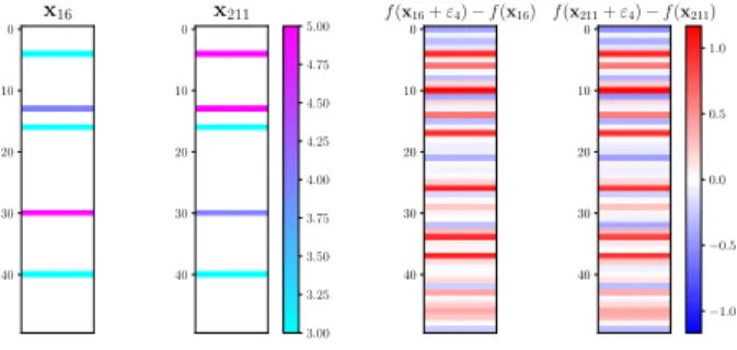
f(xa+εi)−f(xa)=f(xb+εi)−f(xb) (3) To illustrate this, we find two usersa(user 16) andb(user 211) who happen to have rated the same set of five movies in our data. Figure 1 (left side) shows the ratings given by these two users to these five movies. We then add 1 to usera’s rating for movie 4,
Table 1: Explanation forTerminator2
Rated movie Influence
Mission: Impossible (1996) 5.00
Twelve Monkeys (a.k.a. 12 Monkeys) (1995) 1.01
Star Wars: Episode IV - A New Hope (1977) -0.24
Fargo (1996) -1.65
Independence Day (1996) -2.74
rerunLMaFit, and compute the difference in predicted ratings for all movies. Next we repeat the same procedure, this time modifying only userb’s rating for movie 4. The two vectors of rating differ-ences are shown on the right side of Figure 1, and we see that the changes across all movie ratings are nearly identical.
0 10 20 30 40 x16 0 10 20 30 40 x211 3.00 3.25 3.50 3.75 4.00 4.25 4.50 4.75 5.00 0 10 20 30 40 f(x16+ε4)−f(x16) 0 10 20 30 40 f(x211+ε4)−f(x211) −1.0 −0.5 0.0 0.5 1.0
Figure 1: Users 16 and 211 have rated the same set of items. Left: original ratings; Right: changes to all predictions after modifying each user’s rating for movie 4.
To illustrate the use of influence values in practice, we show in Table 1 a simple example drawn from our dataset. The table shows for user 16, the influence of each of the 5 movies that the user has rated on the system’s predicted ratings forTerminator2. The Table shows that changing the user’s previous ratings forStar
WarsorFargowould have much less influence on the predicted rating forTerminator2than would changing previous ratings for
Mission ImpossibleorIndependence Day.
5
CONCLUSION
In this position paper we’ve proposed two kinds of explanations for increasing the transparency of matrix factorization recommender systems: influence, and impact. We argue that these allow for inter-pretable responses to questions that are important to users: “What are the most important factors yielding this recommendation?” and “What are the factors whose change would most affect this recom-mendation?” The first question provides the users an understanding of how a recommendation is generated by the system based on the actions they have made in the past, while answering the second question provides the users with information that can be used to control the system’s behavior in the future.
We have also shown that in the common case in which there are many more users than items (such as movie recommender systems), there are tractable computational approximations that can be used
FATREC 2017, August 2017, Como, Italy Bashir Rastegarpanah, Mark Crovella, and Krishna P. Gummadi
to provide numerical values for influence and impact. Interestingly, we find that in this case influence is only determined by the set of movies rated, but not by the values of the ratings given.
We expect to develop these results in both theoretical and prac-tical directions to explore the ultimate utility of these modes of explanation for matrix factorization recommender systems.
A
JUSTIFICATION OF HYPOTHESIS 1
Here we present a justification for Hypothesis 1.
We consider the case in whichn ≫m. In our analysis we make the assumption that a change toxi jonly results in changes touiandvj(i.e, we focus on the first-order approximation to the effect of AlgorithmA). Let the updated latent vectors beu′
iandv′j.
Intuitively, our argument is as follows. Updatingui tou′
i results in
changes to errors only in rowi, and updatingvjtov′
jresults in changes
to errors only in columnj. The effect of updates yieldingu′
i andv′jwill
generally attempt to decrease error at position(i,j)and will consequently tend to increase errors on other elements of rowiand columnj. Since there are many more elements in rowithan there are in columnj, an update to ui(to achieve a unit decrease in error at positioni,j) will introduce more overall error than will an update tovj. Hence the bulk of change will occur invj, whileuiwill remain relatively constant.
More formally, letei j = (xi j−uT
ivj)andL =P
i je 2
i j.Before the
change to elementxi j, the effect ofAhas been to achieve ∂u∂L
i =
∂L
∂vj =0.
These partial derivatives are:
∂L ∂ui = −2 n X k ei kvk ∂L ∂vj = −2 m X k ek juk (4)
Now, we introduce a change to the rating in position(i,j). Assuming that onlyuiandvjchange during the subsequent optimization, then applying
Aleads to: u′ k= ui+u˜ k=i uk k,i v′ k= vj+v˜ k=j vk k,j (5)
Thus our goal becomes to establish that∥v˜∥ ≫ ∥u˜∥.
Lete′be the new error values andL′be the new total squared error. At the new local optimum, we have∂L
′ ∂u′ i = ∂L′ ∂v′ j = 0. ∂L′ ∂u′ i = −2Pn ke ′ i kv ′ k = −2(e′ i jv′j+ P k,jei k′ vk) ∂L′ ∂v′ j = −2Pm k e ′ k ju ′ k = −2(e′ i ju′i+ P k,iek j′ uk) (6) Subtracting corresponding eqns in (6) and (4) and dropping factors of -2, we get: ∂L′ ∂u′ i − ∂L ∂ui = e′ i jv′j−ei jvj+ X k,j (e′ i k−ei k)vk (7) ∂L′ ∂v′ j − ∂L ∂vj = e′ i ju′i−ei jui+ X k,i (e′ k j−ek j)uk (8) Note that: e′ i k−ei k = −u˜Tvk k,j (9) e′ k j−ek j = −v˜Tu k k,i (10)
So substituting (9) and (10) into (7) and (8):
∂L′ ∂u′ i − ∂L ∂ui = e ′ i jv′j−ei jvj+ X k,j −(u˜Tv k)vk=0 (11) ∂L′ ∂v′ j − ∂L ∂vj = e′ i ju ′ i−ei jui+ X k,i −(v˜Tuk)uk=0 (12)
Now subtracting (12) from (11) we get:
e′ i j(v′j−u′i)−ei j(vj−ui)+ m X k,i (v˜Tu k)uk− n X k,j (u˜Tv k)vk=0 (13) In (13), we note that the termse′
i j(v ′ j−u
′
i)andei j(vj−ui)are small
compared to the two summation terms. Therefore we can approximately argue: m X k,i (v˜Tu k)uk ≈ n X k,j (u˜Tv k)vk (14) ˜ vT m X k,i ukuTk ≈ u˜T n X k,j vkvTk (15)
This establishes a relationship between ˜vand ˜u. To make quantitative predictions, we can assume, e.g., thatuk andvk are i.i.d. multivariate Gaussian random variablesN(0,Σ)withΣ=E[ukuT
k]=σ 2I . Then in expectation: E ˜ vT m X k,i ukuTk ≈ E ˜ uT n X k,j vkvTk (16) ˜ vT m X k,i Ef ukuTkg ≈ u˜T n X k,j Ef vkvTkg (17) (m−1)σ2v˜T ≈ (n−1)σ2u˜T (18) So we have that∥v˜∥/∥u˜∥ ≈(n−1)/(m−1).
REFERENCES
[1] David Baehrens, Timon Schroeter, Stefan Harmeling, Motoaki Kawanabe, Katja Hansen, and Klaus-Robert Müller. 2010. How to Explain Individual Classification Decisions. J. Mach. Learn. Res.11 (Aug. 2010), 1803–1831. http://dl.acm.org/ citation.cfm?id=1756006.1859912
[2] Yehuda Koren and Robert Bell. 2011.Advances in Collaborative Filtering.In Recommender Systems Handbook. Springer, 145–186.
[3] MovieLens [n. d.]. MovieLens dataset. https://grouplens.org/datasets/movielens/. ([n. d.]).
[4] Marco Tulio Ribeiro, Sameer Singh, and Carlos Guestrin. 2016. Why Should I Trust You?: Explaining the Predictions of Any Classifier. InProceedings of the 22nd ACM SIGKDD International Conference on Knowledge Discovery and Data Mining. ACM, 1135–1144.
[5] Mukund Sundararajan, Ankur Taly, and Qiqi Yan. 2017. Axiomatic Attribution for Deep Networks.CoRRabs/1703.01365 (2017). http://arxiv.org/abs/1703.01365 [6] Nava Tintarev and Judith Masthoff. 2011. Designing and evaluating explanations for recommender systems. InRecommender Systems Handbook. Springer, 479– 510.
[7] Zaiwen Wen, Wotao Yin, and Yin Zhang. 2012. Solving a low-rank factorization model for matrix completion by a nonlinear successive over-relaxation algorithm. Mathematical Programming Computation4, 4 (2012), 333–361. https://doi.org/10. 1007/s12532- 012- 0044- 1