Efficient computation of Harmonic Centrality on large networks: theory and practice

(1)

Efficient computation of Harmonic

Centrality on large networks: theory

and practice

Master Thesis

Eugenio Angriman

Monday

10

th

October, 2016

Corso di Laurea Magistrale in Ingegneria Informatica

Advisors: Prof. Geppino Pucci, Prof. Andrea Pietracaprina

Universit`a degli Studi di Padova, Scuola di Ingegneria

(2)

(3)

Abstract

Many today’s real-world applications make use of graphs to represent activities and relationships between entities in a network. An impor-tant concept in this context is the so-calledCentrality, that is a method to identify the most influential vertexes of a graph. Centrality is repre-sented through indexes such as theCloseness Centralityor theHarmonic Centrality. These indexes can be computed for each node in the net-work and they are both inversely proportional to the distance between the considered vertex and all the others. A couple of popular examples of Centrality indexes application are the recognition of the most influ-ential people inside a social network or the identification of the most cited web pages.

However, the rapid growth of the amount of available data forces us to deal with extremely large networks. Consequently, the Centrality in-dexes computation for these kind of networks is often unfeasible since it is needed to be solved the All-Pairs-Shortest-Path problem, which requires a time that is at least quadratic in the size of the network. Nev-ertheless most of the applications often necessitate to find just a small set of vertexes having the highest centrality index values or, at least, a reliable centrality indexes estimation.

In the last few years a lot of progress has been made for the effi-cient computation of the Closeness Centralityindex. D. Eppstein and J. Wang designed an approximation algorithm that efficiently estimates the value of the Closeness Centrality of each vertex of a given network while K. Okamoto, Wei C. and X proposed a fast algorithm that cal-culates the exact top-kCloseness Centralities. On the other hand, the Harmonic Centralityis a more recent metric and efficient algorithms for it have not been developed yet.

In this work we propose a Harmonic Centrality redesigned version of the efficient algorithms we cited above. We first provide the necessary theoretical background to prove the time and error bounds and then we present a Python implementation which makes use of graph-tool as main support library.

(4)

(5)

Acknowledgements

My gratitude goes to my advisors Professor Geppino Pucci and to Professor Andrea Pietracaprina for proposing me such a challenging and interesting problem. Working with them on this project allowed me not only to put a great effort into a topic I am captivated by, but also to learn a lot from it. I sincerely thank Dr. Matteo Ceccarello for his precious help and sugges-tions. For the assistance he provided to me I could rely on an excellent library and improve my code.

I am profoundly grateful to Michele Borassi and Elisabetta Bergamini for the detailed clarifications about their algorithms they provided to me. To my mother, father, brother and sister who shared their great support, thank you.

(10)

(11)

Chapter 1

Introduction

Many of today’s real-world applications make use of graphs in order to represent and analyze relationships between interconnected entities inside a

network. An important concept of network analysis is the so-called

Central-ity. Centrality is a method to measure the influence of a node on the other

nodes inside a network. In this context the influence of a node is intended as how close to all the other nodes the given node is and the distance between two nodes is represented as the length of the shortest path between them. The problem of identifying the most central nodes in a network is extremely important among a wide range of research areas such as biology, sociology and, of course, computer science.

Centrality is represented by indexes such as Closeness Centrality and

Har-monic Centrality. These indexes can be computed for each vertex in the graph that represents the network we would like to analyze. Closeness centrality was conceived by Bavelas in the early fifties when he developed the intuition that the vertexes which are more central should have lower distances to the other vertexes [2]. For each vertex in a graph, Closeness Centrality was de-fined as the inverse of the sum of the distances between the given vertex to all the other vertexes. However, for this definition to make sense the graph needs to be strongly connected because, without such condition, some dis-tances would be unlimited resulting in score equal to zero for the affected vertexes. Because of this drawback, it is more troublesome to work both with directed graphs and with graphs with infinite distances but, probably, it was not Bavela’s intention to use this metric with such graphs. Nevertheless it is still possible to apply Closeness Centrality to not strongly connected graphs just by not including unreachable vertexes into the sum of the distances. An attempt to overhaul the definition of Closeness for not strongly con-nected graphs was made in the seventies by Nan Lin [15]. His intuition

was to calculate the inverse average distance of a vertexvby weighting the

(12)

v. By definition, he imposed isolated vertexes to have centrality equals to 1. Even though Lin’s index seems to provide a reasonable solution to the problems related with the Bavela’s definition of Closeness, it was ignored in the following literature.

Later in 2000 the idea underneath the concept of Harmonic Centrality was introduced by Marchiori and Latora who were facing the problem of pro-viding an effective notion of ”average shortest path” for the vertexes of a generic network. In their work [16] they proposed to replace the average

distance, that was used for the Closeness centrality, with theharmonic mean

of all distances. If we assume that 1/∞=0 this kind of metric has the advan-tageous property to handle cleanly infinite distances we typically encounter in unconnected graphs. In fact the average of finite distances can be mislead-ing, especially in large networks where a large number of pairs of nodes are not reachable. In this cases the average distance may be relatively low just because the graph is almost completely disconnected [3].

The formal definition of theHarmonic Centralitywas introduced by Yannick

Rochat in a talk at ASNA 2009 (Application of Social Network Analysis). He took inspiration from the work of Newman and Butts who gave a brief definition of this centrality metric as the sum of the inverted distances a few years before [20], [5]. The definition given by Yannick also includes a nor-malization term equals to the inverse of the number of vertexes minus one in order to obtain centrality index between zero and one that is cleaner and more preferable [25].

A couple of years later Raj Kumar Pan and Jari Saram¨aki adopted a very

similar approach in their article on temporal networks [23] in order to deal

with Temporal Closeness Centrality. Concisely, they used the same definition of Harmonic Centrality given by Yannick to compute the Temporal Close-ness Centrality. The only difference is that Pan and Saram¨aki considered an

”average temporal distance”τij between two vertexesi,j∈ Vinstead of the

shortest distancedij. As they wrote in their paper this metric allowed them

”to better account for disconnected pairs of nodes”.

In the last decades the amount of available data rose exponentially and the Centrality computation has became as important as computationally unfea-sible. In the 2000s researchers proposed some new and faster approaches to compute the Closeness Centrality on large networks or a reasonable approx-imation of it.

To begin with, in 2004 David Eppstein and Joseph Wang designed a random-ized approximation algorithm for the computation of Closeness Centrality in weighted graphs. Their method can estimate the centrality of all vertexes

with high probability within a(1+ε)factor inO(logn/ε2(nlogn+m))time.

This is possible by selecting a subsetSofΘ(logn/ε2)random vertexes, then

they estimate the centrality of each node using only the vertexes inSas the

(13)

However, the majority of the applications require to calculate the top-k most central vertexes of a graph. For this purpose Kazuya Okamoto, Wei Chen and Xiang-Yang Li presented in 2008 a new algorithm that ranks

the exact top-k vertexes with the highest Closeness Centrality in O((k+

n2/3log1/3n)(nlogn+m)). Their strategy makes use of the Eppstein et al.

algorithm in order to obtain an estimation of the centrality of each vertex.

Then, they create a candidate setHwith the top-k+kˆ most central vertexes

of the estimated vertexes. Finally, they compute the exact Closeness

Central-ity for each element inside H[21].

Another algorithm for the fast computation of the exact top-kCloseness

Cen-tralities was published in 2015 by Michele Borassi, Pierluigi Crescenzi and Andrea Marino. They designed a BFSCut function that is called for each

vertex v in the graph. Briefly, this function starts the Breadth First Search

using v as source and it stops as soon as an upper bound of the Closeness

Centrality ofv is less than thek-th Closeness Centrality [4].

So far efficient algorithms for the approximation or the exact computation of the Harmonic Centrality have not been designed yet, probably for the reason that it is a more recent metric than the Closeness Centrality. Actually the algorithm presented by Borassi et al. has already been generalized by the same authors in order to compute also the Harmonic Centrality. The purpose of our work is to provide high performance algorithms for both the computation and approximation of the Harmonic Centrality on large networks. Therefore, we re-designed the approaches described by Eppstein et al. and Okamoto et al. in order to obtain for the Harmonic Centrality the same results they achieved with the Closeness Centrality. Then, we will compare these two approaches with both the basic algorithm and the with the algorithm designed by Borassi et al. Furthermore, since neither Eppstein et al. nor Okamoto et al. specified the exact number of random samples to choose for their algorithms (they provided provided an asymptotic term only), we will change the multiplicative constants in front of the asymptotic terms in order to verify whether is it possible to reduce the running time of the algorithms without compromising their precision.

The main results we achieved through this work are the following. First of all we created a strong theoretical background that supports the efficient computation of the Harmonic Centrality index. More precisely we proved the following two statements:

• It is possible to approximate all the Harmonic centralities of a graph

within a ε error bound for each vertex in O

_log_n

ε2 (nlogn+m)

time through the Eppstein et al. algorithm we redesigned

• It is possible to compute the exact top-k Harmonic centralities of a

graph with high probability inOk+n23 log

1 3 _n

(14)

through our new implementation of the Okamoto et al. algorithm Furthermore, we observed that not only both the algorithms we implemented are considerably faster than the standard approach that solves the APSP problem which is quite obvious, but our new version the Eppstein et al. ap-proximation algorithm is, in some cases, even more competitive than the

Borassi et al. implementation, especially for bigger networks and higher k

values.

Another interesting aspect of our experimental results concerns the preci-sion achieved by our approximation algorithm. In short we noticed that the actual errors were considerably lower than the corresponding upper bound

ε and if we lower the number of random samples the error grows linearly.

This means that it is possible to save a considerable amount of time by reduc-ing the number of random samples without compromisreduc-ing the algorithm’s precision.

We applied these conclusions also on our revised version of the Okamoto

et al. algorithm and we noticed that it could still compute the exact top-k

Harmonic centralities but with a considerable reduction of its running time. Our algorithms have been entirely implemented in Python 3.5.2 [1] and we used the library graph-tool 2.18 [24] for network support since it can be easily integrated into Python scripts but all its algorithms are written in C++ for better performances.

This thesis is organized as follows. In Chapter 2 we formally introduce the required background including notations, definitions and the terminology that will be used in the following chapters.

Chapter 3 is dedicated to a thorough description of the Eppstein et al., Okamoto et al. and Borassi et al. algorithms for the computation of the Closeness Centrality.

Chapter 4 is concerned with the description of how we adapted these algo-rithm for the computation of the Harmonic Centrality including a complete theoretical support.

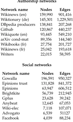
Chapter 5 presents and comments the experimental setup and the results in terms of time and precision we obtained by executing our algorithms on several large social and authorship networks.

Finally, Chapter 6 summarizes the conclusions of this work and illustrates some indications for potential future developments.

(15)

Chapter 2

Preliminaries

In the previous chapter we mentioned the importance of the centrality con-cept in the large network analysis context and we illustrated two main cen-trality indexes which are largely used in a wide range of today’s applications. We also briefly summarized three efficient strategies for both the approxima-tion and the fast computaapproxima-tion of the Closeness Centrality index.

Before describing in detail these techniques, let us give some fundamental definitions.

2.1

Centrality definitions

Let G = (V,E) be a strongly connected graph with n = |V| and m = |E|.

TheCloseness Centralityindex is defined as follows [22]:

Definition 2.1 Given a strongly connected graph G = (V,E), the Closeness Cen-trality of a vertex v ∈V is defined as:

c(v) = |V| −1

∑w∈Vd(v,w)

(2.1) where d(v,w)denotes the geodesic (i.e. shortest) distance from vertex v to w.

Another way to expressc(v)is the following [4]:

c(v) = |V| −1

f(v) , f(v) =_w

∑

_∈_Vd(v,w) (2.2)

where f(v)is also known as thefarnessofv.

However, if G is not strongly connected the definition becomes more

(16)

we imposed(v,w) =∞for each pair of unreachable vertexes, thenc(v) =0

for eachvthat cannot reach all the vertexes in the graph, which is not very

useful. The most common generalization that can be found in the literature is the following:

Definition 2.2 Given a graph G = (V,E), the closeness centrality of a vertex v∈V is defined as:

c(v) = (|R(v)| −1) 2

(|V| −1)∑_w_∈_R₍_v₎d(v,w) (2.3)

where R(v) is the set of vertexes that are reachable from v.

On the other hand theHarmonic Centralityindex is defined as follows:

Definition 2.3 Given a graph G = (V,E), the Harmonic Centrality of a vertex v∈V is defined as:

h(v) = 1

|V| −1_w_∈_V

∑

_,_w₆₌_v 1

d(v,w) (2.4)

where d(v,w) represents the geodesic distance between v and w.

In the literature the normalization term is often omitted, consequently the Harmonic Centrality is also defined as:

h(v) =

∑

w∈V,w6=v

1

d(v,w) (2.5)

Hereafter we will refer to the harmonic centrality according to the Definition 2.3 because it always takes values between 0 and 1 which can be compared more easily.

2.2

Description and complexity of the problem

Nearly all today’s applications that exploit the concept of centrality are

in-terested in identify thek ≥1 most central nodes in a network i.e. the top-k

centralities. Formally, the problem is defined as follows:

Definition 2.4 (Top-kCentrality Problem) Given a graph G= (V,E), a top-k centrality problem is to find:

argmax_V˜⊆V,|V˜|≥k min v∈_V˜ c(v), V˜ (2.6) where c(v) is an arbitrary centrality index.

(17)

2.2. Description and complexity of the problem

Note that the set ˜V might be greater than k for the reason that different

vertexes may have the same centrality value, so they should be included. The easiest and most naive strategy to solve this problem is to compute the

centrality of each vertex in the graph, sort them and return thekmost central

vertexes. This is equivalent to solve the All-Pairs Shortest-Path problem (APSP) that is known to be unfeasible for large networks. Several algorithms

can solve the APSP problem in O nm+n2logn

time [9, 12] and others in

O n3

time [8] or even up toO n2_log_n

for random graphs [6, 10, 17, 19]. However, all of them are too slow, specialized, or excessively complicated and, for this reason, faster algorithms for the computation or approximation of the centrality indexes are needed.

(18)

(19)

Chapter 3

Efficient algorithms for the

computation of Closeness Centrality

In the previous chapters we illustrated the importance of the top-k

central-ity problem and the difficulties of solving it efficiently because it is almost equivalent to the All-Pairs Shortest-Path problem. Since it is unfeasible to solve the APSP problem for large networks, researchers designed fast and reliable algorithms for both the approximation and the exact computation

of the top-kCloseness Centralities of a network. In this chapter we illustrate

in detail three of these algorithms and the theory underneath them.

3.1

Fast Top-k Closeness Centrality computation

We now present the algorithm designed by M. Borassi, P. Crescenzi and A.

Marino for the efficient computation of the exact top-kCloseness centralities

of a graph. The core of their intuition is represented by the BFSCut function they call for each vertex in the graph. This function calculates an upper

bound ˜c(v) of the Closeness Centrality of the current vertex v ∈ V and it

stops as soon as ˜c(v) is less than the current k-th Closeness centrality c_k.

Otherwise, it completes the BFS from node v and stores its Closeness

Cen-trality valuec(v). It is important to point out that, in a worst case scenario,

the complexity of this algorithm is the same as the the naive approach of

solving SSSP for each all vertexes in the graph that isO(n2logn+nm). The

authors nonetheless noticed that the BFSCut function is far more efficient than solving APSP for the vast majority of the real-world cases.

Their algorithm’s running time is also boosted by a degree-descending sort of all the graph’s vertexes in order to run the BFSCut function for the highest degree vertexes first. This is thought to minimize the probability of

perform-ing a full BFS for non-top-k most central vertexes.

(20)

intro-duce and demonstrate the correctness of the elements we will use such as the Closeness upper bound and other functions.

3.1.1 Upper bound of the Closeness Centrality

The BFSCut function takes as input two main parameters: the current node

v∈Vand the currentk-th Closeness centralityck. Then, it updates the value

of ˜c(v)whenever the exploration of thed-th level of the BFS starting fromv

is finished (d ≥1). ˜c(v)is then obtained from a lower bound on the farness

ofv:

Lemma 3.1 (Farness lower bound)

f(v)≥ f˜d(v,r(v)):= fd(v)−γ˜d+1(v) + (d+2)(r(v)−nd(v))

where:

• r(v)is the number of reachable vertexes from v

• fd(v)is the farness of node v up to distance d, that is:

f_d(v) =

∑

w∈Nd(v)

d(v,w)

where Nd(v)is the set of vertexes at distance at most d from v i.e.:

N_d(v) ={w∈V :d(v,w)≤ d}

• γd+1is the number of vertexes at distance exactly d+1from v.

• γ˜d+1is an upper bound onγd+1 and it is defined as follows:

˜

γd+1 =

∑

w∈Γd(v)

outdeg(u)≥γd+1(v) =|Γd+1(v)|

whereΓ_d+1(v)represents the set of vertexes at distance exactly d+1from v.

• n_d+1(v)is the number of vertexes at distance at most d+1from v i.e.:

nd+1(v) =|Nd+1(v)|=|{w∈V: d(v,w)≤ d+1}|

Proof Clearly, for eachd≥1 it holds that:

f(v)≥ fd(v) + (d+1)γd+1(v) + (d+2)(r(v)−nd+1(v))

(21)

3.1. Fast Top-kCloseness Centrality computation

f(v)≥ fd(v) + (d+1)γd+1(v) + (d+2)(r(v)−γd+1−nd(v))

= fd(v)−γd+1(v) + (d+2)(r(v)−nd(v))

Finally, since ˜γd+1 =∑u∈Γd(v)outdeg(v)≥γd+1(v)we have:

f(v)≥ fd(v)−γ˜d+1+ (d+2)(r(v)−nd(v))

At this point the upper bound of the Closeness Centrality of v can be

ex-pressed as: ˜ c(v) = (r(v)−1) 2 (n−1)f˜d(v) ≥c(v) (3.1)

and, apart from r(v), all quantities are available as soon as all vertexes in

Nd(v)are visited by a BFS.

3.1.2 Computation of r(v)

The computation ofr(v)depends on the properties of the input graphG=

(V,E). More precisely, if G isstrongly connected then r(v) = n while, if G

is undirected but not necessarily connected, r(v) can be calculated in linear

time. More effort is required if Gis directed and not strongly connected.

Directed and not Strongly Connected Graphs

For this particular situation we assume to know for r(v) an upper bound

α(v)>1 and a lower boundω(v). We will useα(v)andω(v)to calculate a

lower bound on 1/c(v): Lemma 3.2 1 c(v) ≥λd(v):= (n−1)min ˜ f_d(v,α(v)) (α(v)−1)2, ˜ f_d(v,ω(v)) (ω(v)−1)2

Proof From Lemma 3.1 it follows that:

f(v)≥ fd(v)−γ˜d+1(v) + (d+2)(r(v)−nd(v))

If we denotea =d+2:

f(v)≥ f_d(v)−γ˜_d+1(v) +a(r(v)−nd(v))

(22)

Finally, if we denoteb= γ˜d+1(v) +a(nd(v)−1)− fd(v):

f(v)≥a(r(v)−1)−b

where a > 0 (because d > 0), b > 0 (because ˜γ_d+1(v) ≥ 0) and nd(v) ≥ 1

(because v∈ Nd(v)). Therefore:

fd(v) =

∑

w∈Nd(v)

d(v,w)≤d(nd(v)−1)< a(nd(v)−1)

the first inequality holds because if w = v then d(v,w) = 0, otherwise

w∈Nd(v)⇒1≤d(v,w)≤d. The second inequality is trivial.

Considering the generalized definition of Closeness Centrality given by Equa-tion 2.2 it follows that:

1 c(v) = (n−1) f(v) ((r(v)−1)2 ≥(n−1) a(r(v)−1)−b (r(v)−1)2

Let us denote x = r(v)−1 and consider the function g(x) = ax_x−2b in order

to study its minima. Its first order derivative g0(x) = −ax_x+3 2b is positive for

0<x< 2_ab and negative forx> 2_ab if we consider only the positive values of

x (which is reasonable if we assumer(v)>1). This means that 2_ab is a local

maximum and there are no local minima forx > 0. Consequently, for each

closed interval[x1,x2]wherex1adx2are positive, the minimum ofg(x)for

x>0 is reached in x1or x2. Since 0< α(v)−1≤r(v)−1≤ ω(v)−1:

g(r(v)−1)≥min(g(α(v)−1),g(ω(v)−1))

Computingα(v)and ω(v) The computation ofα(v)andω(v)can be done

during the pre-processing phase of the algorithm. Let G = (V,E) be the

weighted acyclic graph made by the strongly connected components (SSCs)

corresponding to the graphG= (V,E). It is defined as follows:

• V is the set of SSCs of G.

• for any C,D∈ V, (C,D) ∈ E if and only if∃ v ∈ C, u ∈ Ds.t. (v,u) ∈

E.

• for each SSC C ∈ V the weight w(C) = |C|, that is the number of

(23)

So, if vertexesvanduare in the same SSCC, then:

r(v) =r(u) =

∑

D∈R(C)

w(D) (3.2)

where R(C)represents the set of SSCs that are reachable fromC inG. This

means that we only need to compute a lower bound α(C) and an upper

bound ω(C) once for every SSC C in G. To do so we first compute a

topo-logical sort {C1,· · · ,Cl}ofV (where ifCi,Cj ∈ E, theni<j) such that:

• Cl is asinknode i.e. outdeg(Cl) =0.

• All sink nodes are placed consecutively at the end of the SSCs list.

then we use a dynamic programming approach in reverse topological order

starting fromCl: α(C) =w(C) + max (C,D)∈Eα(D) ω(C) =w(C) +

∑

(C,D)∈E ω(D) (3.3)

Note that processing the SSCs in reverse topological order (fromCl down to

C1) ensures us that the values on the right hand side of the equation above

are available when computing the valuesα(C)andω(C).

For example, at the first iteration we must compute α(Cl) and ω(Cl). We

know that outdeg(C_l) = 0 so α(C) = ω(C) = w(C_l) = |C_l|. This applies

to every other sink node in the list and provides the needed information to

computeα(Ci)andω(Ci)for the remaining non-sink nodes.

3.1.3 The algorithm

Here we illustrate the algorithm’s pseudo-code including the BFSCut func-tion for each combinafunc-tion of directed, undirected, strongly and not strongly connected plus the dynamic programming algorithm for the computation of the SSCs in the graph.

(24)

Algorithm 1TopK Clos(G= (V,E),k)

1: Preprocessing(G)

2: x_k ←0

3: foreach nodev∈V do

4: c(v)←0

5: end for

6: forv∈ Vin decreasing order of degreedo

7: c(v)←BFSCut(v,xk) 8: ifc(v)6=0then 9: xk ←Kth(c) 10: end if 11: end for 12: returnTopK(c) Where:

• xk is thek-th greatest closeness computed until now

• Kth(c)is a function that returns thek-th biggest element ofc

• TopK(c)is a function that returns thekbiggest elements ofc

The Preprocessingphase of the algorithm takes linear time and can be used

(25)

Algorithm 2BFSCut(v,xk)function in the case of strongly connected graphs

1: Create queue Q 2: Q.enqueue(v) 3: Markv as visited 4: d ←0; f ←0; ˜γ←0;nd←0; 5: while!Q.isEmptydo 6: u←Q.dequeue()

7: if d(v,u) > d then //all nodes at level d−1 have been visited, ˜c

must be updated 8: f˜← f −γ˜+ (d+2)(n−nd) 9: c˜← n−_˜1 f 10: ifc˜≤xk then 11: return0 12: end if 13: end if 14: f ← f+d(u,v) 15: γ˜ ←γ˜+ outdeg(u) 16: nd←nd+1

17: forw in adjacency list of udo

18: ifw.visited == f alsethen

19: Q.enqueue(w) 20: w.visited←true 21: end if 22: end for 23: end while 24: return n−_f1

(26)

Algorithm 3 BFSCut(v,xk) function in the case of undirected graphs (not necessarily connected) 1: Create queue Q 2: Q.enqueue(v) 3: Mark vas visited 4: d←0; f ←0; ˜γ←0; nd←0; 5: while!Q.isEmptydo 6: u←Q.dequeue() 7: ifd(v,u)>dthen

8: r←BFSCount(u)//Returns the number of reachable nodes from

u 9: f˜← f−γ˜ + (d+2)(r−nd) 10: c˜← n−1 ˜ f 11: ifc˜≤xk then 12: return0 13: end if 14: end if 15: f ← f +d(u,v) 16: γ˜ ←γ˜+outdeg(u) 17: nd←nd+1

(27)

Algorithm 4BFSCut(v,x_k)function in the case of directed and not strongly connected graphs 1: Create queue Q 2: Q.enqueue(v) 3: Markv as visited 4: d ←0; f ←0; ˜γ←0;nd←0; 5: while!Q.isEmptydo 6: u←Q.dequeue() 7: ifd(v,u)>dthen

8: (α,ω) ← GetBounds(u) //αand ω have been computed for all

SSCs in the Preprocessing 9: fα ← fd(u)−γ˜ + (d+2)(α−nd) 10: fω ← fd(u)−γ˜+ (d+2)(ω−nd) 11: λd←(n−1)min fα (α(v)−1)2, fω (ω(v)−1)2 12: ifλd >0then 13: c˜← 1 λd 14: ifc˜≤ x_k then 15: return0 16: end if 17: end if 18: end if 19: f ← f+d(u,v) 20: γ˜ ←γ˜+ outdeg(u) 21: nd←nd+1

(28)

Algorithm 5 Dynamic programming algorithm to compute for each SSC

in G the lower bound α(C) and the upper bound ω(C) to the number of

reachable verticesr(v) 1: (V,E)←graph of SSCs 2: V0 ←topological sort ofV 3: l← |V | 4: A←~0 //|A|=l 5: Ω←~0 //|Ω|=l 6: fori=l−1 down to 0do 7: ifV0[i].outdeg==0then 8: A[i] =V[i].weight 9: Ω[i] =V[i].weight 10: else 11: O← {w∈ V s.t. (V[i],w)∈ E } 12: A[i]← V[i].weight+maxj∈OA[j] 13: Ω[i]← V[i].weight+∑_j_∈_OΩ[j] 14: end if 15: end for 16: fori=l−1 down to 0do 17: forv∈ V[i]do 18: α(v) = A[i] 19: ω(v) =Ω[i] 20: end for 21: end for 22: return(A,Ω)

(29)

3.2. Fast Closeness Centrality Approximation

3.2

Fast Closeness Centrality Approximation

In this section we describe the Closeness Centrality approximation algo-rithm conceived by D. Eppstein and J. Wang for undirected and weighted

graphs. They were inspired by a particular feature called small world

phe-nomenon that has been empirically observed to be typical of many social

networks [18, 28]. This kind of networks are characterized by O(logn)

di-ameters instead of O(n). The strategy we are going to illustrate provides a

near-linear time(1+ε)-approximation to the Closeness Centrality of all the

nodes of a network of this type.

Shortly, the main intuition is the following: instead of solving the APSP problem they compute the Single-Source Shortest-Paths (SSSP) from each

node contained in a subset S of random samples to all the other vertexes

(S⊂V). This technique allows them to estimate the centrality of eachv∈V

to within an additive error ofε∆inO logn/ε2(nlogn+m)time with high

probability, where ε>0 is the upper error bound for a single vertex

central-ity and ∆ is the diameter of the graph. The approximated vertex centrality

is calculate using the average distance to the sampled vertexes.

3.2.1 The algorithm

As we can see from the pseudo-code of Algorithm 6 (RAND), this

approxi-mation algorithm takes as inputs a graph G and the number of samples k.

Then, it performs two main actions: it selects uniformly at random k

sam-ples from V and it solves the SSSP problem with each of them as source.

Finally it computes an inverse Closeness Centrality estimator 1/ ˆc(v)of the

inverse Closeness Centrality 1/c(v)for eachv∈V.

Algorithm 6RAND(G = (V,E), k) D. Eppstein - J. Wang Closeness Cen-trality approximation algorithm.

1: fori=1 tokdo

2: vi ←pick a vertex uniformly at random fromV

3: Solve SSSP problem withvi as source

4: end for

5: foreachvinVdo

6: c(v)←cˆ(v)

7: end for

Let us point out thatkis not arbitrary but it has been defined by the authors

as Θ logn/ε2. The estimated value of the closeness centrality used for

(30)

ˆ c(v) = 1 ∑k i=1 nd(vi,v) k(n−1) (3.4) ˆ

c(v) estimates of 1/c(v) as the inverse of the average distance to the

sam-pled vertexes, which is normalized by the _k₍_nn₋₁₎ term.

In conclusion, if we adopt the O(nlogn+m) algorithm designed by

Fred-man and Tarjan for solving the SSSP problem [9], the total running time

of this approximation algorithm is O(km) for unweighted graphs and

O(k(nlogn+m)) for weighted graphs. Thus, given that k = Θ logn/ε2,

we obtain an O mlogn/ε2 algorithm for unweighted graphs and an

O logn/ε2(nlogn+m)algorithm for weighted graphs.

3.2.2 Theoretical analysis

So far we described how the algorithm operates, which conditions the in-put graph must satisfy and how many samples we should choose. Now we must demonstrate that the algorithm RAND computes the inverse Closeness

Centrality estimator ˆc(v)for eachv ∈ V to within an upper error bound of

ξ = ε∆ with high probability. For this purpose we will refer to the errors

on the estimated Closeness centralities as independent, bounded and identi-cally distributed random variables in order to exploit the Hoeffding lemma on probability bounds for sums of independent random variables, that is:

Lemma 3.3 (Hoeffding [11]) If x1,x2, . . . ,xk are independent random variables,

ai ≤xi ≤bi andµ=E

h

∑k i=1xki

i

is the expected mean, than forξ >0:

Pr ( ∑k i=ixi k −µ ≥ξ ) ≤2e− 2k2ξ2 ∑k i=1(bi−ai)2 (3.5)

In other words, we will denotexi as _c_ˆ(1vi)−

1

c(vi), 1≤i≤k.

For the reason that Hoeffding’s lemma requires the empirical mean of the

x1,x2, . . . ,xnrandom variables i.e. ∑ki=1 xki to be equal toµ, we need to prove

that Eh_c_ˆ₍1_v₎i= _c₍1_v₎.

Theorem 3.4 Given that:

c(v) = n−1 ∑n i=id(vi,v) and cˆ(v) = 1 ∑k i=1 nd(vi,v) k(n−1) then,Eh_c_ˆ₍1_v₎i= _c₍1_v₎.

(31)

3.2. Fast Closeness Centrality Approximation

Proof It is trivial that:

E 1 ˆ c(v) =E " k

∑

i=i nd(vi,v) k(n−1) # = = n k(n−1)E " k

∑

i=1 d(vi,v) #

Since we can interpret the geodesic distance between d(vi,v) as a random

variable and, given X1,X2, . . . ,Xkrandom variables, it is known that E

∑k i=1Xi = ∑k i=1E(Xi). It follows that: n k(n−1)E " k

∑

i=1 d(vi,v) # = n k(n−1) k

∑

i=1 E[d(vi,v)]

The expected value of the geodesic distance between vi and v can be

ex-pressed as: E[d(vi,v)] = 1_n∑nj=1d(vj,v). So we have that:

n k(n−1) k

∑

i=1 E[d(vi,v)] = n k(n−1) k

∑

i=1 1 n n

∑

j=1 d(vj,v) = 1 k(n−1) n

∑

j=1 k

∑

i=1 d(vj,v) = 1 k(n−1) n

∑

j=1 kd(vj,v) = 1 n−1 n

∑

j=1 d(vj,v) = 1 c(v) So far we have proven that we are operating under the hypothesis required by the Hoeffding’s bound. Now we can use it to demonstrate the following theorem:

Theorem 3.5 Given an undirected, connected and weighted graph G = (V,E), with high probability the algorithm RAND computes the inverse of the Closeness Centrality estimator cˆ(v) for each vertex v ∈ V to within an upper error bound

ξ =ε∆usingΘ

_log_n

ε2

(32)

Proof As we suggested before we can exploit the Hoeffding’s bound to

cal-culate an upper bound on the probability that the error of ˆc(v) is greater

thanξ =ε∆. This can be done by imposing:

x_i = nd(vi,v) n−1 , µ= 1 c(v), ai =0, bi = n∆ n−1

Thus, given that E[1/ ˆc(v)] =1/c(v)we can re-write Equation 3.5 as follows:

Pr 1 ˆ c(v)− 1 c(v) ≥ξ =Pr ( k

∑

i=1 nd(vi,v) k(n−1) − 1 c(v) ≥ ξ ) =Pr ( k

∑

i=1 xi k −µ ≥ξ ) ≤2e− 2k2ξ2 ∑k i=1(bi−ai)2 ≤2e − 2k2ξ2 k(_nn₋∆₁)2 =2e−Ω kξ2 ∆2

In order to meet the required bounds we impose ξ = ε∆ and k = αlog_ε2n,

whereα≥1. It follows that:

2e−Ω kξ2 ∆2 = e−Ω αε 2_∆_{2 log}_n ε2∆2 = e−Ω(αlogn) = e−Ω(lognα) ≤1/nα

This implies that the probability of the error to be greater than ξ at any

vertex in the graphGis upper-bounded by 1/nα_{. This gives a 1/}_nα−1_≤_1/_n

probability of having errors greater thanε∆in the whole graph.

3.3

Exact top-k Closeness centralities fast computation

The last algorithm we are going to present in this chapter was introduced by K. Okamoto, W. Chen and X. Li for the exact computation of the

(33)

3.3. Exact top-kCloseness centralities fast computation graphs. The main strategy is based on the combination of the

approxima-tion algorithm we described in the previous secapproxima-tion with the exact algo-rithm. More precisely, this algorithm executes the RAND algorithm with

l = Θ(k+n2/3log1/3n) samples first in order to find a candidate set E of

top-k0 vertexes, where k0 > k. To guarantee that all final top-k vertexes fall

inside the E set the authors suggest to carefully choose k0 using the bound

given in the proof of Theorem 3.5. Once the Eset has been found the exact

algorithm is used to compute the average distances for each v ∈ E and,

fi-nally, the actual top-k greatest Closeness centralities can be extracted.

Briefly, under certain conditions, the algorithm we illustrate in this section

ranks all the top-k vertexes with greatest Closeness Centrality in O((k+

n2/3_log1/3_n₎₍_n_log_n₊_m₎₎_{time with high probability.}

3.3.1 The algorithm

Algorithm 7 (TOPRANK) takes as input an undirected, connected and weighted

graph G = (V,E), the number of top ranking vertexes it should extract

(k) and the number of samples (l) to be used by the approximation

algo-rithm RAND. First of all, TOPRANK uses the RAND algoalgo-rithm with a set

S, |S| = l of random sampled vertexes to estimate the average distance ˆav

for each v ∈ V. Next, it names all the vertexes in the graph to ˆv1, ˆv2, . . . , ˆvn

such that ˆav1 ≤ aˆv2 ≤ · · · ≤ aˆvn, where ˆavi = 1/ ˆcvi, and creates the E set

(|E|=k0) of top-k0 vertexes with greatest estimated Closeness Centrality. As

final step, TOPRANK computes the exact average shortest-path distances of

all vertexes inEand returns the top-k Closeness centralities.

Algorithm 7TOPRANK(G = (V,E),k,l) K. Okamoto, W. Chen, X. Li exact

top-kCloseness centralities algorithm.

1: Use algorithm RAND with a setSoflsampled vertexes to obtain the

es-timated average distance ˆav ∀v∈V. Rename all vertexes to ˆv1, ˆv2, . . . , ˆvn

such that ˆavˆ1 ≤aˆvˆ2 ≤ · · · ≤aˆvˆn

2: Find ˆv_k

3: ∆ˆ ← 2 minu∈Smaxv∈Vd(u,v) //d(u,v)has been computed for all u ∈

S,v∈Vat step 1 and ˆ∆is determined inO(ln)time

4: Compute candidate set E as the set of vertexes whose estimated average

distances are less than or equal ˆavˆk+2f(l)∆ˆ

5: Calculate exact average shortest-path distances of all vertexes inE

6: Sort the exact average distances and return the top-k highest closeness

centralities

Note that the candidate set E is computed at line 4 of Algorithm 7 as ”the

set of vertexes whose estimated average distances are less than or equal to ˆ

(34)

f(l) =α

r

logn

l (3.6)

whereα> 1. The authors made this choice in order to define a 1/2n2 upper

bound to the probability of the estimation error at any vertex in the graph

of being at least f(l)∆. This is based on setting ε = f(l) in the proof of

Theorem 3.5, the details are illustrated in the following theoretical analysis section (3.3.2).

In this section we formally demonstrate that, under the assumptions we made on the sampling techniques and on the input graph, the TOPRANK

algorithm computes exactly the top-k Closeness centralities with high

prob-ability inO((k+n2/3log1/3n)(nlogn+m))time.

First and foremost we must prove that if we choose f(l)as in Equation 3.6

than with low probability the approximation error at any vertex in the graph

will be greater than f(l)∆:

Theorem 3.6 If the f(l) function is chosen as in Equation 3.6 then the error of the estimation of c(v)for each v ∈ V is greater than f(l)∆with less than 1/2n2 probability.

Proof The proof is based on settingε= f(l)in the Hoeffding’s bound used

in Theorem 3.5: Pr 1 ˆ c(v)− 1 c(v) ≥ξ ≤2e − 2l2ξ2 k(_nn₋∆₁)2 = 2 e2lξ2(n_n−_∆1)2 (As before we setξ =ε∆) = 2 eloglognn2lε2(n−n1) 2 = 2 n2l ε 2 logn(n −1 n ) 2 Now we setε= f(l) =α r logn l ! = 1 n2lβ_llog_logn_n Whereβ=α2 = 1 n2β ≤ 1 n2

(35)

3.3. Exact top-kCloseness centralities fast computation Note that in the fifth line of the proof we included both the numerator (2)

and the multiplicative constant n−_n12inside the constant β≥1.

Now we have the enough elements to prove the correctness of the TOPRANK algorithm:

Theorem 3.7 Given an undirected, connected and weighted graph G = (V,E), if the distribution of the average distances is uniform with range c∆, where c is a constant and ∆ is the diameter of G, the TOPRANK algorithm ranks the top-k vertexes with the greatest Closeness Centrality inO((k+n2/3_log1/3_n₎₍_n

logn+

m))with high probability when we choose l =Θ(n2/3log1/3n).

We will proceed by demonstrating two main lemmas: Lemma 3.8 supports the correctness of the algorithm’s output while Lemma 3.9 defines the time required by the algorithm. The strategy adopted by the authors is to prove the correctness of the TOPRANK regardless its time performances first. Then they proved that, if a particular condition is met, the same result can also be achieved in the required time limits. The results achieved by these two lemmas can be summarized in Theorem 3.7.

Lemma 3.8 Algorithm TOPRANK ranks all the top-k vertexes with the highest Closeness Centrality correctly with high probability with any parameter l configu-ration.

Proof Given that the TOPRANK algorithm computes the exact average

dis-tances for each v ∈ E we must show that, with high probability, the set E

(line 4 of Algorithm 7) contains all the top-k vertexes with the lowest exact

average distance.

Let T = {v1,v2, . . . ,vk} be the set of the exact top-k Closeness centralities

and ˆT = {vˆ1, ˆv2, . . . , ˆvk} be the set of the estimated top-k Closeness

central-ities returned by the RAND algorithm. Since the errors in the estimation

of the average distances ˆav are independent and in Theorem 3.6 we proved

for any vertexvthat the estimated average distance ˆav is greater than f(l)∆

with probability less than 1/2n2 i.e.:

Pr(¬ {av− f(l)∆≤aˆv ≤av+ f(l)∆})≤ 1

2n2

it follows that, for each v∈V:

Pr ¬ ( ^ v∈T ˆ av≤ av+ f(l)∆≤ avk+ f(l)∆ )! ≤ k

∑

i=1 Pr(¬ {avi− f(l)∆≤aˆvi ≤avi + f(l)∆})≤ k 2n2 (3.7)

(36)

This means that, with probability at least 1−k/2n , there exist at least k

vertexes in T whose estimated average distance ˆav is less than or equal to

avk+ f(l)∆. Similarly: Pr  ¬    ^ ˆ v∈_Tˆ avˆ≤ aˆvˆ+ f(l)∆≤ aˆvˆk+ f(l)∆     ≤ k

∑

i=1 Pr(¬ {avî − f(l)∆≤ aˆvî ≤avî+ f(l)∆})≤ k 2n2 (3.8)

which means that there exist at least k vertexes ˆv ∈ Tˆ whose real average

distanceavˆ is less than or equal to ˆavˆk+ f(l)∆with probability greater than

1−k/2n2_{. Thus:}

Pr(¬ {avk ≤aˆvˆk+ f(l)∆})≤

k

2n2 (3.9)

At this point from the 3.7 inequality we know that for each v ∈ T, ˆav ≤

avk+ f(l)∆. By combining this result with the 3.9 inequality it follows that:

Pr  ¬    ^ ˆ v∈_Tˆ ˆ av ≤avk+ f(l)∆≤aˆvˆk+2f(l)∆      ≤ k n2 (3.10)

Since at line 4 the TOPRANK algorithm includes in setE each vertex such

that ˆavˆ ≤ aˆvˆk+2f(l)∆ˆ as the final part of this proof we have to prove that

∆≤∆ˆ.

For anyw∈ Vwe have that:

∆= max v,v0_∈_Vd(v,v 0₎_≤ _max v,v0_∈_V d(w,v) +d(w,v 0₎ = max v,v0_∈_Vd(w,v) +_vmax_,_v0_∈_Vd(w,v 0₎ =2 max v∈V d(w,v) and thus: ∆≤2 min w∈S max v∈V d(w,v) =∆ˆ

Therefore for each v ∈ T, ˆav ≤ aˆvˆk+2f(l)∆ˆ with probability at least 1−

(37)

3.4. Conclusions

in Eall the top-kvertexes with lowest average distance and it computes the

exact top-kCloseness centralities with high probability.

Lemma 3.9 If the distribution of the estimated average distances is uniform with range c∆, where c is a constant number and∆is the diameter of the input graph G, then TOPRANK takesO((k+n2/3log1/3n)(nlogn+m))time when we choose l=Θ(n2/3log1/3n).

Proof At line 1 the TOPRANK algorithm executes the RAND algorithm

us-ing lsamples which takesO(l(nlogn+m))time as we saw in the previous

section. Since the distribution of the estimated average distances is uniform

with rangec∆, there are 2n f(l)∆ˆ/c∆ vertexes between ˆavˆk and ˆavˆk+2f(l)∆ˆ.

Since 2n f(l)∆ˆ/c∆ ∈ O(n f(l)), the number of vertexes inE isk+O(n f(l))

and therefore TOPRANK takes O((k+O(n f(l)))(nlogn+m))time at line

5. In order to lower the total running time at lines 1 and 5 as much as

possible, we should select lthat minimizesl+n f(l)that is:

∂ ∂l(l +n f(l)) =0 ∂ ∂l l +nα r logn l ! =0 1− nα 2 p logn l3/2 =0

this leads to:

l=n·α 2 2₃ ·log13 _n₌Θ n23 ·_log13 _n

In conclusion, if we choose l = Θ(n2/3log1/3n) the TOPRANK algorithm

takesO(n2/3_log1/3_n₍_log_n₊_m₎₎_{time at line 1 and it takes}_O₍₍_k₊_n2/3_log1/3_n₎_·

(nlogn+m))time at line 5. Consequently, since all the other operations are

asymptotically cheaper, TOPRANK takesO((k+n2/3log1/3n)(nlogn+m))

total running time.

3.4

Conclusions

In this chapter we illustrated three fast approaches for the approximation and the exact computation of the Closeness Centrality of a graph with high probability, we demonstrated their correctness and we calculated their asymptotic running time. In Chapter 4 we will provide a detailed descrip-tion of how these algorithms can be applied to the Harmonic Centrality.

(38)

(39)

Chapter 4

Efficient Algorithms for the Harmonic

Centrality

In the previous chapter we exposed in detail three efficient algorithms for both the computation and the approximation of the Closeness Centrality. In this chapter we introduce three new algorithms for the computation of the Harmonic Centrality inspired by the BFSCut function, RAND and TOPRANK.

4.1

Borassi et al.

strategy applied to the Harmonic

Centrality

In this section we describe how the BFSCut function could be applied for the

computation of the exact top-kHarmonic centralities. The main challenge is

represented by finding and proving an upper bound forh(v).

4.1.1 An upper bound for h(v)

As Borassi et al. did in their work we would like to define an upper bound ˜

h(v) to the Harmonic Centrality of node v in order to stop the BFS from

that node if ˜h(v)is less than thekth greatest Harmonic Centrality computed

until now. Of course, ˆh(v) has to be updated whenever all the vertexes of

thedth level of the BFS tree have been visited, d≥1.

Lemma 4.1 h(v)≤h˜d(v,r(v)):= hd(v) + ˜ γd+1 (d+1)(d+2)+ r(v)−nd(v) d+2 (4.1)

where hd(v)is the Harmonic Centrality of node v up to distance d.

(40)

h(v)≤ h_d(v) + γd+1(v) d+1 + r(v)−n_d+1(v) d+2 Sincend+1(v) =γd+1(v) +nd(v), h(v)≤hd(v) + γd+1(v) d+1 + r(v)−γd+1(v)−nd(v) d+2

Finally, since ˜γd+1 =∑u∈Γd(v)outdeg(v)≥γd+1(v)

h(v)≤ hd(v) + ˜ γd+1(v) (d+1)(d+2)+ r(v)−nd(v) d+2 We can exploit this property to efficiently compute the top-k Harmonic cen-tralities using Algorithm 1 and a slightly revised version of the BFSCut func-tion reported in Algorithm 2 for strongly connected graphs which were de-scribed in Section 3.1.3.

Finally, for directed and not (strongly) connected graphs we know that the

Harmonic Centrality h(v) depends only on the reachable vertexes from v

since the others give no contribution. In this case r(v) is hard to compute

but, with the purpose to find an upper bound toh(v), we can try to find an

upper bound tor(v)sinceh(v)is directly proportional tor(v).

Borassi et. al. already provided an upper bound ω(v) tor(v)so we could

re-use part of Algorithm 5 of Section 3.1.3 to computeω(v)for each vertex.

(41)

4.1. Borassi et al. strategy applied to the Harmonic Centrality

Algorithm 8Revised BFSCut(v,hk)function for the computation ofh(v) in

the case of strongly connected graphs

1: Create queue Q 2: Q.enqueue(v) 3: Markv as visited 4: d ←0; h←0; ˜γ←0;nd←0; 5: while!Q.isEmptydo 6: u←Q.dequeue()

7: if d(v,u) > d then //all nodes at level d−1 have been visited, ˜h

must be updated 8: h˜ ←h+ γ˜ (d+1)(d+2)+ n −nd d+2 9: if _n₋h˜₁ ≤ xk then 10: return0 11: end if 12: d←d+1 13: end if 14: ifu6=vthen 15: h←h+_d₍_u1 ,v) 16: end if 17: γ˜ ←γ˜+ outdeg(u) 18: nd←nd+1

19: forwin adjacency list ofudo

21: Q.enqueue(w) 22: w.visited←true 23: end if 24: end for 25: end while 26: return _n₋h₁

(42)

Algorithm 9Revised BFSCut(v,xk)function in the case of undirected graphs

(not necessarily connected)

1: Create queue Q 2: Q.enqueue(v) 3: Mark vas visited 4: d←0;h←0; ˜γ←0;nd←0; 5: while!Q.isEmptydo 6: u←Q.dequeue() 7: ifd(v,u)>dthen

8: r←BFSCount(u)//Returns the number of reachable nodes from

u 9: h˜ ←h+ γ˜ (d+1)(d+2)+ r−nd d+2 10: if _n₋h˜₁ ≤ x_k then 11: return0 12: end if 13: d←d+1 14: end if 15: ifu6=v then 16: h←h+ 1 d(u,v) 17: end if 18: γ˜ ←γ˜+outdeg(u) 19: nd←nd+1

20: forwin adjacency list ofu do

(43)

4.1. Borassi et al. strategy applied to the Harmonic Centrality

Algorithm 10BFSCut(v,xk)function in the case of directed and not strongly

connected graphs 1: Create queue Q 2: Q.enqueue(v) 3: Markv as visited 4: d ←0; h←0; ˜γ←0;nd←0; 5: while!Q.isEmptydo 6: u←Q.dequeue() 7: ifd(v,u)>dthen

8: ω ← GetBound(u) //ω has been computed for all SSCs in the

Preprocessing 9: h˜ ←h+ γ˜ (d+1)(d+2)+ ω −nd d+2 10: ifh≤ xk then 11: return0 12: end if 13: end if 14: ifu6=vthen 15: h←h+_d₍_u1_,_v₎ 16: end if 17: γ˜ ←γ˜+ outdeg(u) 18: nd←nd+1

(44)

4.2

Fast Harmonic Centrality Approximation

The D. Eppstein and J. Wang strategy we presented in Section 3.2 can be adapted to the Harmonic Centrality with little effort. The steps of the al-gorithm are almost the same as RAND but it is necessary to provide the

Harmonic Centrality’s correct estimation of vertex v i.e. ˆh(v). In

conclu-sion we obtained an algorithm that computes with high probability a ε

-approximation of the Harmonic Centrality (ε > 0) of an undirected,

con-nected and weighted graph that takesO(logn/ε2(nlogn+m)time.

4.2.1 The algorithm

Similarly to the RAND algorithm, RAND H takes as inputs a graphGand

the number of samples k. Then it extracts k random samples from V and

solves the SSSP problem for each extracted sample as source. Finally it

computes an Harmonic Centrality estimator ˆh(v)for each v∈V.

Algorithm 11RAND H(G = (V,E),k) Our redesigned version of the RAND algorithm for the computation of the Harmonic Centrality.

1: fori=1 tokdo

2: vi ←pick a vertex uniformly at random fromV

3: Solve SSSP problem withvi as source

4: end for

5: foreachvinV do

6: h(v)←hˆ(v)

7: end for

As in the previous chapter we want the number of random samples to be

k = Θ(logn/ε2). Thus, we define the Harmonic Centrality estimator as

follows: ˜ h(v) = n k(n−1) k

∑

i=1 1 d(v_i,v) (4.2)

Similarly to Equation 3.4 we are expressing the Harmonic Centrality esti-mator as the normalized average of the inverse distances to the sampled

vertices, withn/kas normalization term.

Our purpose is now to demonstrate that the RAND H algorithm we sketched

in the previous section provides aε-approximation of the Harmonic

Central-ity of each v ∈ V to withinO(logn/ε2(nlogn+m) time with high

(45)

4.2. Fast Harmonic Centrality Approximation

with the approximation error|hˆ(v)−h(v)| as random variable, we start by

demonstrating that the expected value of ˆh(v)is equal toh(v)as requested

by Lemma 3.3.

Theorem 4.2 Given that:

h(v) = 1 |V| −1_w_∈_V

∑

_,_w₆₌_v 1 d(v,w) and h˜(v) = n k(n−1) k

∑

i=1 1 d(vi,v) then,E h ˆ h(v)i= h(v). Proof Ehhˆ(v)i=E " n k(n−1) k

∑

i=1 1 d(vi,v) # = n k(n−1)E " k

∑

i=1 1 d(vi,v) #

Again we can interpret 1/d(v_i,v)as a random variable and so E

h ∑k i=1 d(v1i,v) i = ∑k i=1E h 1 d(vi,v) i

and it follows that:

= n k(n−1) k

∑

i=1 E 1 d(vi,v) Since Eh_d₍_v1 i,v) i = 1_n_∑n_j₌₁ 1 d(vj,v) (we impose 1 d(vj,v) = 0 if vj = v) we have that: = n k(n−1) k

∑

i=1 1 n n

∑

j=1 1 d(vj,v) = 1 k(n−1) n

∑

j=1 k

∑

i=1 1 d(vj,v) = 1 k(n−1) n

∑

j=1 k d(vj,v) = 1 n−1 n

∑

j=1 1 d(vj,v) =h(v)

(46)

Theorem 4.2 allows us to use the Hoeffding’s bound to prove the high prob-ability bound for the RAND H algorithm.

Theorem 4.3 Given an undirected, connected and weighted graph G = (V,E), algorithm RAND H computes the estimatorhˆ(v)of the Harmonic Centrality h(v)

to within aε>0error for all vertexes v ∈V usingΘ(logn/ε2)samples with high

probability.

Proof We apply the Hoeffding’s bound with the following assumptions:

xi = n n−1 1 d(vi,v) , µ= h(v), ai =0 andbi = n n−1. It follows that: Prn hˆ(v)−h(v) ≥ε o =Pr ( k

∑

i=1 n k(n−1) 1 d(v_i,v)−h(v) ≥ε ) =Pr ( k

∑

i=1 xi k −µ ≥ε ) ≤2e− 2k2ε2 ∑k i=1(bi−ai)2 ≤2e− 2k2ε2 k(_n₋n₁)2 =2e−Ω(kε2) Usingk =αlogn

ε2 samples withα≥1 leads to:

2e−Ω(kε2)₌ _e−Ω αlogn ε2 ε 2 = 1 eΩ(lognα₎ ≤ 1 nα

This means that at any vertex v ∈ V the estimation error |hˆ(v)−h(v)| is

greater thanεwith probability less than 1/nαand 1/n1−αin the whole graph.

In other words all the vertexes in the graph are affected by an error which

is less thanεwith probability at least 1−1/n.

Finally, since the time-expensive operations executed by algorithm RAND H

are equivalent to the operations of algorithm RAND (solving l times the

(47)

4.3. Fast top-k Harmonic centralities exact computation

time of O(logn/ε2(nlogn+m)) and returns the correct output with high

probability.

4.3

Fast top-k Harmonic centralities exact computation

The last algorithm we worked on is the by K. Okamoto, W. Chen and X. Li exact approach we exposed in Section 3.3. Our purpose was to modify the

TOPRANK algorithm in order to efficiently compute the exact top-k

Har-monic centralities with high probability. As the authors did, we exploited the approximation algorithm RAND H we introduced in the previous

sec-tion in order to create a candidate set H, |H| = k0 > k. Then, we adopted

the exact approach to compute the exact Harmonic centralities for allv∈ H.

In the end we obtained a O((k+n2/3log1/3n)(nlogn+m))algorithm that

calculates the exact top-KHarmonic centralities of an undirected, connected

and weighted graph with high probability.

4.3.1 The algorithm

Similarly to TOPRANK, the TOPRANK H algorithm takes as input an

undi-rected, connected and weighted graph G = (V,E), the number of top

rank-ing vertexes k and how many samples the RAND H algorithm should use

to calculate the Harmonic Centrality estimators ˜h(v). Then, as we can see

from Algorithm 12 pseudo-code, all vertexes in V are named according to

their approximated Harmonic Centrality value i.e. ˆv1, ˆv2, . . . , ˆv2 such that:

ˆ

hvˆ1 ≤ hˆvˆ2 ≤ · · · ≤ hˆvˆn. Next, the candidate set H is created as the set of

vertexes whose estimated Harmonic centrality is greater than or equal to ˆ

hvˆk−2f(l). More formally:

H= nvi ∈ V: ˆhvˆi ≥hˆvˆk−2f(l)

o

(4.3)

where f(l)is defined as in Equation 3.6

We now need to demonstrate the correctness of the TOPRANK H algorithm and its time requirements.

(48)

Algorithm 12 TOPRANK H(G = (V,E), k, l) Our redesigned version of

the TOPRANK algorithm for the computation of the top-k exact Harmonic

centralities.

1: Use algorithm RAND H with a set S of l sampled vertices to obtain

the estimated harmonic centrality ˆhv ∀v ∈ V. Rename all vertices to

ˆ

v1, ˆv2, . . . , ˆvnsuch that ˆhvˆ1 ≤ hˆvˆ2 ≤ · · · ≤hˆvˆn

2: Find ˆhk

3: Compute candidate set H as the set of vertices whose estimated

har-monic centralities are greater than or equal to ˆhvˆk−2f(l)

4: Calculate exact harmonic centralities for all vertices in H

5: Sort the exact harmonic centralities and return the top-k

As in the previous chapter we start by proving that the RAND H algorithm

will give us an ε-approximation of the Harmonic Centrality of each vertex

v∈Vwith high probability. Then we will use this result to demonstrate the

time performances of TOPRANK H and the correctness of its output.

Theorem 4.4 If the f(l)function is chosen as in Equation 3.6 then, ifε>0:

∀v∈V, |hˆ(v)−h(v)|<ε

with high probability.

Proof The strategy is to use the Hoeffding’s bound settingε= f(l)i.e.:

Prn hˆ(v)−h(v) ≥ ε o ≤2e−2l2ε2/l( n n−1)2 = 2 e2lε2(n−_n1)2 = 2 e2log n lognlε2(n −1 n ) 2 = 2 n2 lε 2 logn(n −1 n ) 2 We now setε=α 0 r logn l ! = 1 n2β llogn llogn Where β= α02 ≥1 = 1 n2β ≤ 1 n2

(49)

4.3. Fast top-k Harmonic centralities exact computation Note that in the fifth line we included both the numerator 2 and the factor

(n−_n1)2_{inside the constant} _β_≥_1.

At this point we are ready to demonstrate the correctness of the TOPRANK H algorithm using the result we achieved with Theorem 4.4. Basically we have to prove the following theorem:

Theorem 4.5 Given an undirected, connected and weighted graph G = (V,E), if the distribution the of the estimated Harmonic centralities among the vertexes in V is uniform in range cU, where c > 0 andU= [0, 1], with high probability the

TOPRANK Halgorithm ranks the top-k vertexes with the greatest Harmonic

Cen-trality in O((k+n2/3log1/3n)(nlogn+m))if we choose l = Θ(n2/3log1/3n)

samples.

We can prove this theorem by separating it into two lemmas: Lemma 4.6 and 4.7.

Lemma 4.6 The TOPRANK H algorithm ranks all the top-k vertexes with the greatest Harmonic Centrality correctly with high probability and with any parame-ter l configuration.

Proof We need to prove that with high probability the candidate set H

cre-ated at the 3rd line of the TOPRANK H algorithm contains all the top-k

vertexes with the greatest Harmonic Centrality.

Let T = {v1,v2, . . . ,vk}be the set of the exact top-k Harmonic centralities

and ˆT = {vˆ1, ˆv2, . . . , ˆvk}be the set of the top-k estimated Harmonic

central-ities returned by the RAND H algorithm. Since in Lemma 4.4 we

demon-strated that |hˆ(v)−h(v)| ≥ ε for each v ∈ V with probability less than

1/2n2_:

Pr¬nhv− f(l)≤hˆv ≤hv+ f(l)

o

≤ 1

2n2

it follows that, for each v∈V:

Pr ¬ ( ^ v∈T ˆ hv ≥hv− f(l)≥hvk− f(l) )! ≤ k

∑

i=1 Pr¬nhvi − f(l)≤hˆvi ≤hvi+ f(l) o ≤ k 2n2

This inequality means that, with probability at least 1−k/2n2_{, there are at}

least k vertexes in H whose estimated Harmonic Centrality is greater than

(50)

Pr  ¬    ^ ˆ v∈_Tˆ hvˆ ≥hˆvˆ− f(l)≥hˆvˆk− f(l)     ≤ k

∑

i=1 Pr¬nhvî − f(l)≤hˆvî ≤hvî+ f(l) o ≤ k 2n2

which shows that, with probability at least 1−k/2n2, there are at least k

vertexes in ˆH whose exact Harmonic Centrality is greater than ˆhvˆk − f(l).

Moreover, this implies that hvk ≥ hˆvˆk− f(l) with high probability. If we

combine this result with the first inequality we obtain that:

Pr ¬ ( ^ v∈T hvˆ ≥hvk− f(l)≥hˆvˆk−2f(l) )! ≤ k n2

Therefore, for eachv∈ H, ˆhv≤ aˆvˆk−2f(l)with probability at least 1−1/n

(since k ≤ n). In conclusion, we proved that the TOPRANK H algorithm

includes all the top-k vertexes with greatest Harmonic Centrality in the

can-didate setHwith high probability.

Now we can evaluate the complexity of the TOPRANK H algorithm which will have a smaller additive constant than TOPRANK since it does not need

to approximate the graph diameter ˆ∆.

Lemma 4.7 If the distribution of the estimated Harmonic centralities among the vertexes in V is uniform in range cU, where c > 0 and U = [0, 1], with high probabilityTOPRANK Hranks the top-k vertexes with the greatest Harmonic Cen-trality inO((k+n2/3_log1/3_n₎₍_n_log_n₊_m₎₎_{if we choose l}₌ _Θ₍_n2/3_log1/3_n₎

samples.

Proof We know from Chapter 3 that solving the SSSP problem takesO(nlogn+

m) time. Therefore TOPRANK H takes O(l(nlogn+m)) time at its first

step.

Since the distribution of the estimated Harmonic centralities is uniform in

rangecU then there are 2n f(l)/cvertexes between ˆhvˆk−2f(l)and, obviously,

2n f(l)/c∈ O(n f(l)). Thus, the number of vertexes in H isk+O(n f(l))and

this implies that TOPRANK H takesO((k+O(n f(l)))(nlogn+m))time at

line 4.

Finally, as the authors did in Lemma 3.9, we choose l in order to

mini-mize the total running time at line 4 that is l = Θ(n2/3log1/3n).

There-fore, under the assumptions we made, the TOPRANK H algorithm takes

(51)

4.4. Conclusions

4.4

Conclusions

In this chapter we presented a redesigned version of the algorithms we ex-posed in Chapter 3. Our aim was to obtain new strategies to approximate and calculate efficiently the Harmonic Centrality of the vertexes of a graph. Up there, we achieved our objective from a theoretical point of view. In the next chapter we will report and comment the experimental results achieved by the implementation of our algorithms. We will examine their perfor-mances in terms of time and precision and provide a comparison between them and both the naive algorithm and Borassis et al. .

(52)

(53)

Chapter 5

Experimental Results

This chapter is dedicated to the experiments we performed on several bench-mark networks. We measured the performances in terms of time and pre-cision of our Python implementation of the algorithms we exposed in the previous chapter.

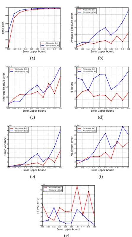
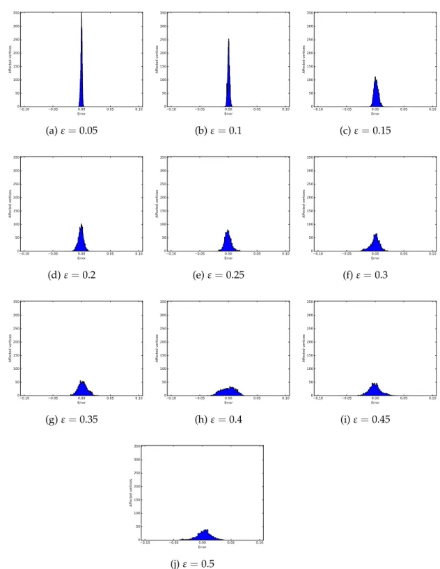
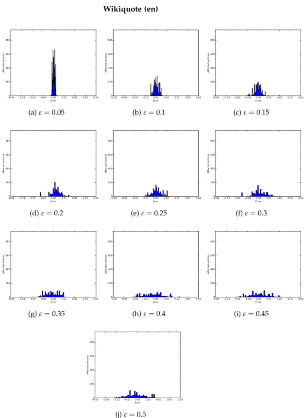
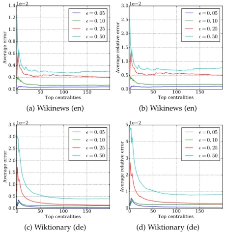
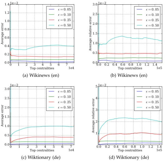
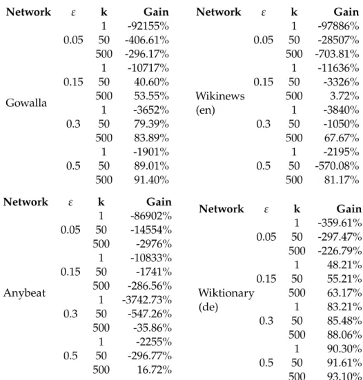
Our purpose was firstly to verify the correctness of our theoretical results into a practical scenario. Therefore we compared the running time of our randomized algorithms with the time requested by both solving APSP and the Borassi’s et al. algorithm. Then we analyzed the errors made by the ap-proximated algorithm RAND H in terms of average absolute error, average relative error and error variance. For what concerns the TOPRANK H

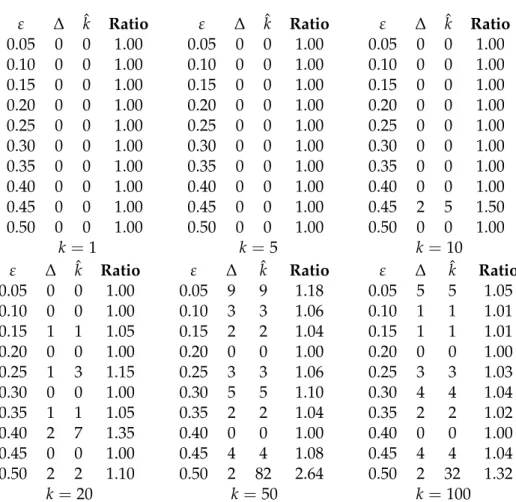
algo-rithm we checked whether the top-kgreatest Harmonic centralities it found

were correct or not.

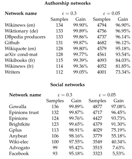
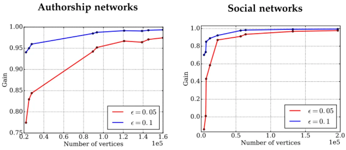
Since the RAND H algorithm achieved excellent results in terms of precision

(the error was far below the high probability boundε) we performed several

additional experiments in order to see whether it was possible to boost the algorithm’s time performances by halving the number of random samples

without violating the error bound ε. We noticed that, with such

configu-ration, the RAND H precision was not compromised. Thus we proceeded by applying the same modification also in the TOPRANK H algorithm and, finally, halving again the number of random samples of the RAND H algo-rithm.

We observed that, despite the lower number of samples, the precision of the TOPRANK H algorithm was slightly affected but it could be adjusted with a