Growth and Poverty Reduction in

(1)

The Trade-Off Among Carbon Emissions, Economic

India

VIJAY PRAKASH OJHA

Rajiv Gandhi Institute for Contemporary Studies (RGICS) New Delhi, India

SANDEE Working Paper No. 12-05 August 2005

South Asian Network for Development and Environmental Economics (SANDEE) PO Box 8975, EPC 1056

(2)

Published by the South Asian Network for Development and Environmental Economics (SANDEE), PO Box 8975, EPC 1056 Kathmandu, Nepal.

Telephone: 977-1-552 8761, 552 6391 Fax: 977-1-553 6786

SANDEE research reports are the output of research projects supported by the South Asian Network for Development and Environmental Economics. The reports have been peer reviewed and edited. A summary of the findings of SANDEE reports are also available as SANDEE Policy Briefs.

National Library of Nepal Catalogue Service: Vijay Prakash Ojha

The Trade-off Among Carbon Emission, Economic Growth and Poverty Reduction in India (SANDEE Working Papers, ISSN 1813-1891; 2005 - WP 12)

ISBN: 99946-810-1-X Key Words 1. CGE model 2. Carbon Emissions 3. Economic Growth 4. Poverty Reduction 5. India 6. Climate Change 7. Carbon Tax policy

8. Tradable Emission Permits

The views expressed in this publication are those of the author and do not necessarily represent those of the South Asian Network for Development and Environmental Economics or its sponsors unless otherwise stated.

(3)

The South Asian Network for Development and Environmental

Economics

The South Asian Network for Development and Environmental Economics (SANDEE) is a regional network that brings together analysts from different countries in South Asia to address environment-development problems. SANDEEs activities include research support, training, and information dissemination. SANDEE is supported by contributions from international donors and its members. Please see

www.sandeeonline.org for further information about SANDEE.

SANDEE is financially supported by International Development Research Centre (IDRC), The Ford Foundation, Mac Arthur Foundation , Swedish International Development Cooperation Agency (SIDA) and Norwegian Agency for Development Cooperation (NORAD).

Technical Editor

Priya Shyamsundar

English Editor

Carmen Wickramagae

Comments should be sent to Vijay Prakash Ojha, Rajiv Gandhi Institute for Contem-porary Studies (RGICS) New Delhi, India. Email: vpojha@gmail.com

(4)

(5)

LIST OF TABLES

Table 1 : Energy consumption in India (petajoules) 2 Table 2 : Energy consumption and carbon emission trends 3

Table 3 : The policy simulations 17

Table 4 : BAU Scenario and the policy simulations: Selected 30 variables in 1990

Table 5 : BAU Scenario and the policy simulations: Selected 30 variables in 2020

Table 6 : Macro variables and carbon emissions of the BAU scenario 31

Table 7 : Energy Use 31

Table 8 : Carbon tax rates 31

Table 9 : Energy Prices (percentage difference from BAU scenario) 32 Table 10 : Carbon emissions (percentage share of fossil fuels) 32

Table 11 : Carbon emissions 32

Table 12 : Per capita carbon emissions 33

Table 13 : GDP 33

Table 14 : Consumption 33

Table 15 : Poverty ratio (in percent) 34

Table 16 : Number of poor 35

LIST OF FIGURES

Figure 1 : The production structure 8

Figure 2 : BAU Scenario: Growth rates of macro variables 35

(7)

Abstract

This study examines the consequences of a) a domestic carbon tax policy, and, b) participation in a global tradable emission permits regime on carbon emissions, Gross Domestic Product (GDP), and poverty, in India. The results, based a computable general equilibrium model of the Indian economy, show that a carbon tax policy that simply recycles carbon tax revenues to households imposes heavy costs in terms of lower economic growth and higher poverty. However, the fall in GDP and rise in poverty can be minimized or even prevented if the emission restriction target is a very mild one and tax revenues are transferred to the poor. A soft emission reduction target is all that India needs to set for itself, given that even a ten percent annual reduction in aggregate emissions will bring down its per capita emissions to a level far below global per capita emissions. On the other hand, participation in the tradable emission permits regime opens up an opportunity for India to sell surplus permits. India would then be able to use the revenues from permits to speed up GDP growth and poverty reduction and keep its per capita emission below the 1990 per capita global emissions level.

Key words: CGE model, carbon emissions, economic growth, poverty reduction, India, climate change, carbon tax policy, tradable emission permits.

(8)

(9)

The Trade-Off Among Carbon Emissions, Economic Growth and Poverty Reduction in India

Vijay Prakash Ojha 1. Introduction

The linkage between carbon emission reduction, economic growth and poverty alleviation is an issue of immense relevance for India. India is highly vulnerable to global warming and global climate change caused by emissions of greenhouse gases such as carbon dioxide. The adverse effects of climate change would in all likelihood retard the developmental process and aggravate poverty. At the same time, Indias per capita carbon emission is already very low. It is 0.26 tonne per annum, which is one-fourth of the world average per capita emission of one tonne per annum (Parikh et al, 1991). In other words, Indias per capita contribution to global warming problem is a relatively minor one. However, because of its large and growing population, its total emissions are large. Internationally, India is expected to stabilize its energy related carbon emissions1_{. Moreover, the fact that India has a real stake in a global policy}

regime to stabilize global carbon emissions is being realized in Indian policy circles. More specifically, Indian policy makers are beginning to see the need to understand the implications for India of a Kyoto-type global emissions trading regime.

At the domestic level, India is concerned with the reduction of carbon emissions whether a global system of tradable emission permits materializes or not. This concern, however, is a very long term one. Switching over to non-polluting sources of energy such as, hydro and nuclear, is often mentioned as a strategy that will sweep away the problem of carbon emissions. A medium term policy option such as a carbon tax, however, is viewed with suspicion, largely because of its likely adverse impact on economic growth and poverty reduction. For a low-income country like India, the more pressing need obviously is achieving poverty reduction rather than controlling carbon emissions. Nevertheless, it would be worthwhile exploring how much, if at all, carbon taxes trade-off growth and poverty reduction, and what compensatory mechanisms can be built into the system to mitigate the undesirable effects of carbon taxes on GDP growth and poverty alleviation.

This study seeks to answer three questions related to policy trade-offs between carbon emission reduction, growth and poverty: a) what are the economic and distributional impacts of imposing carbon taxes when tax revenues are recycled back into the economy? b) How do the effects on growth and poverty change if emission targets are

1_{India is the fifth-largest emitter of fossil-fuel-derived carbon dioxide, and its total emissions grew at an}

annual average rate of almost 6 percent in the 1990s (Marland et al , 2001). Moreover, Sagar (2002, 3925) argues that : the pressure already on them (developing countries), to show meaningful participation is likely to intensify in the continuing negotiation, making it quite likely that they will have to take on some commitments to reduce their greenhouse gas emissions in the post-Kyoto phase. Even though its (Indias) annual per capita emissions for 1998 of 0.3 tonnes of carbon are well below the global average of 1.1 tonnes per capita, the size of its (Indias) aggregate emissions makes its participation in any future developing country commitment regime a foregone conclusion.

(10)

Notes: 1. Refined Oil and LPG includes non-energy use of gas and fuel oil for fertiliser and petrochemical production.

2. For hydro, nuclear and renewables, energy is the coal equivalent for electricity generation 3. Other includes nuclear, wind, solar etc.

4. The italicized figures in the parantheses show the percentages with respect to the total. Source:Authors estimates based on CMIE Energy and TEDDY (2002/03).

lowered and tax revenues are transferred directly to the poor? And c) How are GDP growth, poverty and carbon emissions affected if India participates in a global tradable emissions regime? These issues are addressed by using a Computable General Equilibrium (CGE) Model of the Indian economy.

1.1 The energy and emissions scene in India

In India, about 30% of the total energy requirements are still met by the traditional or non-commercial sources of energy like fuelwood, crop residue, animal waste and animal draught power. The share of these non-commercial forms of energy in the total energy consumption has, however, been on decline. It was as high as 50% in 1970-71, but came down to only 33% in 1990-91. In other words, the energy consumption pattern has been increasingly shifting in favor of the commercial forms of energy like coal, refined oil , natural gas, and electricity. So much so, that in the last four decades, growth rate of commercial energy consumption has been higher than that of the total energy consumption. Coal itself accounts for more than 37% of the total energy consumption in 1990-91, with the share of refined oil and natural gas being about 18% and 5% respectively. The non-fossil sources of energy, such as, hydro-electricity has a small share of about 6.5%, with the remaining 0.5% share of the total energy consumption being accounted for by the non-conventional energy sources, such as, nuclear, wind and solar power.

In the two decades from 1970 to 1990, energy consumption in India has more than doubled (table 1). More importantly, during this period biomass, which is a carbon neutral fuel (Ravindranath and Somsekhar, 1995), has been increasingly substituted by the fossil fuels, mainly coal. This has resulted in a major increase in the level of carbon emissions in India (table 2 ).

Table 1 : Energy consumption in India (petajoules)

Year 1970 1975 1980 1985 1990 2000 2005 Lignite 19 (0.39) 29 (0.48) 44 (0.62) 77 (0.85) 130 (1.12) 216 (1.22) 259 (1.21) Coal 1466 (29.77) 1910 (31.81) 2222 (31.07) 3124 (34.49) 4201 (36.10) 8498 (48.07) 10198 (47.58) Refined Oil & LPG 622 (12.63) 799 (13.31) 1082 (15.13) 1480 (16.34) 2035 (17.49) 2813 (15.91) 3785 (17.68) Natural Gas 42 (0.85) 79 (1.32) 86 (1.20) 270 (2.98) 606 (5.21) 815 (4.61) 1156 (5.39) Biomass 2492 (50.61) 2821 (46.98) 3202 (44.77) 3518 (38.83) 3866 (33.22) 4456 (25.20) 5052 (23.67) Hydropower 258 (5.24) 334 (5.56) 484 (6.77) 540 (5.96) 723 (6.21) 744 (4.21) 775 (3.62) Other 25 (0.51) 33 (0.55) 32 (0.45) 49 (0.54) 74 (0.64) 138 (0.78) 211 (0.99) Total 4924 (100) 6005 (100) 7152 (100) 9059 (100) 11636 (100) 17680 (100) 21437 (100)

(11)

Table 2 : Energy consumption and carbon emission trends

Notes : Net carbon emission excludes emissions from biomass combustion. Gross carbon emission includes emissions from biomass combustion. PJ : petajoules, MT : metric tons

Source: Fisher-Vanden et al (1997) & Marland, Gregg, Tom Boden, Robert J Andres (2003). In the 1980s, the Indian economy grew at an average annual rate of 5%, with industrial output rising at about 6.3% per year. During this time, Indias commercial energy sector grew at about 6% a year, with electricity use growing faster at 9% annually. In the post-liberalization (i.e., after 1990-91) phase, the Indian economy averaged a higher annual growth rate of about 6%. Indias energy demand can only grow even more rapidly in the future on account of high prospective economic growth, spreading industrial base, a rapid population growth and increasingly energy-intensive consumption patterns that results from higher incomes. In fact, projections show that Indias energy demand could increase four-fold by 2025, while its carbon emissions could increase six-fold as traditional biomass fuels are replaced by higher fossil fuel use.

1.2 Policies for carbon emissions reduction

The standard policy measures for greenhouse gases abatement are basically four -energy efficiency improvement measures, command-and-control measures (i.e., implementing emission reduction targets by decree), domestic carbon taxes and an international emissions trading regime of the kind envisaged for the Annex B countries2

in the Kyoto protocol. Of these while the first one is, so to say, desirable per se, the other three are regarded as policy alternatives.

A lot of avoidable CO2 emissions is due to the rampant energy inefficiency, which, in

turn is the result of energy subsidies still prevailing in India, as in many other countries. However, since the early nineties, there is an increasing realization of the link between energy inefficiency and unnecessary CO₂emissions leading to a worldwide decline in energy subsidies. In India also the energy subsidies have been reduced since the onset of economic reforms in 1991. The reduction in the energy subsidies notwithstanding final-use energy prices in India, again as in many other countries, are still well below the opportunity cost (Fischer and Toman, 2000). In fact, the energy price reforms in India are far from complete, and not surprisingly, they have, as yet, had only an insignificant impact on energy efficiency and, thereby, on carbon emissions (Sengupta and Gupta, 2004).

2 _{Annex B countries refer to the OECD countries, the countries in Central and Eastern Europe, and the}

Russian Federation, which have agreed to emissions reduction obligations under the Kyoto Protocol. The specific emissions reduction commitments of these countries are listed in Annex B of the Kyoto Protocol, hence they are referred to as Annex B countries.

Year 1970 1975 1980 1985 1990 2000 2005

Energy consumption (PJ) 4923 6005 7152 9059 11636 17680 21437 Net carbon emission (MT) 61.58 79.54 95.78 134.63 183.39 247.69 292.26 Gross carbon emission (MT) 129.64 156.59 183.23 230.72 288.99

(12)

Unlike the energy efficiency improvement measures, the other three measures for emissions abatement - command-and-control, carbon taxes and international emissions trading - are in India not yet at the implementation stage. As far as international emissions trading is concerned, India threw its hat in the Kyoto ring a little too late. By the time India acceded to the Kyoto protocol in August 2003 as a prelude to the eighth annual Conference of Parties, which it was hosting, the protocol had already gone into abeyance because of USAs withdrawal from it. Gupta (2002) has infact argued that had India been more proactive in its approach and acceded to the Kyoto protocol in its early phases, the American stand of not joining the protocol without any commitment from the developing countries would have become difficult to maintain. And the turn of events could have been completely different.

Now (16 February 2005) that the Kyoto Protocal has come into force, the industrialized countries are required to cut their combined emissions to 5% below 1990 levels by the first commitment period, 2008-2012. The developing countries have been absolved of any responsibility towards reducing emissions in the first commitment period. This, however, is no reason for developing countries climate change should ultimately aim at fixing pollution rights or entitlements for each country according to some agreed upon equity principles, and the Kyoto Protocol can be and may be viewed as a step in this direction (Chander, 2004: 272). In other words, once competitive emissions trade among Annex B countries is established, the developing countries will be able to better assess the potential gains from such trade, and might be tempted to participate in a global emissions trade in the post-Kyoto phase of climate change negotiations. The command-and-control measure, i.e., enforcing carbon emission reduction targets by fiat is, not surprisingly, not regarded in India as feasible or desirable. Firstly, there are the usual arguments of command-and-control measures being statically and dynamically inefficient as compared to say market-based instruments, such as, carbon taxes (Pearson, 2000). Secondly, under the command-and-control measure, the economic cost of emission abatement (arising mainly due to curtailment of output, given limited input substitution possibilities) represents a deadweight loss in welfare. On the other hand, in case of a market-based instrument like carbon taxes, the government can use the tax revenue in a variety of ways to generate benefits for the economy in addition to those resulting from reduced emissions, thereby, reducing the net loss in welfare. It can use the carbon tax to replace some other more distorting tax and thus garner efficiency gains for the economy, i.e., reap double-dividend (Pearson, 2000). Or what is more pertinent, in case of a developing economy like India, it can use the tax revenue for targeted transfers to reduce poverty, or more specifically, recycle the carbon tax revenue to the low-income groups to compensate the latter for the burden imposed on them by the carbon emission reduction strategy.

It follows that, although policy action in India for carbon emissions abatement, apart from the ongoing energy price reform, has not yet materialized, the status-quo cannot be maintained for long. Fortunately, the prelude to policy action, i.e., informed policy discussion has been initiated in the literature on carbon emission reduction strategies in India. Two policy instruments domestic carbon taxes and internationally tradable emission permits have been discussed in the literature on India. For the latter, Murthy, Panda and Parikh (2000) have shown, using an activity analysis framework, that India stands to gain both in terms of GDP and poverty reduction, if the emission permits are

(13)

allocated on the basis of equal per capita emission. Fischer-Vanden et al (1997) have used a CGE model to compare the impacts of the two policy instruments on GDP, and found that tradable permits are preferable to carbon taxes. In a comparison of the two types of schemes for emission permits the grandfathered emission allocation scheme in which permits are allocated on the basis of 1990 emissions, and the equal per capita emission allocation scheme they found the latter to be more beneficial for India. Incidentally, the CGE model of Fischer-Vanden et al (1997) is based on the assumption of a single representative household. Hence, it does not reflect the impact of carbon taxes on income distribution or on the poverty ratio.

1.3 The present study

In the present study we have used a top-down, quasi-dynamic CGE model, with an endogenous income distribution mechanism, for the Indian economy. Our model has been formulated with a view to capture the adverse effects of carbon taxes on GDP losses and the poverty ratio through increased prices of fossil fuels (coal, refined oil and natural gas). The non-uniform increases in the prices of fossil fuels will lead to some fuel switching as well as an overall fuel reducing effect. Our model will effectively capture the net impact of these effects on GDP as well as income distribution. Compared to the model of Murthy, Panda and Parikh (2000), ours is a neoclassical price driven CGE model, ideally suited for simulating the impact of a carbon tax and of a system of global trade in carbon emission quotas. And compared to the CGE model of Fischer-Vanden et al (1997)3_{which is based on the assumption of a single representative}

household, our model has an elaborate income and consumption distribution mechanism, in which factoral incomes are first mapped onto 15 income percentiles and then onto 5 consumption expenditure classes. The bottom consumption expenditure class corresp-onds to those below the poverty line so that we get a measure of the poverty ratio as well.

As is usually done in a CGE modeling analysis, we first generate a business-as-usual scenario, and then simulate alternative policy scenarios for assessing the consequences for growth and poverty in India of different carbon emission reduction strategies. The specific policy questions to which the policy scenarios are addressed are the following: (i) What is the impact of imposing carbon taxes to ensure that aggregate carbon emissions do not exceed the 1990 levels in each period during the time span 1990-2020 given that the carbon tax revenues for each period are recycled to the households by way of additions to personal disposable income ?

(ii) What is the impact of imposing carbon taxes to bring about a 10% annual reduction in aggregate carbon emission levels during the time span 1990-2020 given that the carbon tax revenues for each period are recycled to the households ?

(iii) What is the impact of participating in an internationally tradable permits scheme in which the carbon emission allowances are allocated on the basis of equal per capita emissions allocation which are kept fixed to the participating countrys 1990 population, when the revenues earned, if any, from the permits are recycled to the households ?

3 _{The Fischer-Vanden}_{et al}_{(1997) study uses a nine-sector CGE model of the Indian economy based on the}

Indian module of the Second Generation Model (SGM) version 0.0 detailed in Edmonds, Pitcher, Barns, Baron and Wise (1993).

(14)

There are two variants considered for each policy question mentioned above, one in which the revenues earned from carbon taxes or sale of emission permits are distributed across household groups in proportions same as those for the routine government transfers - i.e., the case of across-the-board transfers, and the other in which these revenues are transferred exclusively to a target group, which consists of the four lowest income classes (deciles) or the poorest 40% households in the economy- i.e., the case of targeted transfers4_.

The rest of the paper is organized as follows. Section 2 presents the overall structure of the model, with special emphasis on the production structure, the production-CO₂ emission linkages and the income distribution mechanism. Section 3 presents the main features, such as GDP growth and emissions growth, of the business-as-usual (BAU) scenario. In section 4, we report the simulation results of eight alternative policy scenarios in comparison with the BAU scenario. Section 5 concludes and suggests policy implications of our results. Appendix 1 gives the tables and figures related to the BAU scenario and the policy simulations. In Appendix 2 we present the equations of the model. Appendix 3 describes the database of the model.

2. Model Structure

Our model is based on a neoclassical CGE framework that includes institutional features peculiar to the Indian economy. It is multi-sectoral and quasi-dynamic. The overall structure of our model is similar to the one presented in Mitra (1994). However, in formulating the details of the model - the production structure, the CO₂emission generation and the income distribution mechanism - we follow an eclectic approach, keeping in mind the focus on the linkages between inter-fossil-fuel substitutions, CO₂ emissions, GDP growth and poverty reduction.

The model includes the interactions of producers, households, the government and the rest of the world in response to relative prices given certain initial conditions and exogenously given set of parameters. Producers act as profit maximizers in perfectly competitive markets, i.e., they take factor and output prices (inclusive of any taxes) as given and generate demands for factors so as to minimize unit costs of output. The factors of production include intermediates, energy inputs and the primary inputs -capital, land and different types of labour. For households, the initial factor endowments are fixed. They, therefore, supply factors inelastically. Their commodity-wise demands are expressed, for given income and market prices, through the Stone-Geary linear expenditure system (LES). Also households save and pay taxes to the government. Furthermore, households are classified into five rural and five urban consumer expenditure groups. The government is not asssumed to be an optimizing agent. Instead, goverment consumption, transfers and tax rates are exogenous policy instruments. The total CO₂emissions in the economy are determined on the basis of the inputs of fossil fuels in the production process, the gross outputs produced and the consumption demands of the households and the government, using fixed emission coefficients.

4 _{For a detailed description of the two types of transfer of revenues earned through carbon taxes or sale of}

(15)

The rest of the world supplies goods which are imperfect substitutes for domestic output to the Indian economy, makes transfer payments and demands exports. The standard small-country assumption is made implying that India is a price-taker in import markets and can import as much as it wants. However, because the imported goods are differentiated from the domestically produced goods, the two varieties are aggregated using a constant elasticity of substitution (CES) function, based on the Armington assumption5_{. As a result, the imports}

of a given good depend on the relation between the prices of the imported and the domestically produced varieties of that good. For exports, a downward sloping world demand curve is assumed. On the supply side, a constant elasticity of transformation (CET) function is used to define the output of a given sector as a revenue-maximizing aggregate of goods for the domestic market and goods for the foreign markets. This implies that the response of the domestic supply of goods in favor or against exports depends upon the price of those goods in the foreign markets vis-à-vis their prices in the domestic markets, given the elasticity of transformation between goods for the two types of markets.

The model is Walrasian in character. Markets for all commodities and nonfixed factors -capital stocks are fixed and intersectorally immobile - clear through adjustment in prices. However, by virtue of Walras law, the model determines only relative prices. The overall price index is chosen to be the numeraire and is, therefore, normalized to unity. With the (domestic) price level fixed exogenously, the model determines endogenously both the nominal exchange rate and the foreign savings in the external closure (Robinson, 1999). Finally, because the aggregate investment is exogenously fixed, the model follows an investment-driven macro closure, in which the aggregate savings - i.e., the sum of household, government and foreign savings - adjusts, to satisfy the saving-investment balance. 2.1 Sectoral disaggregation

Our model is based on an eleven sector disaggregation of the Indian economy : (i) Agriculture (agricult),

(ii) Electricity (elec), (iii) Coal (coal),

(iv) Refined Oil (refoil), (v) Natural Gas (nat-gas),

(vi) Crude Petroleum (crude-pet), (vii) Transport (trans),

(viii)Energy Intensive Industries (enerint),

(ix) Other Intermediates including capital goods (otherint), (x) Consumer goods (cons-good),

(xi) Services (services) .

There are 5 energy sectors elec, coal, refoil, nat-gas, crude-pet and 6 non-energy sectors - agricult, trans, enerint, otherint, cons-good and services. The sectoral division of the economy was decided after a perusal of the sectoral disaggregation in various other models - such as EPPA, SGM and Murthy, Panda and Parikh (2000) - and bearing in mind the focus of our model on the possibilities of fuel switching in the provision of energy inputs in the production process.

5_{The Armington assumption states that commodities imported and exported are imperfect susbtitutes of}

domestically produced and used commodities. This assumption is necessary to take into account two-way trade and, at the same time, avoid an unrealistically high degree of specialisation (Armington, 1969).

(16)

2.2 The production structure

Production technologies for all sectors are defined using nested CES functions, with the nesting structure of inputs differing across the sectors, or groups of sectors as in the EPPA model (Babiker et al, 2001 and Yang et al, 1996).

For the transport, energy intensive industries, other intermediates, consumer goods and services sectors, the following tree describes the production structure (fig. 1). Fig. 1 : The production structure

Domestic Sectoral Gross Output(X)

Non-Energy Intermediate(N) Energy-Labour-Capital Aggregate ( Z ) Inputs Aggregate

Domestic Imported

Intermediate Intermediate

Inputs Aggregate(Nd ) Inputs Aggregate (Nm)

Energy-Aggregate (EA) Value-Added (VA)

Electricity (E) Non-Electricity (NE) K Ls Lw Coal (CL) Gas(GS) Refined Oil (RO)

Note : K Capital ; Ls Self-employed labour ; Lw Wage-labour.

In case of the remaining sectors, there are minor variations in the nesting structure. For coal, natural-gas, crude petroleum and refined oil, there is an extra layer at the top combining non-fixed factor inputs aggregate (NF) and fixed factor input (f) to produce domestic gross output. In the electricity sector, the non-electricity inputs bundle is formed in two stages instead of one i.e., first coal and refined oil are combined to form coal-oil aggregate (COIL) and the latter subsequently combines with natural gas (GS) to form non-electricity inputs aggregate (NE). In agriculture, at the top level of the nesting structure, the domestic gross output is produced as a combination of resource

(17)

intensive bundle (RS) and value added (VA), where the former is made up of land and energy-materials (EM) aggregate. The latter in turn is an Armington combination of non-energy intermediate inputs bundle (N) and energy aggregate (EA).

In other words, for each sector there is a nested tree-type production function. At each level of the nested production function, the assumption of constant elasticity of substitution (CES) and constant returns to scale (CRS) is made6_{. For every level, the}

producers problem is to minimize cost (or maximize profit) given the factor and output prices and express demands for inputs. It follows that for every level, the following three relationships hold : the CES function relating output to inputs, the first order conditions, and the product exhausation theorem. For all the levels taken together, the production system thus determines, for each sector, the gross domestic output, the input demands, value-added as well as the demands for wage-labour and self-employed labour7_.

2.3 Technological change

Energy-saving technological progress is incorporated in our model by making the autonomous energy efficiency improvement (AEEI) assumption used in other carbon emission reduction models such as, GREEN (Burniaux et al, 1992) and EPPA (Babiker et al, 2001). As in the EPPA and GREEN models, we also assume that AEEI occurs in all sectors except the primary energy sectors (coal, crude petroleum and natural gas) and the refined oil sector. The GREEN model assumes a one percent annual increase in energy efficiency, while in the EPPA model there is an even higher annual growth rate of energy efficiency 1.4 percent initially, though it slows down over time according to a logistic function. However, we are of the opinion that the exogenous annual growth rates of energy efficiency assumed for India in these models are overly optimistic. India has embarked on the path towards energy efficiency after 1991, but its record in energy efficiency improvement in the last one decade is far from encouraging (Sengupta and Gupta, 2004). We have thus assumed a much more modest annual growth rate of energy efficiency for the Indian economy i.e., 0.5 percent.

2.4 Carbon emissions

CO₂is emitted owing to burning of fossil fuel inputs. The major fossil fuels used in India are coal, natural gas, refined oil and crude petroleum8_{. In addition to CO}

2 emitted

by fuel combustion, there may be CO₂ emanating from the very process of output generation. For example, the cement sector (a part of the enerint sector in our sectoral classification) releases CO₂in the limestone calcination process. Finally, CO₂ emissions also result from the final consumption of households and the government.

6 _{Although, the domestic and intermediate inputs aggregates themselves are fixed-coefficients aggregates}

of domestic and imported inputs respectively from the non-energy sectors.

7 _{The capital stock in a particular period is given, so that the first-order condition effectively determines}

the sectoral return on capital.

(18)

We use fixed CO₂ emission coefficients to calculate the sector-specific CO₂ emissions from each of the three sources of carbon emissions. For the total CO₂ emissions generated in the economy, we first aggregate the emissions from each of the sources over the eleven sectors and subsequently sum up the aggregate emissions across the three sources.

2.5 Carbon Taxes

Carbon taxes are applicable only on the CO₂ emitted in the production process (i.e., on the first two sources of carbon emissions), not on the final consumption of households and the government (the third source of carbon emissions). Carbon taxes are based on the proportion of each fuels carbon content, i.e., Rs per ton of carbon emitted. The carbon tax rate multiplied by a sectors carbon emission gives the carbon emission tax payments by that sector. Summing across sectors we get the total carbon tax payments, which is then recycled to the household sector as additional transfer payments by the government. (In the BAU scenario, the carbon tax rate is fixed at zero and there are, therefore, no carbon tax payments). It may be noted that, the producers cost function is modified to include the carbon emission taxes so that these taxes induce a substitution in favor of lower carbon-emitting fossil fuels (see equations 35-38 in Appendix 2). A carbon tax is translated into price increases for each of the fossil fuels coal, refined oil and natural gas. The price increase is maximum for coal which has the highest carbon content, followed by refined oil and natural gas. In response, a cost minimizing (or a profit maximizing) producer changes the input mix away from coal and towards refined oil and natural gas.

2.6 Investment

Public and private investment is fed into the model as two distinct constituents of the total investment. There are fixed share parameters for distributing the aggregate investment across sectors of origin. However, the allocation mechanisms for sectors of destination are different in the two cases of public and private investment. For public investment there is discretionary allocation, and the allocation ratios are set exogenously. On the other hand, for private investment the allocation ratios are given in a particular period, but are revised from period to period on the basis of sectoral relative returns on capital. The relative return on capital in any sector is given by the normalization of the implicit price of capital in that sector to the economy-wide returns. This rule does not imply full factor price equalization, but only a sluggish reallocation of investment from sectors where rate of return is low to ones having higher rates of return.

Needless to say, this bifurcation of total investment into its public and private components with their differing allocation mechanisms is an attempt to approximate the way investments are actually made in the Indian economy. Incidentally, it also allows for public investments to be directed towards strategic sectors disregarding short-run considerations of profit maximization.

(19)

2.7 Capital stocks

Sectoral capital stocks are exogenously given at the beginning of a particular period. However, our model is recursively dynamic, which means that it is run for many periods as a sequence of equilibria. Between two periods there will be additions to capital stocks in each sector because of the investment undertaken in that sector in the previous period. More precisely, sectoral capital stocks for any year are arrived at by adding the investments by sectors of destination, net of depreciation, in year t-1 to the sectoral capital stocks at the beginning of the year t-1.

2.8 Labour markets and wage rates

For the non-agricultural sectors (i.e. sectors 2-11), the total labour supply available for employment is exogenously given. From this stock of labour those who are unable to find wage-employment resort to self-employment. In the agricultural sector, on the other hand, there is a fixed supply of self-employed labour (those owning land of whatever size) and, over and above, there is a pool of labour (landless) waiting to to find employment. Those who are unable to find wage employment become openly unemployed, rather than resort to self-employment.

The real wage rates, for wage labour, in the current period are indexed to the previous periods wage rates. This rule is applied to both the agricultural and non-agricultural wage rates. In the non- agricultural sectors, those unable to find wage employment (at the adjusted wage rate) spill over into the pool of self-employed labour to clear the labour market. In other words, there is inflexible wage (keynesian) in the organized sector and a market-clearing remuneration rate for the self-employed in the unorganized sector (neo-classical).

2.9 Factor incomes and transfers

Factor incomes - i.e, self-employment incomes, wage incomes, incomes from rent accruing to fixed factors including land, and capital (profit) incomes are generated by summing the product of factor remunerations and their employment levels over all the sectors. From these, taxes are netted out to arrive at disposable incomes. To these five types of income is added a sixth type transfer payments by government and rest of the world. Through these transfer payments the government can recycle the total carbon tax revenues to the households. Factor incomes by region rural and urban are worked out for each of the six types of income using fixed shares to split these factor incomes into two parts, one for the rural and the other for the urban area9_.

2.10 Income distribution

The treatment of income and consumption distribution in our model is quite elaborate, as it should be. However, it needs to be stressed that there is hardly any degree of freedom in modeling the distribution of income in India. The mechanics of the income distribution is strictly guided by the type of data available. A detailed account of the

9 _{The parametric values of the rural-urban split ratios are obtained from Pradhan}_{et al}_{(2000), and add up}

(20)

income distribution module is provided in Narayana, Parikh and Srinivasan (1991) and Mitra (1994). Here we outline the main steps. (In what follows the account is the same for the rural and urban areas, and so we shall not make a distinction between the two).

Step 1 - We start with the factoral incomes and map them onto incomes accruing to 15 income classes10_{using a constant share income allocation scheme (obtained from}

secondary data sources of the Indian economy see Appendix 3) for all the 6 types of income self-employment income, wage income, capital income, incomes from land and fixed factors and transfer payments by government and rest of the world11_{. Given}

Y_h , the income accruing to class h, and q_h, the share of households in class h in the total population (also known from data sources), we compute the mean and variance of income .

It may be noted here that, in case of across-the-board transfers of revenues earned from carbon taxes or sale of emission permits, these revenues are distributed across the 15 income classes according to the same constant share income allocation scheme applicable to the transfer payments above. To put it another way, in the across-the-board transfers case, the carbon tax or permit revenues are simply treated like additonal government transfers, and, hence, distributed across the 15 income classes in proportions same as those for routine government transfers.

On the other hand, in case of the targeted transfers, the carbon tax or the permit revenues are distributed exclusively and equally to the lowest four income deciles. That is to say, each of the lowest four income classes (deciles) receive 25% of the revenues earned from carbon taxes or sale of permits, while the remaining 11 income groups or classes get nothing.

Finally, it must be stressed that, the lowest four income deciles or the poorest 40% of the population are conceptually and quantitatively different from what we call the poverty ratio (defined below in Step3). While the former specifies the relative income position of a section of the population, the latter is the share of population at or below a pre-defined minimum level of consumption necessary for sustenance. The relative income inequality in most economies change slowly, but that does not mean that poverty cannot be eradicated fast. The relative income position of the poor might remain unchanged, but their consumption reach can be extended beyond the minimum sustenance level. Hence, poverty ratio can decline rapidly even when relative income inequality is stable. That said, it must be recognized that, in another sense which is important in this modeling exercise, there is an overlap between the two concepts. That is, if there is poverty in an economy, in the sense of absolute deprivation of basic minimum consumption, it obviously exists in the lower rungs of the income ladder. From the poverty removal

10 _{The 15 income classes are percentiles taken in tens, fives and ones. The first nine income classes are,}

from bottom to top, nine deciles, followed by the 10th _{class which is more than}

90th_{percentile and upto 95}th _{percentile, and, finally, we have the top five income classes}

i.e., the 96th_{, 97}th_{, 98}th_{, 99}th_{and 100}th_percentile.

11 _{The constant shares i.e., the exogenously given split ratios - for each income-type add up across the 15}

(21)

policy point of view, therefore, it is the lowest four or three or two income deciles that have to be targeted.

Step 2 - We first make the assumption that the distribution of population according to per capita income and per capita consumption expenditure is bivariate log-normal. (a) Since the distribution of income and consumption expenditure is assumed to be

bivariate log-normal, the mean and variance of the logarithm of per capita income is computed from the mean and variance of income of Step 1.

(b) The bivariate lognormality assumption implies that log income and log consumption expenditure are linearly related, so the mean and variance of log per capita consumption expenditure can be easily calculated.

Step 3 Given the mean and standard deviation of log income and log consumption expenditure, we derive the distributions of population, consumption and total income by 5 consumption classes. (The upper boundaries of the 5 consumption classes cel₁, cel_2,cel_3,cel_4,cel₅ are taken from the consumption expenditure data published by the NSSO (National Sample Survey Organization)-45th_{Round). More specifically, we}

find the shares of (i) population (ii) consumption and (iii) total income accruing to the households that fall under expenditure level cel_k, for k = 1,2,,5, using the standardized cumulative normal distribution. The poverty ratio is the share of population with per capita consumption expenditure less than or equal to cel₅ .

Step 4 - From the cumulative shares of the five consumption expenditure classes we arrive at the per capita expenditure and income for each of these classes by simply taking the difference between the cumulative shares of the class in question and the preceding class.

Step 5 Once we have the per capita consumption expenditure for each of the 5 consumption classes, we use the Stone-Geary linear expenditure system to determine separately the sectoral per capita consumption demands for each of these classes. Step 6 The sectoral per capita consumption demands for each class are then multiplied by the class-specific population, and the resulting product aggregated, first, over the five classes and, then over, the two regions to arrive at the commoditywise consumption demands.

2.11 Savings

Total household savings in the economy is an aggregate of the savings of the 10 urban and rural consumption expenditure classes. For each of the five rural and five urban classes, household savings is determined residually from their respective budget constraints, which state that household income is either allocated to household consumption or to household savings. Government savings is obtained as sum of the tax and tariff revenues, less the value of its consumption and transfers. Government revenue originates from the following five sources: taxes on domestic intermediates, tariffs on imported intermediates, taxes on consumption and investment, taxes on final imports and income taxes - i.e., taxes on wage, self-employed and capital (profit) incomes. All taxes (excluding carbon tax) are of the proportional and ad valorem type,

(22)

and all the tax rates are exogenously given. Government expenditure takes place on account of government consumption and transfers to households, both of which are exogenously fixed. The CO₂emission taxes are recycled to the households via the government, which means that they be included in (or excluded from) both the revenue and the expenditure of the government budget. Foreign savings in the model is expressed as the excess of payments for intermediate and final imports over the sum of exports earnings, net current transfers and net factor income from abroad The latter two, it may be noted, are exogenously given values in the model.

2.12 Market equilibrium and macroeconomic closure

Market clearing equilibrium in the commodity markets is ensured by the condition that sectoral supply of composite commodity must equal demand faced by that sector. In the production structure of the model the domestic gross output of a sector is defined to be a combination of domestic sales and exports, based on a CET transformation function. In turn, the domestic sales part of the sectoral gross output and the final imports of that sector are aggregated through an Armington-type CES function to arrive at the sectoral composite commodity supply12_{. On the other hand, the demand for the}

composite commodity consists of intermediate demand, final demand - which in turn is an aggregation of consumption, investment and government demands - and change in stocks.

The model is Walrasian in spirit with the sectoral prices being the equilibrating variables for the market-clearing equations. The Walras law holds and the model is, therefore, homogeneous of degree zero in prices determining only relative prices. The price index defined to be a weighted average of the sectoral prices serves as the numeraire, and is, therefore, fixed at one.

Finally, note that although the model is neoclassical in nature, it follows investment-driven macro closure in which aggregate investment is fixed and the components of savings - household savings, government savings and foreign savings - are endogenous variables and adjust to equalize saving and investment.

2.13 Dynamics

The model is multiperiod in nature, where the unit of period is one year. However, it is not an an inter-temporal dynamic optimization model; it is only recursively dynamic. That is, it is solved as a sequence of static single-year CGE models, where investment in the current year enhances the available capital stock and depreciation depletes that stock, resulting in net additions (reductions) to sectoral capital stocks between two periods. Likewise, the sectoral allocation ratios for private investment are revised from period to period on the basis of sectoral relative rates of return on capital. Hence, prior to solving the CGE model for any given year other than the base-year an interim-period-sub-model (eqs. 101 to 103) is worked out to update the sectoral capital stocks and the sectoral allocation shares of private investment.

12 _{Note that in the nesting structure diagram given above (fig. 1), these 2 functions are not shown. The}

nesting diagram starts with the sectoral gross output at the top, and goes down the vertical linkages of inputs.

(23)

3. The Business-as-Usual Scenario

Our CGE model has been calibrated to the benchmark equilibrium data set of the Indian economy for the year 1989-90. The basic data set of the Indian economy for the year 1989-90 has been obtained from the Central Statistical Organization - National Accounts Statistics of India (various issues) and the CSO (1997) - Input-Output Transactions Table - 1989-90. Other parameters and initial values of different variables have been estimated from the data available in various other published sources. Given the benchmark data set for all the variables and the elasticity parameters, the shift and share parameters are calibrated in such a manner that if we solve the model using the base-year data inputs, the result will be the input data itself (Shoven and Whalley, 1992).

Finally, using a time series of the exogenous variables of the model, we generate a sequence of equilibria for the period 1990-2020. From the sequence of equilibria, with 5-year time intervals13_{, the growth paths of selected (macro) variables of the}

economy are outlined to describe the BAU scenario. 3.1 The macro variables

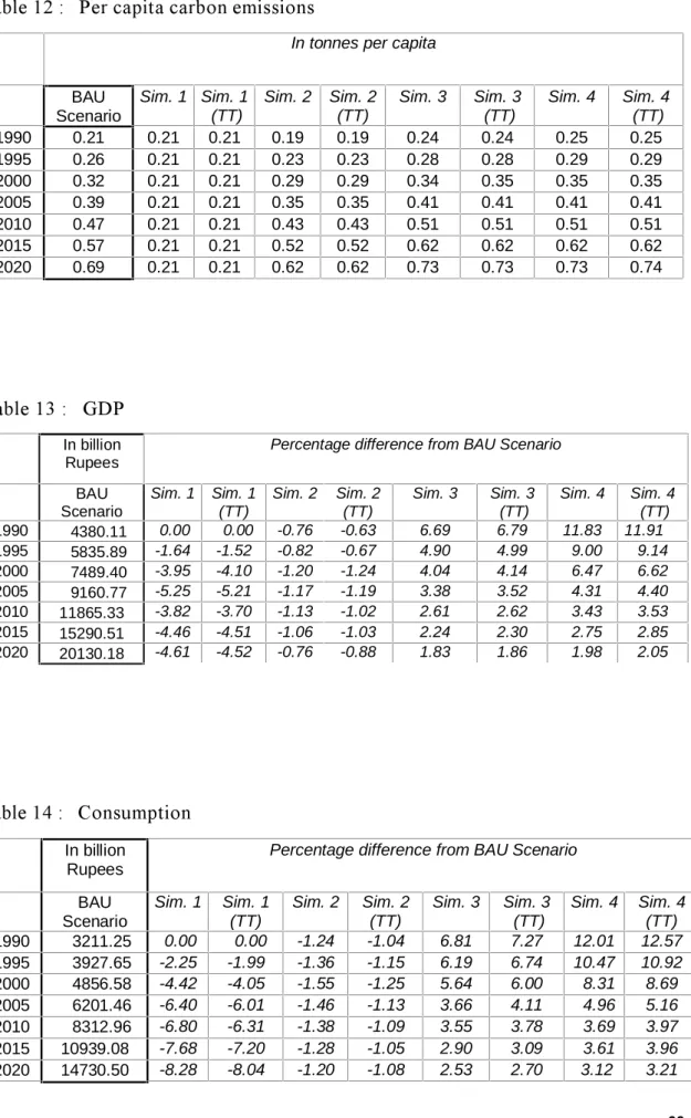
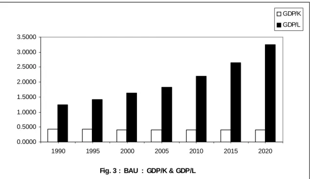
In the BAU scenario, real GDP growth throughout the period 1990-2020 varies in the range 4%-6%. The GDP growth rate, which is 5.7% per year during 1990-95, slows down to less than 5% in the period 1995-2005 (table 6). After that the growth rate picks up again to more than 5% per year till 2020 (figure 2). The driving force of GDP growth in our model comes from growth in the two main exogenous variables - investment and labour supply. In fact, the directional changes and the turning points in the quinquennial GDP growth rates seems to be governed by the exogenously given investment growth rates over the thirty year period. Investment adds to the capital stock, inducing a substitution away from labour into capital. This results in an increase in labour productivity, measured as GDP per unit of labour (figure 3). Growth in labour productivity coupled with the simultaneous growth in labour supply is what provides the main impetus to GDP growth.

3.2 Poverty ratio

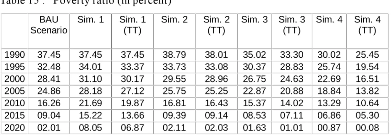
The poverty ratio in the BAU scenario declines from 37.5% in 1990 to 2% in 2020 (table 15). However, the noteworthy fact is that the decline in poverty ratio is very much linked to the growth in GDP. That is to say, with the GDP growing faster after 2005, the decline in poverty also speeds up. In the first 15-year period, 1990-2005, the poverty ratio declines quinquennially by about 4-5 percentage points; in the later 15-year period 2005-2020 it declines quinquennially by about 7-8 percentage points.

13 _{Since Indian database is on an annual basis, we solved the model annually for thirty years. However, the}

results are reported for five-year intervals. This is because, results presented on a year-to-year basis for thirty years, would not be amenable to any meaningful analysis.

(24)

3.3 Energy use

Total energy use increases by about 320% over the 30-year period 1990-2020. However, the annual growth rate of energy use along with the annual growth rate of GDP declines each quinquennium until 2005, with the decline being sharper in case of the former after 2005 (table 7). Increased employment of capital in the production process as well as modest autonomous energy efficiency improvement results in an economy of the energy inputs in the production process as reflected in the declining energy use per unit of GDP.

3.4 Carbon emissions

Total carbon emissions in the period 1990-2020 rise from 168 million tonnes to 559 million tonnes at an average rate of 4.1% per year (table 6). However, the growth rate is not uniform. It drops from more than 4% in the pre-2005 period to less than 4% in the post 2005 period. This is largely explained by the decline in the energy-GDP ratio after 2005 (table 7). In the Indian economy carbon is emitted predominantly - as much as 72% of the total emissions - from the combustion of coal. The share of coal in the total emissions remains unchanged throughout the period (table 10).

In assessing Indias contribution to global carbon emissions, it is important to look at the per capita carbon emissions14_{. Indias per capita emissions in 1990 turn out to be}

0.21 tonnes. It increases quite rapidly over the 30-year period and goes up to 0.69 tonnes by the year 2020 (table 12). Even this level of per capita emissions is considerably less than the global per capita emissions which are approximately 1 tonne per year. 4. Policy Simulations

We develop eight alternative policy scenarios for two basic policy instruments for carbon emission reduction - domestic carbon tax and internationally tradable permits based on equal per capita emissions allocation.

For the carbon tax policy we have four policy scenarios - simulations 1, 1(TT), 2 and 2(TT). Policy simulations 1 and 2 deal respectively with the two cases of fixing the carbon emission at the 1990 level all through the 30-year period, and of 10% annual reduction in emissions, with 2 variants in each - one in which the carbon tax revenues are recycled to the households like additional government transfers, i.e., the across-the-board transfers case, and the other in which the tax revenues are exclusively transferred to a target group comprising of the four lowest income deciles - i.e., the targeted transfers case. For internationally tradable permits, we have again four policy scenarios - simulations 3, 3(TT), 4 and 4(TT) - representing the same 2 variants, with the difference that instead of carbon tax revenues, we have, in this case, revenues earned from the sale of permits. For the policy scenarios 3 and 3(TT), the emissions quota is fixed at 1 tonne per capita14_{based on 1990 population as suggested}

by Parikh and Parikh (1998), who have argued that this would ensure equity between developed and developing countries and simultaneously discourage the latter from increasing their population.

14_{Note that the per capita emissions have been calculated on the basis of the 1990 population for all the}

years, so that a higher population in the years subsequent to 1990 is not allowed to undermine the total emissions in the economy.

(25)

The permit price for the simulations 3 and 3 (TT) is exogenously given to be US$ 6 per tonne of carbon emission, which is Rs 100 per tonne at the 1989-90 exchange rate of Rs 16.60 per dollar. In reality, the permit price will emerge from a global trading system of permits, which, for example, has been modeled by Edmonds et al (1993) in the SGM. However, ours is a country-specific exercise focusing on how it stands to gain or lose from an internationally tradable regime of permits. We, therefore, take the world market price of permits as given, but do consider alternative permit prices in different policy simulations. Hence, the policy simulations 4 and 4(TT) are simply repeat exercises of simulations 3 and 3(TT) respectively, with the permit price exogenously fixed at Rs 200 per tonne.

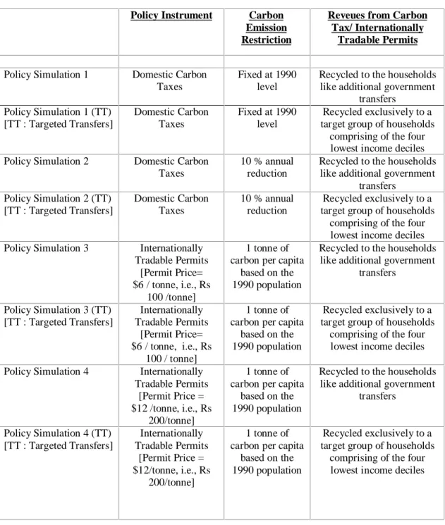
The eight policy simulations are summarized in table 3 given below. Table 3 : The policy simulations

Policy Instrument Carbon Emission Restriction

Reveues from Carbon Tax/ Internationally

Tradable Permits

Policy Simulation 1 Domestic Carbon Taxes

Fixed at 1990 level

Recycled to the households like additional government

transfers Policy Simulation 1 (TT) [TT : Targeted Transfers] Domestic Carbon Taxes Fixed at 1990 level Recycled exclusively to a target group of households

comprising of the four lowest income deciles Policy Simulation 2 Domestic Carbon

Taxes

10 % annual reduction

transfers Policy Simulation 2 (TT) [TT : Targeted Transfers] Domestic Carbon Taxes 10 % annual reduction Recycled exclusively to a target group of households

comprising of the four lowest income deciles Policy Simulation 3 Internationally

Tradable Permits [Permit Price= $6 / tonne, i.e., Rs

100 /tonne]

1 tonne of carbon per capita

based on the 1990 population

transfers Policy Simulation 3 (TT) [TT : Targeted Transfers] Internationally Tradable Permits [Permit Price= $6 / tonne, i.e., Rs 100 / tonne] 1 tonne of carbon per capita

Recycled exclusively to a target group of households

comprising of the four lowest income deciles Policy Simulation 4 Internationally

Tradable Permits [Permit Price = $12 /tonne, i.e., Rs

200/tonne]

1 tonne of carbon per capita

transfers Policy Simulation 4 (TT) [TT : Targeted Transfers] Internationally Tradable Permits [Permit Price = $12/tonne, i.e., Rs 200/tonne] 1 tonne of carbon per capita

Recycled exclusively to a target group of households

comprising of the four lowest income deciles

(26)

It would be useful to bear in mind how the economy would adjust to the introduction of domestic carbon taxes (policy simulations 1, 1(TT), 2 and 2(TT)) and internationally tradable permits (policy simulations 3, 3(TT), 4 and 4(TT)) before going into a detailed discussion of the eight policy scenarios.

A carbon tax results in price increases for each of the fossil fuels coal, refined oil and natural gas. The extent of price increase in case of each of these fuels is determined by the carbon content of the respective fuels. The price increase is largest for coal because coal has the highest carbon content, and smallest for natural gas which has the lowest carbon content. Producers respond by switching from coal towards refined oil and natural gas as a source of energy. At the same time, higher energy prices force a reduction in overall energy use. Carbon emissions are reduced on account of both fuel switching and overall reduction in fuel use. Usually (inter-fossil-fuel substitutions elasticities being low), the fuel reducing effect dominates over the fuel switching effect, resulting in a retardation of GDP growth. Typically, the adverse effect of reduced energy use on GDP growth diminishes over time as energy efficiency improvement coupled with a higher capital intensity in the production process results in a declining energy use per unit of GDP. Typically also, the slowdown in consumption growth is more severe than that in case of GDP growth. When production activity goes down, labour demand and wages decline leading to a fall in personal incomes (unless the addition to personal income from the recycled carbon tax revenue is large enough to offset this fall). Moreover, higher energy prices end up as higher prices for consumer goods, thus lowering real consumption.

With the introduction of internationally tradable permits with equal per capita emissions, India will most likely turn out to be a net seller of permits. A carbon emission quota of 1 tonne per capita based on the 1990 population of 810 million effectively means an upper limit of 810 million tonnes of total carbon emissions for the Indian economy. Looking at the carbon emissions in the BAU scenario (table 9), it is easy to see that India will be a net seller of tradable permits for the next two or three decades. That is, countries with high per capita emissions would purchase permits from countries with low per capita emissions, such as India. That would in effect imply a transfer of wealth into India.16_{The total revenue from the sale of permits in the international market for}

permits is recycled to the households as transfer payments from rest of the world. These transfer payments are akin to an autonomous increase in consumption demand (like an increase in government expenditure), and, therefore, result in a higher demand-driven GDP growth. Higher incomes boost consumption further, so that consumption rises faster than GDP. However, over time as the economy gets close to the upper limit of 810 million tonnes of total carbon emissions, the revenue earned from the sale of permits will shrink, and the GDP gains will become progressively smaller. In fact, in not so distant a future, the economy will turn around from being a net seller of permits to a net buyer of permits.

It may be mentioned that, for our policy scenarios concerned with Indias participation in a regime of internationally tradable permits with equal per capita emissions, we are

16_{A net buyer of permits would amount to a transfer of wealth out of India, but that eventuality does not}

(27)

assuming that the emission permit payments take place through the government, and the latter decides to recycle these to the consumers, rather than producers. Till India is a low per capita emissions country (i.e., till its per capita emissions remain below 1 tonne, the world average) it need not give priority to curbing emissions, but to income distribution and poverty etc. Subsequently, it can switch priorities. That is our view, and our policy scenarios 3, 3(TT), 4, 4(TT) emanate from this view.17

We now turn to an appraisal the policy scenarios. A summary of the key results of the policy simulations are presented in the tables 4 and 5 (Appendix 1). In these tables, selected variables GDP, consumption, aggregate carbon emissions, per capita carbon emissions, poverty ratio and the absolute number of poor of the various policy scenarios are compared with those of the BAU scenario. Needless to say, henceforth, all comparisons for all the policy simulations have been made with respect to the BAU scenario.

4.1 Policy simulations 1 and 1(TT)

In this simulation the procedure followed is to fix the carbon emission level at the 1990 level and to endogenize the carbon tax rate (which was fixed at zero in the BAU scenario). The sequential equilibrium solution of the model then generates, among other values, the appropriate carbon tax rates for each of the years subsequent to 1990. The tax rates rise from Rs 417 per tonne in 1995 to Rs 2765 per tonne in 2020. The growth rate of the carbon tax rate is lower 2005 onwards, because of the lower energy consumption growth rates in this period (table 8). Carbon taxes raise the price of the fossil fuels differentially the increase in price is maximum for coal which has the highest carbon content, followed by that of refined oil and natural gas (table 9) and thus induce fuel switching. The share of coal in total emissions, which was almost 73% throughout the period in the BAU scenario, declines considerably, particularly after 2005. There are corresponding increases in the share of refined oil. The share of natural gas increases only marginally (table 10). The aggregate emission levels fall relative to the BAU scenario by 19% in 1995 and by 70% in 2020. Cumulative emissions in the 30-year period fall by 50% (table 11). Per capita carbon emissions, based on the 1990 population, also fall drastically. In 2020, it is down to 0.21 tonne per capita while it was 0.69 tonnes per capita in the BAU scenario (table 12).

The energy use and GDP trends of simulation 1 suggest that upto 2000, the fuel-reducing effect dominates, and subsequently fuel-saving becomes more important in determining the impact on GDP18_{. Upto 2000, the decline in GDP is more than that in the use of energy inputs. However,}

from 2005 to 2020, energy use declines much faster than GDP. After 2005, the energy-GDP ratio in simulation 1 is significantly lower than that in the BAU scenario (table 7).

17_{Some analysts would want the emission permit revenues to be recycled to producers, who would then}

invest them in new technology with lower carbon emissions. That would be another policy scenario which we have not done in this study. However, it can be done in this model with some changes.

18_{When carbon taxes are imposed , fuel inputs become costly. So, the immediate impact is a reduction in the}

use of fuels leading to a large decline in output. As a consequence, energy-output ratio goes up. This is known as fuel-reducing effect. However, over time the economy adjusts by indulging in more efficient use of fuels. This results in a decline in the energy-output ratio. This is known as the fuel-saving effect.

(28)

Losses in consumption are higher than losses in GDP even though the carbon tax revenues are recycled to the consumers (table 14). This is because the reduced economic activity (reflected in a lower GDP) results in a decrease in the demand for labour and wages causing disposable personal incomes to fall. Moreover, higher energy prices are passed on to consumers through higher consumer goods prices which in turn lower real consumption. The addition to household incomes from the recycled carbon tax revenues are not sufficient to compensate for the fall in their incomes.

The poverty ratio, i.e., the percentage of poor below the poverty line, in simulation 1 increases drastically and progressively from 1995 to 2020. In the BAU scenario, the poverty ratio is 32% in 1995, but declines to 2% in 2020. In simulation 1, the poverty ratio is 34% in 1995 and declines to only 8% in 2020 (table 15). In other words, the number of poor in 2020 in scenario 1 is 4 times the number of poor found in the BAU scenario during the same year (table 16).

In the targeted transfers case of scenario 1 (TT)19_{, the poverty ratio improves a little}

vis-à-vis the across-the-board transfers case of scenario 1. However, in relation to the BAU scenario, it is progressively higher from 1995 to 2020 (table 15). Moreover, the number of poor in the year 2020 under scenario 1(TT) is almost 3.4 times that in the BAU scenario in the same year (table 16).

Policy simulation 2, on the whole, is a milder version of policy simulation 1. In simulation 1, the average annual reduction in carbon emission works out to be 50%, while, in simulation 2, the annual reduction in carbon emissions is fixed to be only 10% (table 11). Per capita emissions, fall progressively from 1990 to 2020. As compared to the BAU scenario, they are 0.02 tonnes less in 1990 and 0.07 tonnes less in 2020 (table 12).

Expectedly, the carbon tax rates in simulation 2 are of much lower orders of magnitude. The carbon tax rate is Rs.218 per tonne in 1990, rises a little in 1995, and, thereafter, declines gradually to Rs.174 per tonne, because of lower energy consumption growth rates in the latter period (table 8). Energy prices also increase moderately (table 9). GDP and consumption losses in scenario 2, as compared to the BAU scenario, are of much lower orders of magnitude than those in scenario 1 (tables 13 and 14). However, consumption losses are more than GDP losses as in scenario 1. In scenario 2, GDP losses vary from 0.75% to 1.20%, while consumption losses vary from 1.20% to 1.55%.

19_{Note that for simulation 1(TT), and likewise for all other TT versions of the remaining 3 simulations, the}

results are discussed for poverty ratio and the number of poor only. This is because the figures for the macro variables in case of the targeted transfers versions of the simulations do not differ much from those in their respective across-the-board transfers versions.

(29)

The poverty ratio in scenario 2 increases only marginally with respect to the BAU scenario. It increases by 1.34 percentage points in 1990, and by only 0.1 percentage point in 2020 (tables 4 and 5). However, the real adverse impact of simulation 2 on poverty comes out in terms of the number of poor. The number of poor in simulation 2, relative to the BAU scenario, increases by 3.58% in 1990 and 4.89% in 2020 (tables 4 and 5).

Under targeted transfers of simulation 2(TT), the poverty scenario is much less adverse than under simulation 2. Poverty ratio, as compared to that of the BAU scenario, increases by 0.56 percentage point in 1990, and by only 0.02 percentage point in year 2020 (tables 4 an 5). The number of poor in simulation 2(TT), compared to that in the BAU scenario, increases by 1.49% in 1990, and by only 0.92% in 2020 (tables 4 and 5). The results of this simulation clearly show that the costs to GDP and poverty reduction imposed by a carbon tax can be reduced to a great extent by moderating the carbon emission reduction target and at the same time recycling the carbon tax revenues to those living below the poverty line.

In policy simulation 3, the carbon emission quota is fixed at 1 tonne per capita based on the 1990 population of 810 million. In other words, the maximum permitted total emission of carbon is fixed at 810 milllion tonnes annually for the Indian economy. For every tonne of carbon emitted less than the permitted 810 million tonnes, the Indian economy earns $6, which is Rs100 at the base-year exchange rate, through the sale of a permit in a global market of permits, and the total revenue form the sale of permits is recycled to the households as transfers from the rest of the world.

The exact procedure followed in this simulation is to fix an upper bound for total emissions - i.e., 810 million tonnes for each year. The actual total emission of carbon turns out to be much less than the upper bound for each period (The upper bound is not binding in any of the years). The difference between the permitted emissions and the actual emissions is then multiplied by the permit price to arrive at the total revenue from the sale of permits, which is then recycled to the households like additional transfer payments from the rest of the world. In the process, the model generates a set of equilibrium values for GDP, consumption, poverty ratio etc.

In simulation 3 the carbon emissions increase relative to the BAU scenario. The increase in emissions is almost 14% in the year 1990, but, in the later years, declines to be in the range of 5.50-9.00% (table 11). Per capita emissions also increase throughout the period, with the increases being in the range of 0.02-0.04 tonnes (table 12). However, what needs to be noted is that, even in the last year, 2020, per capita emissions are only 0.73 tonnes, which is less than the world average of 1 tonne per capita.

The infusion of additional transfer payments from the rest of the world, in the form of permit revenue, leads to substantial increases in GDP and consumption in this simulation. GDP increases by 6.7% in the year 1990. However, in the later years, GDP increases are progressively smaller. In the final year, 2020, GDP increases by only 1.8%. The

(30)

consumption gains are higher than the GDP gains in each of the periods (tables 13 and 14). Apart from the increases in consumption resulting from the increased transfers to households, there are second-round increases in consumption when there is additional income generated from the demand-induced increase in production activities.

The poverty ratio declines significantly in scenario 3. It declines by 2.43 percentage points in the year 1990, and by 0.38 percentage points in the year 2020 (tables 4 an 5). The number of poor, relative to the BAU scenario, decreases by 6.5% in 1990, and by 18.8% in the year 2020. That is, in the final year, 2020, the number of poor is only 21.24 million in this simulation, as compared to 26.15 million in the BAU scenario (table 5).

Poverty declines even faster under the targeted transfers version of simulation 3. The number of poor in this scenario, compared to the BAU scenario, declines by 11% in 1990 and by 50% in 2020. By the year 2020, the number of poor in this simulation is only 13.18 million, i.e., half of