Dynamic Integrated Scheduling of Hard Real-Time,
Soft Real-Time and Non-Real-Time Processes
†
Scott A. Brandt
Scott Banachowski
Caixue Lin
Timothy Bisson
Computer Science Department
University of California, Santa Cruz
sbrandt,sbanacho,lcx,tbisson
@cs.ucsc.edu
Abstract
Real-time systems are growing in complexity and real-time and soft real-real-time applications are becoming common in general-purpose computing environments. Thus, there is a growing need for scheduling solutions that simultaneously support processes with a variety of different timeliness con-straints. Toward this goal we have developed the Resource
Allocation/Dispatching (RAD) integrated scheduling model
and the Rate-Based Earliest Deadline (RBED) integrated multi-class real-time scheduler based on this model. We present RAD and the RBED scheduler and formally prove the correctness of the operations that RBED employs. We then describe our implementation of RBED and present re-sults demonstrating how RBED simultaneously and seam-lessly supports hard real-time, soft real-time, and best-effort processes.
1. Introduction
Modern embedded, special-purpose and general-purpose computing systems are becoming increasingly complex. At the same time, the traditional notions of best-effort and real-time processing have fractured into a spectrum of pro-cessing classes with different timeliness requirements in-cluding best-effort, desktop multimedia, soft real-time, firm real-time, adaptive soft real-time, rate-based, and traditional hard real-time. Many different schedulers support the im-portant characteristics of each of these classes. However, none of them fully integrates the processing of these het-erogeneous classes into a single scheduler.
Hierarchical systems can support multiple classes of pro-cesses, but do so through potentially complex hierarchies of schedulers. Because hierarchies partition the system among
† This research was supported by Intel Corporation, a Department of Energy High Performance Computer Science Fellowship, and the USENIX Association
different schedulers, this strategy of integrating multiple schedulers may limit the ability to trade off merits of in-dividual processes of different classes, and may compli-cate slack management. In contrast, a unified, integrated scheduling approach may make decisions while fully aware of the state of all processes.
To address this issue, we present a general model of real-time scheduling called Resource Allocation/Dispatching
(RAD). RAD explicitly separates the management of the
amount of resources allocated to each process from the tim-ing of the delivery of those resources. This separation al-lows the resource management to be precisely tailored to the needs of the individual processes. By allowing these two aspects of scheduling to be varied dynamically and inde-pendently, the RAD model fully captures the very different needs of the different real-time and non-real-time schedul-ing classes.
As a proof-of-concept, we have developed the
Rate-Based Earliest Deadline (RBED) scheduler. RBED is a
RAD scheduler that provides fully integrated scheduling of hard real-time, soft real-time, and best-effort processes. It uses dynamic rate-based resource allocation and dynamic period adjustments for fine-grained control of both resource amounts and timing.
2. The RAD CPU Scheduling Model
Traditional non-real-time CPU schedulers serve two roles in CPU resource management: resource
alloca-tion and dispatching. Resource allocaalloca-tion determines how
much of the resource to give each process, while dispatch-ing determines when to give the allocated resources to each process. Historically, the extreme efficiency require-ments imposed on schedulers demanded unified approaches that merge these two important aspects of schedul-ing into a sschedul-ingle mechanism. However, the recent rapid increase in CPU speeds enables the use of slightly more so-phisticated scheduling mechanisms without significantly impacting overall system performance.
Although all schedulers implicitly address both resource allocation and dispatching to some degree, most do not explicitly separate their management and allow them to be independently adjusted at run-time. However, differ-ent classes of applications exhibit very differdiffer-ent character-istics with respect to both resource allocation and deliv-ery requirements. Dynamically and independently manag-ing these two quantities thus enables the integrated schedul-ing of these different classes of processes.
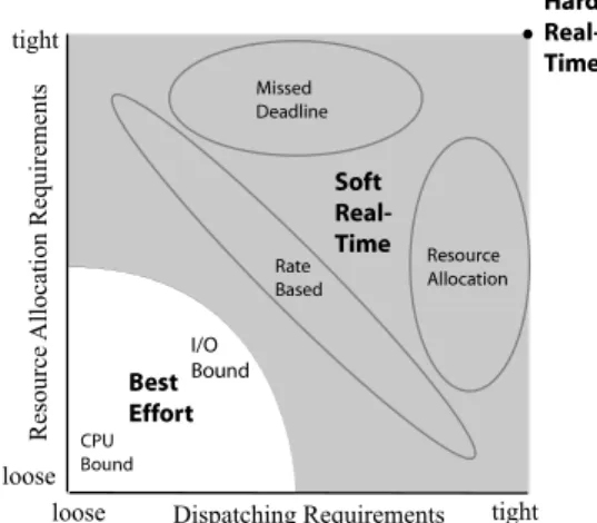
Figure 1 presents a conceptual diagram of the resource allocation and dispatching requirements of each class of processes. Each axis represents the relative tightness of the requirements of the classes of processes, ranging from very loose to very tight. Hard real-time processes have extremely tight resource allocation and dispatching requirements. By contrast, best-effort processes have very loose resource al-location and dispatching requirements, generally being able to run as slow and sporadically as necessary without be-ing thought of as havbe-ing failed. However, even within best-effort scheduling there is variation in terms of these require-ments. Non-interactive CPU-bound processes need greater amounts of CPU, but within very broad parameters they can use it in any size increments and at any time. I/O-bound pro-cesses, especially interactive ones, use relatively little CPU but need to receive it quickly once they have unblocked in order to provide good interactive responsiveness.
loose tight loose tight Dispatching Requirements Resource Allocation Requirements t d e t e I/O nd CPU ! " nd #!$&% !"'( e )** !(+, ion -/.% sed 0$1+ dline #!+, e +&% ed
Figure 1: Resource allocation and dispatching re-quirements for different types of processes
Between hard real-time and best-effort lies a broad class of applications and systems referred to as soft real-time (SRT). This includes a variety of different systems with varying properties, all of which share the common prop-erty that resource allocation and/or dispatching require-ments are looser relative to hard real-time. Figure 1 divides these into three broad sub-categories—Missed Deadline Soft Time (MDSRT), Resource Adaptive Soft
Real-Time (RASRT), and Rate-Based (RB)—depending upon which constraints are relaxed. MDSRT is real-time process-ing in which the time constraint is softened such that real-time processes may miss their deadlines in varying percent-ages or by varying degrees when all deadlines cannot be met [12, 17, 18]. By contrast, RASRT is real-time process-ing in which the resource allocation constraint is softened while attempting to minimize the number and amount by which deadlines are missed [4, 5, 12, 25]. In Rate-Based processing both resource allocation and dispatching can vary, but not completely independently; if more resources are provided a longer time may elapse before resources are again allocated and if less resources are allocated a shorter time may elapse before resources are again allocated [8, 11]. As this discussion demonstrates, the RAD model cap-tures the important differences between these different classes of processes. The key to developing a fully inte-grated multi-class real-time RAD scheduler thus depends upon the development of mechanisms that will support dif-ferent and varying degrees of requirements on both the resource allocation and dispatching. The Rate-Based Ear-liest Deadline (RBED) scheduler was developed to do exactly this.
3. The Rate-Based Earliest Deadline (RBED)
Scheduler
RBED is a RAD scheduler for hard time, soft real-time, and best-effort processes. RBED resource allocation is accomplished via dynamic process rate adjustment. RBED dispatching is accomplished via dynamic application period adjustment. Based on the specific processing requirements of each process and the current system state, RBED assigns a target rate of progress and period to each process in the system. Both are enforced at runtime by a modified EDF scheduler that dispatches processes in EDF order but inter-rupts them via a programmable timer when they have ex-hausted their alloted CPU for the current period.
RBED allocates resources to processes as a percentage of the CPU such that the total allocated to all processes is less than or equal to 100%. Hard real-time processes have a period p and worst-case execution time e and are either granted their desired rate e2 p or are rejected if insufficient
resources are available. Soft real-time processes are given their desired rate e2 p if possible, or are given less,
possi-bly based upon a QoS specification if one is available. Like hard real-time processes, rate-based processes are given the rate that they request if possible, or are rejected. The rate of each best-effort process is a calculated share of the rate that remains after the rates of the other processes in the sys-tem have been determined. A reservation mechanism can guarantee that a minimum or maximum allocation is avail-able to a particular class of processes, ensuring, for
exam-ple, that there are always some resources available to the best-effort processes.
RBED assigns periods in cases where application do not already have them. Hard and soft real-time tasks have pre-specified periods. Periods for rate-based tasks are de-termined based on the processing requirements of the par-ticular task. At deadlines, a process’ desired and actual re-source usage are equal, and so the difference between the desired and actual resource usage at non-deadline times are bounded by the choice of period. Thus the necessary pe-riod for rate-based tasks can be determined directly by the amount they are allowed to stray from their target rate. For example, in an audio player application this is a function of the data sampling rate and the size of the audio device’s memory buffer. For best-effort tasks, a semi-arbitrary pe-riod is assigned to ensure a high degree of responsiveness, when needed.
Thus, by allocating the resources appropriately, choos-ing appropriate deadlines, and uschoos-ing a programmable timer, RBED presents to EDF exactly what it wants and guar-antees that all deadlines are always met, that all rate con-straints are met, and that all processes receive the correct amount of CPU. However, unlike processes in traditional hard real-time systems, the rates of soft real-time and best-effort processes may change as processes enter and leave the system, and the periods of soft real-time processes may change as they adjust to the available resources. The next section provides proofs that we can maintaining the correct-ness of EDF under these conditions.
4. RBED Theoretical Background
Because RBED uses earliest deadline first (EDF) to schedule periodic tasks1, its theory is based on well-known real-time scheduling principles. However, the standard def-inition of EDF and proofs of its correctness and optimal-ity usually assume that the worst-case execution time and the period of a task is fixed during its lifetime, while RBED dynamically adjusts both of these properties. In this section we prove that EDF functions correctly with the dynamically changing rates and periods of RBED.
When either rate or period change (or both), the task un-dergoes a mode change. Previous works describe the con-straints under which either fixed-priority [22, 24] or proportional share [23, 2] scheduling algorithms al-low mode changes. In this section, we determine the impact on schedulability when a task changes mode at ar-bitrary times under EDF, and describe the conditions un-der which EDF still guarantees deadlines after a mode change. Understanding these constraints allows us to
cre-1 The terms “task” and “process” are used interchangeably throughout this paper.
ate flexible schedules for the dynamic workloads presented to the RBED scheduler.
We introduce a slightly different task model than sup-plied in the Liu and Layland proof [15]. In the original proof a task consists of a sequence of periodically released jobs whose deadlines equal their release times plus the task pe-riod. The RBED task model is the same, except that each job in a task may have a different period. We first show that under this model an EDF schedule remains feasible as long as the utilization is constant, and then we relax even this requirement. We use the following notation: a task Ti con-sists of sequential jobs Ji3k, where each job has a release
time ri3k, period pi3k, deadline di3k, and worst-case execution
time ei3k. For any k, utilization
2u
i 4 ei3k
2 pi
3k, ri3k4 di3k5 1,
and di3k 4 ri3k6 pi3k. The total utilization of the system is
U 4 ∑i
7 Tui, where T is the set of all tasks. In some cases,
subscripts are dropped if the meaning is obvious.
Theorem 1 The earliest deadline first (EDF) algorithm
will determine a feasible schedule if U 8 1.
Our modified task model does not invalidate this theory; for reference a similar proof using the new task model is provided in Appendix A. The benefit of the new model is that it supports arbitrary period changes at job deadlines. The restriction that period changes occur only at deadline boundaries is relaxed below.
When a job completes and a new job is released with a different period, it is equivalent to the task leaving at the same instance that a new task of the same utilization en-ters the system. In this sense, it is safe to consider the uti-lization of a departing task as part of the unallocated CPU (19 U ) when its last deadline is reached.
Corollary 1.1 Given a feasible EDF schedule, at any time
a task with utilization8;:19 U< may enter the system and
the schedule remains feasible.
The proof is implicit in the proof for Theorem 1, because it holds for tasks of arbitrary starting times.
4.1. Increasing Utilization or Period
Theorem 2 Given a feasible EDF schedule, at any time a
task Timay increase its utilization by an amount up to 19 U
without causing any task to miss deadlines in the resulting EDF schedule.
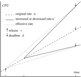
Figure 2 shows the effect of increasing the utilization of an already released job. At time t, the instantaneous uti-lization of the task increases from u to u=, but over the
life of the job, the job effectively consumes a utilization
ue f f ective 4 :>:t9 r<@? ui 6 :d9 t<@? u=< 2 :d9 r<.
2 Utilization is synonymous with rate. We are using the term utilization and the symbol u in the proofs instead of rate and r, because the sym-bol traditionally refers to release time.
time release deadline effective rate CPU d
increased or decreased rate
r t (time of mode change)
u
original rate
u’
d r
Figure 2: Increasing or decreasing the rate of an already released job
The proof uses Corollary 1.1; the schedule resulting from increasing the utilization of a task is equivalent to a sched-ule in which another task having the same deadlines en-ters the system. Assume that at time t task Ti, which al-ready released a job at time ri, wishes to increase its utiliza-tion to u=
i4 ui6 ∆, where∆
8 19 U . To meet its deadline
with the new utilization, it requires e=
i4 ue f f ective :di9 ri< 4 ui:t9 ri< 6 :ui 6 ∆
<A:di9 t< CPU in the interval :ri
BdiC. At
this time, introduce task T=
i with period p=
i4 di
9 t and
uti-lization∆. By Corollary 1.1, the schedule remains feasible. During the interval:t
BdiC, the CPU assigned to both Tiand
T=
i is used for Ti, and over the interval :ri
BdiC the total CPU
allocated to Ti equals ui:di9 ri< 6 ∆ :di9 t< 4 e = i. For sub-sequent periods, the tasks Ti and T=
i may be merged into a single task of utilization ui6 ∆.
Theorem 3 Given a feasible EDF schedule, at any time a
task Timay increase its period without causing any task to
miss deadlines in the resulting EDF schedule.
The task model described in Theorem 1 allows subse-quent jobs to have different periods. We now consider in-creasing the period of an already released job Ji3k,
effec-tively extending its current deadline from di3kto d
=
i3k
. If, in the unchanged schedule, Ji3kis followed by a job released at
di3kwith period pi3kD 14 d
=
i3k
9 di
3k, the schedule is feasible.
In this schedule, the total CPU consumed by both jobs over the interval :ri
3kBd
=
i3k
C is the same as if the original period
of Ji3kwas the new period. Instead of releasing the jobs
se-quentially, we wish to simply extend the current job’s dead-line, and ensure that changing it on-the-fly does not cause another task to miss a deadline due to changes in dispatch order.
A simple “interval swapping” argument shows that EDF does not miss any deadlines in the new resulting schedule:
all jobs with deadlines before di3kwill execute in the same
intervals before and after the period change. Any jobs with deadlines at or after di3k, but before d
=
i3k
, will be dispatched in earlier intervals under the new schedule, so are not at risk of missing deadlines. And because EDF is work conserv-ing, any jobs with deadlines after di3k that receive CPU in
the interval:t
Bd
=
i3k
C under the previous schedule receive the
same amount of CPU in this interval of the new schedule.
4.2. Decreasing Utilization or Period
As long as the requested utilization does not exceed the CPU bandwidth, increasing the utilization or period of an already released job is unconstrained. This is not the case when decreasing utilization or period. For example, in an EDF schedule it is possible for a task to meet its deadline without any laxity. Clearly, this task cannot meet an earlier deadline, as it just barely makes its existing deadline. This section describes the conditions that allow decreasing the utilization or period of an already-released job. These con-ditions depend only on the state of the task, so that it may change mode without needing to determine the state of any other tasks.
The lag of a job is the difference between its ideal and actual service time. The ideal service time is the amount of CPU the job receives assuming ideal (fluid) scheduling, and equals u:t9 r<. At t, if the job actually consumes x CPU
since time r, lag:t
Bx
<
4 u
:t9 r<E9 x. A negative lag means
a task is proceeding ahead of its ideal service time. The lag concept is often used when characterizing algorithms that approximate fair sharing—because proportional share algo-rithms bound lag, it is useful for proving mode change con-straints.
If a task meets its deadline, then at its deadline it has zero lag (lag:r
6 pBe < 4 e 2 p ::r 6 p <F9 r<G9 e 4 0).
Depend-ing on the schedule, there may be several times durDepend-ing a job’s lifetime that lag is zero. If the task leaves the system when its lag is zero, the utilization may be immediately re-claimed for use by any task.
Lemma 1 Given a feasible EDF schedule, if a task with
zero lag leaves, its utilization may be used by a new task, and the resulting EDF schedule remains feasible.
At a task’s deadline, this is already known to be true. Here we sketch the proof when a task is not at its dead-line. If job Ji3nhas zero lag at time t, its current service time
is xi3n4 ui
:t9 di
3n5 1
<. At this time the current job leaves
(and hence has no deadline to miss) and the task releases a new job of period pi3nD 1. At the deadline of a later job Ji3m,
the total service time requested by the task is (withφiequal to the time of the first release):
uiHdiI1J φiK!L uiHdiI2J diI1KLNMOMOM L uiHtJ diInP 1K
L uiHdiInQ 1J tKLNMOMOM L uiHdiImJ diImP 1KSR uiHdiImJ φiK
The remainder of the proof follows that of Theorem 1 supplied in Appendix A. The total service demand of the
task remains the same as in Equation (A.1), so a missed deadline requires U T 1, a contradiction.
A task may reduce its utilization at any time, without affecting the feasibility of the existing task set, because the overall service time is reduced. However, because the scheduler assumes that jobs will complete their periods, it is not apparent that the utilization freed by this task is avail-able to other tasks until its existing period completes. How-ever, if the utilization of a task is decreased within a con-straint, we see that EDF can guarantee the freed utilization immediately to other tasks.
Theorem 4 Given a feasible EDF schedule, if at time t
task Ti decreases its utilization to u=
i 4 ui
9 ∆ such that
∆8 xi2 :t9 ri<, the freed utilization∆is available to other
tasks and the schedule remains feasible.
Figure 2 shows the effect of decreasing the utilization of an already released job. At time t, the instantaneous uti-lization of the task decreases from u to u=, but over the
life of the job, the job effectively consumes a utilization
ue f f ective 4
::t9 r<@? ui
6
:d9 t<@? u=U< 2 :d9 r<.
The schedule described in Theorem 4 is equivalent to the following hypothetical EDF schedule, which is feasible: At time ri, imagine that instead of Ti releasing a job with ui, two tasks release jobs: Ta’s job has deadline diand utiliza-tion uaand Tb’s job has deadline t and utilization ub, where
ua6 ub4 ui. At time t Tbmay leave the system and ubis
available for use by other tasks. The service time received by Tbat t is ub:t9 ri<.
In the actual schedule, at time t we wish to make∆of task T=
is utilization available to another task. This is equiv-alent to letting a portion of the task leave the system, as though it met a hypothetical deadline. The service time of
Tiat t must exceed the service time of the hypothetical task leaving the system, i.e. xi V ub
:t9 ri<. Letting ub
4 ∆, if
∆8 xi
2
:t9 ri<, the resulting schedule is feasible if another
task uses∆at t.
Theorem 5 Given a feasible EDF schedule, if a currently
released job Ji3nhas negative lag at time t (the task is
over-allocated), it may shorten its current deadline to at most xi2 ui, and the resulting EDF schedule remains feasible.
Lowering the period is possible if the task is currently over-allocated. According to Lemma 1, if the lag equals zero, then it is safe to change the deadline. Note that if the task is over-allocated, it will reach zero lag by idling for9 lag:t
Bxi
< 2 uiunits of time. Thus, the deadline of a job
may be reduced to any value of d=
isuch that its current ser-vice time does not exceed its utilization, i.e. xi2 d=
i 8 ui, so
d=
i V xi
2 ui.
When the deadline is decreased to d=
i, tasks with dead-lines before d=
i are unaffected. If in the original schedule no CPU is allocated to Ji3nbetween t and d
=
i, then the new
schedule is feasible, because it is exactly the same schedule produced if a period change occurs at d=
i, when it is permis-sible by Lemma 1. Thus, tasks at risk of missing deadlines are those with deadlines after d=
ibut before di, as they would preempt Tiin the original schedule. Note that if any of these jobs were released before ri3n, then Ji3nwould not have
re-ceived CPU before them, and so it would not have nega-tive lag; therefore any jobs at risk were released in the inter-val :ri
3n
BdiC. The proof proceeds as follows: if any of these
“at risk” tasks miss a deadline after d=
i, the utilization ex-ceeds 1, which is a contradiction. The details are provided in Appendix B.
In some cases it may be feasible to lower the deadline of a task even if it has positive lag. However this is not al-ways so, for example when the task has no laxity. To deter-mine if a task with positive lag may safely reduce its period requires knowledge of the state of other tasks in the system, because it must be determined if tasks with pending dead-lines have enough slack to potentially change dispatch or-der; it is therefore simpler to use the loose constraints of Theorem 5.
4.3. Superposition of Mode Changes
The above section examines the effect of a single mode change of either utilization or period, while the other pa-rameter is held constant. It is possible for a task to instan-taneously change both the utilization and period, and the bounds are determined by a piecewise combination of the above rules. When determining the bounds of feasibility, it is useful to apply the change to the less constrained param-eter first.
Increasing Utilization and Period Increasing either period
or utilization is unbounded by the task state, so it is always feasible to do both operations as long as U 8 1.
Decreasing Utilization, Increasing Period Increasing the
period is unbounded, but the amount that utilization may de-crease is a function of service time (Theorem 4). Changing the period has no effect on service time, so the bound that utilization may be lowered depends only on the received service time, and remains the same.
Increasing Utilization, Decreasing Period The amount that
a period may be lowered depends on the new effective uti-lization of the utiuti-lization change. Figure 2 shows that af-ter the job increases its utilization, although the task be-gins processing at its new utilization, for the currently re-leased job the effective utilization is an intermediate value between the old and new period. The effective period of the job is ue f f ective4 u
:t9 r<
6 u
=!:d9 t< 2 :d9 r<, and the bound
on lowering the period of this job is x2 ue f f ective.
Decreasing Utilization and Period If a task is
af-ter lowering utilization it is possible that under the new ue f f ective the lag is no longer positive, and the pe-riod may now be lowered to x2 ue f f ective.
Thus by following the constraints imposed by the above theorems, it is possible to vary the rate and period of pro-cesses as required by RBED while still maintaining the cor-rectness of EDF. This enables the implementation of the RBED scheduler, as discussed in the following section.
5. RBED Implementation
After simulating all of the RBED operations, we im-plemented a proof-of-concept version of RBED in Linux 2.4.20 on an Intel Pentium 4 platform. RBED supports all of the processing classes shown in Figure 1 but due to space limitations this discussion is limited to our support of hard real-time, missed deadline soft real-time, and best-effort processes. The changes to the Linux kernel include less than 550 lines of modified or added code. We added several attributes to the process state structures for RBED book-keeping: process type, period, worst case execution time (WCET), weight, and deadline. We also added two system calls to allow processes to interface with the RBED sched-uler: set rbed scheduler(deadline type, period, WCET) and rbed deadline met(void).
All processes default to the best-effort scheduling class. set rbed schedule() turns a process into a real-time pro-cess. The arguments specify the period, worst-case execu-tion time (WCET), and whether the deadlines are hard or soft. The target resource rate (utarget) of a process is de-fined as WCETperiod. A hard real-time process is guaranteed to receive an actual resource rate (uactual) equal to utarget if enough CPU is available, otherwise the process is not ad-mitted as a real-time process. A soft real-time process re-ceives a uactual equal to its utarget or less, depending on the available resources. Set rbed schedule() returns the amount of utilization available to the process—if a soft real-time task receives less than it requested it may continue, adapt to the available resources, or abort.
Real-time processes call rbed deadline met() when they finish a periodic computation. It returns true or false de-pending upon whether or not the process met its deadline. This allows processes to synchronize their periods using system clocks and to determine if a deadline is missed with-out having to compute the time. If this function is called be-fore a deadline, the process suspends until its next release time. If a soft-real time computation exceeds its WCET, it will call this function after its deadline, in which case it re-turns false, and the application may deal with the missed deadline appropriately.
There are two main components of the RBED scheduler: a resource allocator [14], and an EDF-based dispatcher. The resource allocator sets the periods and WCET of all tasks so
do resource allocation(process p)W
switch(pXtype)W
case Hard real-time:
pXuactual
R p
Xutarget;
break; case Soft real-time:
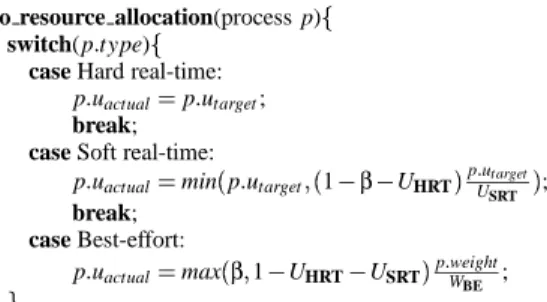
pXuactual R minHp Xutarget Y!H1J βJ UHRTK pZutarget USRT K; break; case Best-effort: pXuactual R maxHβY1J UHRTJ USRTK pZweight WBE ; [\[
Figure 3: Resource allocation pseudo-code. β is the minimum resource rate reserved for best-effort processes.
that the EDF scheduler is never overloaded. The resource al-location component is triggered whenever a process enters or leaves the system or a best-effort process blocks or un-blocks. The algorithm sets uactual for each task according to its requirements. Hard real-time tasks receive their re-quested utilization, soft real-time task receive the leftover CPU, minus the portion of CPU (β) reserved for best-effort processes. Best-effort processes receive utilization in pro-portion to their weights, described in more detail in Sec-tion 5.1. The pseudo-code in Figure 3 describes the alloca-tion policies. In this code, UX4 ∑p
7 Xp
]uactual, where X is
the set of all tasks of type X , and WBE4 ∑p
7 BEp
]weight.
Note that in this calculation we count only runnable best-effort processes – blocked best-best-effort processes have an ef-fective weight of zero.
To ensure a feasible schedule, a process must not overrun its worst-case execution time. RBED uses a one-shot timer to interrupt a task when it consumes its WCET. If a task reaches its WCET, the one-shot timer interrupt handler will preempt the process and advance its absolute deadline to the end of its subsequent period. RBED uses the Advanced Programmable Interrupt Controller, which is capable of bet-ter than microsecond precision with little overhead, for its one-shot timer. This allows the kernel to continue to use the regular programmable interrupt timer for system time ser-vices.
5.1. Scheduling Best-effort Processes
Best-effort schedulers attempt to provide fair allocation of the CPU over the long term. In addition, to improve the responsiveness of I/O-bound applications, they give a short-term “boost” to processes immediately after they block. One goal of the RBED scheduler is to preserve this behavior for best-effort processes.
Unlike real-time processes, best-effort processes lack the time constraints required by deadline-based schedul-ing algorithms. RBED therefore assigns dynamic pseudo-periods to best-effort processes. The period is equal to
rbed schedule()W
1. If RT process enters or leaves and system is overloaded then for all p in RT, do resource allocation(p). 2. Use EDF to dispatch a process.
3. If the selected process p is in BE /*do lazy allocation*/
do resource allocation(p).
4. Clear one-shot timer for the previous process and reset one-shot timer for the selected process. 5. Context switch if needed.
[
Figure 4: Pseudo-code for rbed schedule()
NBE? quantum, where NBEis the number of runnable
best-effort processes and the quantum reflects the scheduling quantum of a time-share system. RBED, like the version of Linux it was implemented in, assigns a default quantum of 60 ms.
Every best-effort process has a weight, which is the rate it consumes CPU relative to other runnable best-effort pro-cesses. Figure 3 shows how RBED maps weight into utiliza-tion. Given uactual, the WCET is NBE? quantum? uactual.
A task’s weight fluctuates depending on its state. When-ever a best-effort process consumes its WCET without blocking, its weight is set to 0. A process that blocks be-fore using its entire WCET retains its weight. When no runnable processes have a nonzero weight, all runnable pro-cess’s weights are set to one, and all blocked processes re-ceive weight 4 weight
2 2
6 6 (which is bounded to a
maxi-mum of 12). The static value 6 provides a boost similar to that of Linux.
In order to avoid frequent resource allocation recompu-tation any time a process enters or leaves the system or a best-effort process blocks or reenters the ready queue, RBED lazily applies the resource allocation algorithm to each best-effort task when it is selected for dispatch. Fig-ure 4 shows the pseudo-code for the scheduler. Parameters of already released jobs are set within the constraints de-fined in Section 4.
When real-time tasks complete the processing for a pe-riod, the next job is not released until the period expires. In our RBED prototype, best-effort tasks are treated dif-ferently: instead of suspending a best-effort job when it consumes its WCET, the next job is immediately released (with the deadline set to the end of its next pseudo-period). This allows best-effort processes to consume all of the dy-namic slack inserted into the schedule by real-time pro-cesses. This approach is similar to the those used in other systems, such as in Portable RK [19], which runs depleted tasks at a low background priority. However RBED does not need to maintain a background scheduling algorithm; the resource allocator only needs to release the task’s next job early, using the later deadline to effect a background priority with no change to the dispatcher or any other tasks’ param-eters. This simple technique distributes the slack among the
best-effort tasks according to their relative weights. How-ever, it does not allow other classes of processes (notably soft real-time) to take advantage of dynamic slack. In the future we plan to examine techniques for making regularly available dynamic slack available to soft real-time processes as well.
6. Performance Measurements
To characterize the performance of RBED, we com-pare it to the Linux scheduler and to a hierarchical EDF/best-effort scheduler we developed called
EDF-Linux. Both Linux and EDF-Linux use the 2.4.20 kernel.
EDF-Linux maintains two ready queues, one for peri-odic real-time tasks, scheduled by EDF, and another for best-effort tasks, scheduled by the default Linux sched-uler whenever the real-time queue is empty. All experi-ments were performed on a standard PC Desktop equipped with a 1 GHz Pentium III processor, 512MB RAM, and a 40GB hard drive. In developing our prototype we have run the system over long periods of time. Our general impres-sion is that the scheduler works well. Best-effort tasks ex-hibit “normal” behavior (with default scheduling quanta of 60 ms, the same as the Linux scheduler) and are never com-pletely starved, real-time tasks meet their deadlines, and soft real-time tasks meet their deadlines or run at lower per-formance levels depending upon the amount of resources available. Below we present a series of snapshots that il-lustrate how RBED performs in practice. For simplicity we have drawn the graphs relative to an origin start-ing at (0,0) even though the snapshots were taken from the middle of longer executions.
Real-time workloads for these tests were generated by a tool we developed to easily generate periodic workloads with different utilization and timing behavior. Given a spec-ification of a desired period and rate (where rate is WCETperiod), the tool generates periodic hard real-time or soft real-time processes with constant or variable (with a normal distri-bution) execution times. We arbitrarily reserve a minimum of 5% of the CPU for best-effort processes, enough to pro-vide a functional interactive system for running command shells during experiments.
Figures 5 shows the performance of the Linux and RBED schedulers when running two best-effort processes, one CPU-bound and one I/O-bound. The CPU-bound pro-cess performs a floating point calculation in a tight loop, while the I/O-bound process repeatedly com-putes for 300 ms then sleeps for 1200 ms. The RBED re-sults are nearly identical to the Linux rere-sults. Figure 6 shows closeup views of the behavior when the I/O-bound process reenters the ready queue after blocking (a con-stant offset was added to the y-axis of the I/O process’s data set to view the two lines in the same axes). Again the
re-sults are nearly identical. When an I/O-bound process blocks, Linux increases its scheduling quantum and pri-ority. When it awakens, the I/O-bound process receives a long quantum of about 110 ms. After this quantum, the I/O-bound and CPU-bound process share the CPU, each us-ing 60 ms quanta. When both quanta expire, they are both replenished to 60 ms. When two processes have equal prior-ity, Linux prefers to avoid a context switch, so the same pro-cess consumes another quantum for a total of 120 ms. The RBED scheduler uses a similar boost formula for sleep-ing best-effort processes, as described in Section 5.1. The I/O-bound process has a weight of 11 when it awakes, and so its WCET is adjusted to :2<A:60<:
11 11D 1
<
4 110 ms.
Af-ter this computation, the weight of the I/O-bound cess is reduced to 1, the same as the CPU-bound pro-cess, and the two processes share the CPU using 60 ms quanta (WCET4 :2<:60< 1 ^ 1D 1_ 4 60). 0 20 40 60 80 100 0 20 40 60 80 100 CPU Time (s) Time (s) I/O process CPU process
(a) Standard Linux scheduler
0 20 40 60 80 100 0 20 40 60 80 100 CPU Time (s) Time (s) I/O process CPU process (b) RBED scheduler
Figure 5: I/O vs. CPU-bound processes on the Linux and RBED schedulers
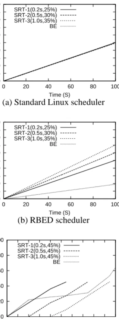
Figure 7 shows multiple soft real-time processes with a single best-effort process. In Figures 7(a) and (b), the three soft real-time processes have (period,rate) equal to (0.2s,25%), (0.5s,30%) and (1.0s,35%). Each of the four processes receive 25% of the CPU under Linux’s scheduling algorithm. In this case, SRT-1 meets its dead-lines, but the other two soft real-time processes miss all of their deadlines. By contrast, RBED ensures that each of the soft real-time processes receives its required
re-0 50 100 150 200 250 300 350 400 450 0 200 400 600 800 1000 CPU Time (ms) Time (ms) I/O process CPU process
(a) Standard Linux scheduler
0 50 100 150 200 250 300 350 400 450 0 200 400 600 800 1000 CPU Time (ms) Time (ms) I/O process CPU process (b) RBED scheduler
Figure 6: Closeup of I/O vs. CPU-bound processes on the Linux and RBED schedulers
sources (25%B30%B30%) and meets all of its deadlines
and the best-effort process receives the remaining re-sources (10%). Figure 7(c) shows how RBED man-ages SRT resources when the system undergoes load changes, due to applications entering and leaving the sys-tem. Initially SRT-1 runs with resource rate of 45% as a best-effort process receives the leftover CPU (55%). Af-ter 40 seconds, SRT-2 enAf-ters and is allocated 45%, while the best-effort rate drops to 10%. At 80 seconds, SRT-3 en-ters and forces the other two soft real-time processes to decrease their resource rates so that the system is not over-loaded. As a result, each soft real-time process receives a resource rate of 31.6%, and the best-effort process re-ceives the best-effort reservationβ. After the 109 seconds the three soft real-time processes begin to leave the sys-tem and the rates of the other processes increase accord-ingly.
Figure 8 shows RBED running two hard real-time processes (20%, 60%), a soft real-time process (pe-riod, rate)=(0.5s,40%), and a best-effort process. The two hard real-time processes receive their required re-sources, unaffected by the presence of the soft real-time or best-effort processes. Because the available resource for the soft real-time process is less than 40%, the sched-uler dynamically extends its period, thus reducing its
0 5 10 15 20 25 30 35 40 45 50 0 20 40 60 80 100 CPU Time (S) Time (S) SRT-1(0.2s,25%) SRT-2(0.5s,30%) SRT-3(1.0s,35%) BE
(a) Standard Linux scheduler
0 5 10 15 20 25 30 35 40 45 50 0 20 40 60 80 100 CPU Time (S) Time (S) SRT-1(0.2s,25%) SRT-2(0.5s,30%) SRT-3(1.0s,35%) BE (b) RBED scheduler 0 20 40 60 80 100 0 20 40 60 80 100 120 140 160 180 200 CPU Time (S) Time (S) SRT-1(0.2s,45%) SRT-2(0.5s,45%) SRT-3(1.0s,45%) BE
(c) RBED scheduler with varying resource allocations
Figure 7: Soft real-time processes on the Linux and RBED schedulers
resource rate to 14%, and the best-effort process still re-ceives at leastβof the CPU, or 6% in this case.
Unlike best-effort process running in the background of a real-time scheduler, RBED’s rate reservation and pseudo-periods for best-effort processes guarantee that best-effort response times will always be acceptable. Figure 9 shows the response and completion times of a best-effort process running with a real-time process in RBED and EDF-Linux. Response time is the time between when a job enters the ready queue and when it is first scheduled, and completion time is the total time between when a job enters the ready queue and is completed. The best-effort process has 10 ms burst times and block times ranging from 1 microsecond to 1 second based on a pseudo-random distribution seeded by the same initial value in all runs. The real-time process has
0 10 20 30 40 50 60 70 0 20 40 60 80 100 CPU Time (S) Time (S) HRT-1(0.2s,20%) HRT-2(1.0s,60%) SRT(0.5s,40%) BE
Figure 8: Scheduling hard real-time processes with soft real-time and best-effort processes
a period of 190 ms and WCET=150 ms. The RBED sched-uler ensures that the real-time process meets all of its dead-lines and provides much better average best-effort response and completion times than EDF-Linux.
0 50 100 150 200 250 300 0 50 100 150 200 Response Time (mS) Periods RBED edf/linux RBED average edf/linux average
(a) Response time
0 50 100 150 200 250 300 0 50 100 150 200 Completion Time (mS) Periods RBED edf/linux RBED average edf/linux average (b) Completion time
Figure 9: Synthetic best-effort process running with real-time process(190 ms, 150 ms) on RBED and EDF-Linux
In practice, many real-time systems use Rate Monotonic-based static priority schemes to reduce the runtime over-head of scheduling decisions. RBED uses EDF scheduling, which can incur more overhead because priorities change dynamically. However, EDF allows RBED to always
uti-lize up to 100% of the CPU for real-time processes. Ever-increasing CPU speeds also enable somewhat more com-plex decision-making without significantly increasing sys-tem overhead. Measurements on our proof-of-concept im-plementation show the time it takes to allocate resources and schedule processes in RBED is typically two to two-and-a-half times greater than in Linux. We feel that this small amount of additional overhead is acceptable given the added capabilities that RBED provides.
7. Related Work
There exist many scheduling algorithms and systems de-veloped specifically to handle the workloads of hard real-time or soft real-real-time applications. For scheduling a mix of applications, a typical approach combines several al-gorithms, by assigning priorities to each scheduler or us-ing a high-level scheduler to dynamically determine which scheduler selects a job. RAD differs by using a single sched-uler for multiple classes of applications, and dynamically adapting the requests made to the scheduler to meet the needs of the tasks.
A predecessor to RAD is the CPU reservation [17]. CPU reservations allow a process or server to receive a service guarantee over a scheduling interval, and are often enforced with a proportional-share scheduling algorithm [6, 12, 23]. Reservations make admission control policies simple, and sharing algorithms provide isolation between tasks, shelter-ing from overruns of other tasks. Reservations support ap-plications with rates and deadlines requirements. Because reservations are relatively static, they are not as flexible at supporting all classes of applications. The Resource Ker-nel [20] extends reservations to include multiple timing con-straints, by advocating a separation between resource spec-ification and resource management. The RAD model fur-ther separates resource management into allocation and dis-patching, making scheduling of resources flexible for mixed workloads.
Proportional-share scheduling is widely employed in real-time systems, because it is a natural computa-tion model for periodic tasks. Proporcomputa-tional-share algo-rithms have been adapted to solve specific scheduling la-tency problems facing soft real-time applications such as multimedia [8, 18]. Proportional-sharing of CPU is simi-lar to flow-based packet schedulers such as WF2Q [3], be-cause awareness of throughput is used to make scheduling decisions. While the goal of most proportional-share algo-rithms is maintaining constant rate (i.e. a fluid model) over any interval, the CBS algorithm relaxes the fairness con-straint [1], only ensuring that enough proportion is received at deadlines. RBED uses this latter approach when schedul-ing tasks with deadlines.
Proportional-share schedulers have been employed to split the CPU between multiple scheduling algorithms— this way a system may support multiple scheduling paradigms simultaneously [9]. Each application is as-signed to the scheduler using the policy best suited for its type. In hierarchical schemes, lower-level schedulers re-ceives bandwidth allocated by a higher-level scheduler. In fact, many general-purpose operating systems use this ap-proach to add real-time capability, running the best-effort scheduler as a low-priority task in a fixed-priority sched-uler [10, 13, 27].
A framework with goals similar to RAD, but with a dif-ferent approach, is HLS [21]. HLS is used to compose arbi-trary hierarchies of existing schedulers in order to execute mixed class workloads. The framework provides rules for determining if a given hierarchy of schedulers gives the de-sired performance. Hierarchical scheduling poses many en-gineering difficulties, and ultimately no matter how com-plex the graph of schedulers, resulting in a single one-dimensional schedule. RBED produces a schedule to han-dle multiple classes of applications, without the added com-plexity of understanding interactions of multiple schedulers. The RED-Linux system [26] aims to support three scheduling paradigms under a single scheduler. The paradigms include priority, time and share-driven schedul-ing. However, the scheduler emulates only one scheduling paradigm at a time, and is limited in the classes it sup-ports. RAD assumes application resource constraints are independent of scheduling paradigm, and can support mul-tiple classes of applications simultaneously.
In RBED, we must handle dynamic workloads, and han-dle changes to the system by adjusting the rates and dead-lines assigned to applications. For adaptive tasks that may change their rate, Buttazzo et al. formulated an algorithm in which rate changes are modeled using spring coeffi-cients [7]. This novel approach incorporates constraints for dynamically changing resource assignments. Our goal is similar, but the approach used by RBED differs as all re-source assignments are changed within an EDF framework.
8. Conclusions
Modern real-time and non-real-time systems are becom-ing larger and more complex and at the same time multime-dia applications have become ubiquitous in general-purpose computing environments. These trends are driving a need for integrated scheduling solutions that can simultaneously provide the flexibility and responsiveness required for best-effort processing, the guarantees required for hard real-time processing, and the combination of guarantees and flexi-bility required for various types of soft real-time process-ing. The RAD model explicitly separates and dynamically varies the resource allocation and resource delivery timing
provided by all schedulers. It explains the key differences between these different classes of processes and provides a model for how to develop schedulers capable of simultane-ously executing processes from all of them.
Our prototype RBED scheduler is based on the RAD model. It uses dynamic rate-based resource allocation and dynamic period adjustment to achieve the separate control of these two aspects of scheduling. Processes are managed at runtime using a variant of EDF that enforces resource al-locations.
Our results show that RBED is capable of simultane-ously supporting hard real-time, soft real-time, and best-effort processes. Its management of best-best-effort processes closely mirrors that of Linux, its management of soft real-time processes is better than that of Linux, and it pro-vides guaranteed hard real-time performance. In addition, RBED’s support of best-effort processes is shown to be bet-ter than that of two-level hierarchical systems in which best-effort processes are run in the background of hard real-time processes, and RBED’s runtime overhead is only slightly greater than that of Linux.
References
[1] L. Abeni, G. Lipari, and G. Buttazzo. Constant bandwidth vs. proportional share resource allocation. In Proceedings
of the 1999 IEEE International Conference on Multimedia Computing and Systems (ICMCS ’99), June 1999.
[2] S. K. Baruah, J. E. Gehrke, C. G. Plaxton, I. Stoica, H. Abdel-Wahab, and K. Jaffay. Fair on-line scheduling of a dynamic set of tasks on a single resource. Information
Pro-cessing Letters, 64(1):43–51, Oct. 1997.
[3] J. C. Bennett and H. Zhang. WF2Q: Worst-case fair weighted fair queueing. In Proceedings of the IEEE INFOCOM, Mar. 1996.
[4] S. Brandt and G. Nutt. Flexible soft real-time processing in middleware. Real-Time Systems, 22:77–118, 2002. [5] S. Brandt, G. Nutt, T. Berk, and J. Mankovichr. A dynamic
quality of service middleware agent for mediating applica-tion resource usage. In Proceedings of the 19th IEEE
Real-Time Systems Symposium (RTSS 1998), pages 307–317, Dec.
1998.
[6] J. Bruno, E. Gabber, B. ¨Ozden, and A. Silberschatz. Move-to-rear list scheduling: a new scheduling algorithm for pro-viding QoS guarantees. In Proceedings of the 5th ACM
In-ternational Multimedia Conference, Nov. 1997.
[7] G. C. Buttazzo, G. Lipari, M. Caccamo, and L. Abeni. Elas-tic scheduling for flexible workload management. IEEE Transactions on Computers, 51(3):289–302, Mar. 2002.
[8] K. J. Duda and D. R. Cheriton. Borrowed-virtual-time (BVT) scheduling: Supporting latency-sensitive threads in a general-purpose scheduler. In Proceedings of the 17th ACM
Symposium on Operating Systems Principles (SOSP ’99),
Dec. 1999.
[9] P. Goyal, X. Guo, and H. M. Vin. A hierarchical CPU sched-uler for multimedia operating systems. In Proceedings of
the 2nd Symposium on Operating Systems Design and Im-plementation (OSDI’96), Oct. 1996.
[10] The Institute of Electrical and Electronics Engineers. IEEE
Standard for Information Technology-Portable Operating System Interface (POSIX)-Part 1: System Application Pro-gramming Interface (API)-Amendment 1: Realtime Exten-sion [C Language], Std1003.1b-1993 edition, 1994.
[11] K. Jeffay and D. Bennett. A rate-based execution abstraction for multimedia computing. In Proceedings of the Fifth
Inter-national Workshop on Network and Operating System Sup-port for Digital Audio and Video, Apr. 1995.
[12] M. B. Jones, D. Ros¸u, and M.-C. Ros¸u. CPU reservations and time constraints: Efficient, predictable scheduling of in-dependent activities. In Proceedings of the 16th ACM
Sym-posium on Operating Systems Principles (SOSP ’97), pages
198–211, Oct. 1997.
[13] S. Khanna, M. Sebr´ee, and J. Zolnowsky. Realtime schedul-ing in SunOS 5.0. In Proceedings of the Winter 1992
USENIX Technical Conference, pages 375—390. USENIX,
Jan. 1992.
[14] C. Lin. Managing the soft real-time processes in RBED. Master’s thesis, University of California, Santa Cruz, Mar. 2003.
[15] C. L. Liu and J. W. Layland. Scheduling algorithms for mul-tiprogramming in a hard-real-time environment. Journal of
the Association for Computing Machinery, 20(1):46–61, Jan.
1973.
[16] J. W. Liu. Real-Time Systems. Prentice–Hall, 2000. [17] C. W. Mercer, S. Savage, and H. Tokuda. Processor
capac-ity reserves: Operating system support for multimedia ap-plications. In Proceedings of the 1994 IEEE International
Conference on Multimedia Computing and Systems (ICMCS ’94), pages 90–99, May 1994.
[18] J. Nieh and M. Lam. The design, implementation and evalua-tion of SMART: A scheduler for multimedia applicaevalua-tions. In
Proceedings of the 16th ACM Symposium on Operating Sys-tems Principles (SOSP ’97), Oct. 1997.
[19] S. Oikawa and R. Rajkumar. Portable RK: A portable re-source kernel for guaranteed and enforced timing behavior. In Proceedings of the Real-Time Technology and
Applica-tions Symposium (RTAS99), June 1999.
[20] R. Rajkumar, K. Juvva, A. Molano, and S. Oikawa. Resource kernels: A resource-centric approach to real-time systems. In
Proceedings of Multimedia Computing and Networking 2001 (MMCN ’98), Jan. 1998.
[21] J. Regehr and J. A. Stankovic. HLS: A framework for com-posing soft real-time schedulers. In Proceedings of the 22nd
IEEE Real-Time Systems Symposium (RTSS 2001), pages 3–
14, London, UK, Dec. 2001. IEEE.
[22] L. Sha, R. Rajkumar, J. Lehoczky, and K. Ramam-ritham. Mode change protocols for priority-driven pre-emptive scheduling. The Journal of Real-Time Systems,
1(3):244–264, 1989.
[23] I. Stoica, H. Abdel-Wahab, K. Jeffay, S. K. Buruah, J. E. Gehrke, and C. G. Plaxton. A proportional share resource
allocation algorithm for real-time, time-shared systems. In
Proceedings of the 17th IEEE Real-Time Systems Symposium (RTSS 1996), pages 288–299, Dec. 1996.
[24] K. W. Tindell, A. Burns, and A. J. Wellings. Mode changes in priority pre-emptively scheduled systems. In Proceedings of
the 13th IEEE Real-Time Systems Symposium (RTSS 1992),
pages 100–109, Dec. 1992.
[25] H. Tokuda and T. Kitayama. Dynamic QoS control based on real-time threads. In Proceedings of the Fourth
Interna-tional Workshop on Network and Operating System Support for Digital Audio and Video, pages 114–123, 1993.
[26] Y. Wang and K. Lin. Implementing a general real-time scheduling framework in the RED-Linux real-time kernel. In Proceedings of the 20th IEEE Real-Time Systems
Sympo-sium (RTSS 1999), Phoenix, AZ, Dec. 1999.
[27] V. Yodaiken and M. Barabanov. Real-time Linux. In
Pro-ceedings of Linux Applications Development and Deploy-ment Conference (USELINUX), Jan. 1997.
A. EDF with Non-constant Periods
The proof for Theorem 1 is a classical real-time scheduling theory result [15]. Although it is well-known, a similar proof is provided here for reference. This following proof is a modified version of one offered by Liu [16]. The task model here differs slightly because we assume that periods of subsequent jobs of the same task need not be constant, as long as the utilization during each period is. For instance, take task Tiwith a utilization ui: given
jobs Ji`nand Ji`mwith periods pi`nand pi`m, the execution time of
the respective jobs will equal uipi`nand uipi`m.
In this model, at the end of the period of the nth job of Ji`n
(deadline di`n), the total CPU used by task Tiis
uiadi`1b φiced uiadi`2b di`1c/dgfffd uiadi`nb di`nh 1c
i
uiadi`nb φic
(A.1)
whereφiis the start time of the first job.
Assume that at time di`njob Ji`n of task Timisses a deadline.
If so, then it is possible to show that Uj 1, which contradicts the
tenet that U k 1, and so the deadline cannot have been missed.
There are two possible cases to consider:
Case 1 In the first case, all other tasks have released their cur-rent jobs after ri`n. In this case, the total service time required by
Tiplus the service time of all jobs that were completed is: Xi uiadi`nb φic/d
∑
kl m i ukadk`recentb φkcwhere dk`recentis the last deadline of task Tkoccurring before di`n.
For all tasks,φn 0, so:
uidi`nd
∑
kl m i ukdk`recent n XThe most recent deadline of every job completed by other tasks is before di`n, so dk `recent k di `nand: uidi`nd
∑
kl m i ukdi`n i U di`n n XA missed deadline means the service time requested exceeds the elapsed time, so Xj di
`nand now U di`n
j di
`n, which leads to the
contradiction Uj 1.
Case 2 In the second case, some tasks To have released their
cur-rent jobs before ri`n. These tasks may have received CPU before
the release of Ji`n. However, since we assume Ji`nmisses its
dead-line, there must exist an interval between to k ri
`nand t, in which
only tasks releasing jobs at or after to with deadlines before t are
executed. Consider the first release of any such job belonging to task Tkto occur atφo
k. Over the interval tb t
o, the total demand for
the processor is:
Xi uiadi`nb ri`nc/d
∑
Tkp T h Tq ukadk`recentb φ o kcWhere dk`recentis the last deadline of task Tkoccurring before t.
Because ri`n n to andφo kn to: uiadi`n b t o c/d
∑
Tkp T h Tq ukadk `recentb t o c n X dk`recent k di `nand: uiadi`n b t o c/d∑
Tkp T h Tq ukadi`n b t o c n X Call Uo i ∑Tlp Ti`Th Tq`ul. The same argument from above follows.
When the deadline is missed, ti
di`n, so U o atb t o c n X . A missed
deadline means the service time requested exceeds the elapsed time, so Xj t b t o, so we have Uo atb t o c j t b t
o yielding the
con-tradiction Uo j 1.
B. Feasibility of Decreasing Deadlines
The following is the remainder of the proof of Theorem 5. The problem was set up in the description of the theorem in Section 4.2. When the deadline of Ji`nis decreased from di`nto d
o
i`n
under the constraints of the theorem, there is only a subset of tasks having jobs at risk of missing deadlines after time do
i`n
, and all of these jobs were released after ri`n; we call these tasks, starting at their
first “at risk” job the set TR, and for all members the release of the
first at risk job occurs atφn ri
`n.
At time di`n, the service time requested by Ti since ri`n is
uiad
o
i`n
b ri`nc. The service time of all jobs completed at some time
tmafter do
i`n
is uiadi`recentb d
o
i`n
c, where di`recentis the most recent
completed deadline.
If a task Tmin TRmisses a deadline of job Jm`xat time dm`x,
the total service time requested by TRand Tisince ri`nis:
Xi umadm`xb φmc/d uiadi`recentb ri`ncrd
∑
Tkp TR `kl m m ukadk`recentb φkcBecause for all TR,φn ri
`n: umadm `x b ri`nc/d uiadi`recentb ri`ncd
∑
Tkp TR `kl m m ukadk`recentb ri`nc n X All drecentk dm `x: umadm`xb ri`ncsd uiadm`xb ri`nc d∑
Tkp TR `kl m m ukadm`xb ri`nc n X Set Uo i ∑Tlp Ti `TRul. Since U o adm`x b ri `ncn X , and the requested
time exceeds the elapsed time Xj dm
`xb ri`n, we have U
otj 1, a