Bayesian Sparse Propensity Score Estimation for Unit Nonresponse

Statistics Preprints Statistics

7-31-2018

Bayesian Sparse Propensity Score Estimation for

Unit Nonresponse

Hejian Sang

Gyuhyeong Goh

Jae Kwang Kim

Iowa State University, [email protected]

Follow this and additional works at:https://lib.dr.iastate.edu/stat_las_preprints

Part of theStatistical Methodology Commons, and theStatistical Models Commons

This Article is brought to you for free and open access by the Statistics at Iowa State University Digital Repository. It has been accepted for inclusion in Statistics Preprints by an authorized administrator of Iowa State University Digital Repository. For more information, please contact

[email protected].

Recommended Citation

Sang, Hejian; Goh, Gyuhyeong; and Kim, Jae Kwang, "Bayesian Sparse Propensity Score Estimation for Unit Nonresponse" (2018).

Statistics Preprints. 137.

Bayesian Sparse Propensity Score Estimation for Unit Nonresponse

Abstract

Nonresponse weighting adjustment using propensity score is a popular method for handling unit nonresponse. However, including all available auxiliary variables into the propensity model can lead to inefficient and inconsistent estimation, especially with high-dimensional covariates. In this paper, a new Bayesian method using the Spike-and-Slab prior is proposed for sparse propensity score estimation. The proposed method is not based on any model assumption on the outcome variable and is computationally efficient. Instead of doing model selec- tion and parameter estimation separately as in many frequentist methods, the proposed method simultaneously selects the sparse response probability model and provides consistent parameter estimation. Some asymptotic properties of the proposed method are presented. The efficiency of this sparse propensity score estimator is further improved by incorporating related auxiliary variables from the full sample. The finite-sample performance of the proposed method is investigated in two limited simulation studies, including a partially simulated real data example from the Korean Labor and Income Panel Survey.

Keywords

Approximate Bayesian computation, Data augmentation, High dimensional data, Missing at random, Spike-and-Slab prior

Disciplines

Statistical Methodology | Statistical Models | Statistics and Probability

Comments

This is a pre-print made available through arxiv:https://arxiv.org/abs/1807.10873.

Rights

This pre-print is available under an Attribution-NonCommercial-ShareAlike 4.0 International (CC BY-NC-SA 4.0) license.

Bayesian Sparse Propensity Score

Estimation for Unit Nonresponse

Hejian Sang

Gyuhyeong Goh

Jae Kwang Kim

July 31, 2018

Abstract

Nonresponse weighting adjustment using propensity score is a popular method for handling unit nonresponse. However, including all available auxiliary vari-ables into the propensity model can lead to inefficient and inconsistent estima-tion, especially with high-dimensional covariates. In this paper, a new Bayesian method using the Spike-and-Slab prior is proposed for sparse propensity score estimation. The proposed method is not based on any model assumption on the outcome variable and is computationally efficient. Instead of doing model selec-tion and parameter estimaselec-tion separately as in many frequentist methods, the proposed method simultaneously selects the sparse response probability model and provides consistent parameter estimation. Some asymptotic properties of the proposed method are presented. The efficiency of this sparse propensity score estimator is further improved by incorporating related auxiliary variables from the full sample. The finite-sample performance of the proposed method is investigated in two limited simulation studies, including a partially simulated real data example from the Korean Labor and Income Panel Survey.

Key words: Approximate Bayesian computation, Data augmentation, High di-mensional data, Missing at random, Spike-and-Slab prior.

1

Introduction

Nonresponse in the collected data is a common problem in survey sampling, clinical trials, and many other areas of research. Ignoring nonresponse can lead to biased estimation unless the response mechanism is completely missing at random (Rubin,

1976). To handle nonresponse, various statistical methods have been developed.

Lit-tle and Rubin (2002) and Kim and Shao(2013) provide comprehensive overviews of

the statistical methods for handling missing data.

The propensity score weighting is one of the most popular tools for adjusting for nonresponse bias, which builds on a model for the response probability only and uses the inverse of the estimated response probabilities as weights for estimating param-eters. The propensity score weighting method is well established in the literature. See Rosenbaum(1987),Flanders and Greenland(1991),Robins et al. (1994),Robins et al. (1995),Paik(1997) and Kim and Kim(2007). However, when the dimension of the covariates for the propensity score is high, the full response model including all the covariates may have several problems. First, the computation for parameter esti-mation can be problematic as it involves high dimensional matrix inversion and the convergence is not guaranteed. Second, estimating zero coefficients in the propensity model increases the variability of the propensity scores and thus leads to inefficient estimation of the model parameters. Furthermore, the asymptotic normality of the propensity score estimator is not guaranteed if the dimension of the covariates is high. That is, the assumptions for the Central Limit Theorem may not be satisfied if we include all the covariates into the propensity model. Therefore, model selection to obtain a sparse propensity model is a challenging but important practical problem. While sparse model estimation is well studied in the literature (Tibshirani, 1996;

Fan and Li, 2001; Zou and Hastie, 2005; Zou, 2006; Park and Casella, 2008; Kyung et al., 2010), to the best of our knowledge, not much work has been done for sparse propensity score estimation in the missing data context.

Our main goal is to develop a valid inference procedure for estimating parameters with the sparse propensity score adjustment in a high dimensional setup. In this

paper, we propose a new Bayesian approach for sparse propensity score estimation. One advantage of the Bayesian approach is that both model selection and parameter estimation can be simultaneously performed in the posterior inference. To develop the sparse posterior distribution, we use stochastic search variable selection with the Spike-and-Slab prior, which is a mixture of flat distribution and degenerate distribu-tion at zero, or a mixture of their approximadistribu-tions (Mitchell and Beauchamp, 1988;

George and McCulloch, 1993, 1997; Narisetty et al., 2014). However, implementing the Bayesian variable selection method to propensity score (PS) estimation is chal-lenging, because the likelihood function for the parameter of interest is not available as the outcome model is unspecified. To resolve this issue, we derive an approximate likelihood from the sampling distribution of the PS estimator before applying Spike-and-Slab prior for the PS model selection. Note that, selecting a correct propensity model does not necessarily achieve efficient estimation. Incorporating auxiliary vari-ables observed from the full sample (Zhou and Kim, 2012) using generalized method of moments technique, however, can achieve optimal estimation. Thus, to achieve the optimal PS estimation in a Bayesian way, we propose using a working outcome model and the Spike-and-Slab prior to select only relevant auxiliary variables. The proposed Bayesian method is implemented by data augmentation algorithm (Tanner and Wong,1987;Wei and Tanner,1990) and the computation of posterior distribution is fast and efficient.

The rest of this paper is organized as follows. In Section 2, we introduce the basic setup of the PS estimation. The proposed method is fully described in Section3. Some asymptotic theories including model selection consistency are established in Section

4. The optimal sparse PS estimator is introduced in Section 5. The performance of the proposed method is examined through extensive simulation studies in Section 6. Some concluding remarks are made in Section 7. All technical proofs are relegated to Appendix.

2

Setup

Let (x1, y1),(x2, y2), . . . ,(xn, yn) be n independent and identically distributed (IID)

realizations of random vector (X, Y), where Y is a scalar response variable andX is ap-dimensional vector of covariates. The dimensionp is allowed to increase with the sample size. Suppose we are interested in estimating parameterθ =E(Y), which can be estimated by ˆθn=n−1Pn_i=1yi, under complete response. Note that no distribution

assumptions are made on (X, Y).

To handle the missing data problem, the response propensity model can be used. To introduce this PS method, suppose that xi are fully observed and yi are subject

to missingness. Let δi be the response indicator of yi, that is,

δi =

1 if yi is observed

0 if yi is missing.

Assume that δi are independently distributed from a Bernoulli distribution with the

success probability Pr(δi = 1|xi, yi). We further assume that the response mechanism

is missing at random (MAR) in the sense that

Pr(δ= 1|X, Y) = Pr(δ= 1|X).

Furthermore, we assume a parametric model for the response probability

Pr(δi|X) =π(φ;X) =G(XTφ), (1)

where G : _R → [0,1] is a known distribution function and φ = (φ1, φ2, . . . , φp)T is

a p-dimensional unknown parameter. Then the propensity score estimator of θ, say ˆ

θPS, can be obtained by solving

UPS(θ,φˆ) = n X i=1 δi π( ˆφ;xi) (yi−θ) = 0, (2)

with respect to θ, where ˆφ is a consistent estimator of φ in (1). From the response model in (1), the maximum likelihood estimator (MLE) ofφ is obtained by maximiz-ing the log-likelihood function,

ln(φ) = n X

i=1

wheref(δi|xi;φ) ={π(xi;φ)}δi{1−π(xi;φ)}1

−δi _{and the score equation for obtaining}

ˆ

φ can be written as

Sn(φ)≡

∂

∂φln(φ) = 0. (4)

However, whenφis sparse, that is,φcontains many zero values, the MLE from the fully saturated model often increases its variance and fails to be consistent (Zou,2006). Such phenomenon unfavorably leads to poor inference on the parameter of interest

θ. In addition, the propensity model with unnecessary covariates may increase the variance of the resulting PS estimator. However, including important covariates into the PS model is still critical to obtain consistency.

Penalized likelihood estimation techniques have been proposed to overcome the drawbacks of MLE for high dimensional regression problems. Thus, we may achieve sparse and consistent estimation for φ by adding a suitable penalty function to (3). For example, LASSO (Tibshirani, 1996) produces a sparse estimator of φ via L1

-penalization,

ˆ

φLASSO = arg min

φ ( −ln(φ) +λ p X j=1 |φi| ) , (5)

whereλ≥0 is a predetermined parameter to control the degree of penalization. Thus, we can easily obtain a penalized PS estimate of θ by solving (2) for a given ˆφLASSO.

However, the penalized likelihood method is limited to the point estimation in the PS method. The derivation of the variance estimator of ˆθPS is very challenging under the

penalization approach (Lee et al.,2016;Tibshirani et al.,2016). More importantly, the resulting PS estimator can be inefficient as it does not fully incorporate all available information. That is, the penalized likelihood estimation technique can only select the covariates in the true PS model, which, as shown in Section4, does not necessarily lead to efficiency gain. To get efficient PS estimation, it is better to include covariates correlated with Y, even if they are not selected in the true PS model.

All the aforementioned concerns have motivated us to tackle the sparse propensity estimation problem under a Bayesian framework. We use Bayesian stochastic variable search and approximate Bayesian computation (Beaumont et al., 2002; Soubeyrand

and Haon-Lasportes,2015) for the sparse propensity score estimation and optimal PS estimation. The details are discussed in the following section.

3

Bayesian Sparse Propensity Score Estimation

To formulate our proposal, we first introduce the Bayesian PS estimation discussed in Sang and Kim (2018). Note that (ˆθP S,φˆ) is the solution to the joint estimating

equations in (2) and (4). Using asymptotic normality

n−1/2 Sn(φ) UP S(θ, φ) (φ, θ)−→L N(0,Σ), (6) where Σ =: Σ (φ, θ) is a non-stochastic, symmetric, and positive-definite matrix, as

n −→ ∞, the approximate posterior distribution of (φ, θ) proposed by Sang and Kim

(2018) is given by

p(φ, θ |data)∝g{Sn(φ), UP S(θ, φ)|θ, φ}p(θ)p(φ), (7)

where g{Sn(φ), UP S(θ, φ)|θ, φ} is the density function of the sampling distribution

in (6), p(φ) and p(θ) are the prior distributions of φ and θ, respectively. Note that, in (7), instead of using the explicit likelihood function of φ in (3), the asymptotic distribution of the estimating equations is used to replace the likelihood function as we do not make any distribution assumption onY.

To extend the method of Sang and Kim (2018) to the sparse propensity score model, we introduce a vector of latent variables z = (z1, z2,· · · , zp)

T , such that zj = 1 if φj 6= 0 0 if φj = 0 , j = 1,2, . . . , p. (8) Thus, zj is an indicator function for including the j-th covariate into the response

probability model in (1).

To account for the sparsity of the response model, we assign the Spike-and-Slab Gaussian mixture prior for φ and an independent Bernoulli prior for z as follows:

φj|zj ind ∼ N(0, ν0(1−zj) +ν1zj), (9) zj ind ∼ Ber(wj), (10)

where w(∈ (0,1)), ν0(> 0), and ν1(> ν0) are deterministic hyperparameters. To

induce sparsity for φ, the scale hyperparameters ν0 and ν1 need to be small and

large fixed values, respectively. For example, we use ν0 = 10−4 and ν1 = 104 in the

simulation study in Section 6. The mixing probability wj can be interpreted as the

prior probability that φj is nonzero. Under the absence of prior information for φ,

we can set wj = 0.5 for all j or set a uniform prior for wj. Note that (9) is the prior

distribution of φ for a given modelz and can be denoted by p(φ|z).

Now, under the given model z, the posterior distribution in (7) can be written as

p(φ, θ |data, z)∝g{Sn(φ), UP S(θ, φ)|θ, φ}p(φ|z)p(θ). (11)

Note that, in (11), we can express the joint density as a product of the marginal density of Sn(φ) and the conditional density ofUP S(θ, φ) given Sn(φ). That is,

g{Sn(φ), UP S(θ, φ)|θ, φ}=g1{Sn(φ)|φ}g2{UP S(θ, φ)|Sn(φ), θ, φ}, (12)

whereg1(·), g2(·) are the density functions derived from the joint asymptotic normality

in (6).

Thus, combining (11) with (12), the posterior distribution in (11) can be written as

p(φ, θ |data, z) =p1(φ|data, z)p2(θ |data, φ), (13)

where p1(φ|data, z) = g1{Sn(φ)|φ}p(φ|z) R g1{Sn(φ)|φ}p(φ|z)dφ (14) and p2(θ |data, φ) = g2{UP S(θ, φ)|Sn(φ), θ, φ}p(θ) R g2{UP S(θ, φ)|Sn(φ), θ, φ}p(θ)dθ . (15)

Therefore, following the standard Bayesian procedure, the posterior distribution of (φ, θ, z) can be obtained from

p(φ, θ, z |data) = R R R p(φ, θ |data, z)p(z)

p(φ, θ |data, z)p(z)dzdφdθ

= R R R p1(φ|data, z)p2(θ|data, φ)p(z)

p1(φ |data, z)p2(θ |data, φ)p(z)dzdφdθ

, (16) where p(z) is the prior distribution of z in (10), p1(φ | data, z) is the posterior

Using the Gibbs sampling (Casella and George, 1992) procedures, our proposed Bayesian sparse propensity score (BSPS) method can be described by the following two steps:

Step 1 (Model step): Given (φ(t), θ(t)), generate modelz(t+1)fromp(z |data;φ(t), θ(t)).

Step 2 (Posterior step): Given z(t+1)_{, generate (φ}(t+1)_{, θ}(t+1)_{) from p(φ, θ |}

data, z(t+1)_).

Step 1 is the new step for model selection. Step 2 is already discussed in Sang and

Kim (2018).

We first discuss Step 1. Using (13), the posterior distribution ofz given (φ(t), θ(t)) can be derived as p(z |data;φ(t), θ(t)) = p(φ (t)_{, θ}(t) _{|data, z)p(z)} R p(φ(t)_{, θ}(t)_{|data, z)p(z)dz} = L(φ (t)_|data)p(φ(t)_|z)p(z) R L(φ(t) _|data)p(φ(t) _|z)p(z)dz, = p(φ (t) _|z)p(z) R p(φ(t) _|z)p(z)dz,

where L(φ |data) = exp{ln(φ)} is the likelihood function of φ. Thus, using (9) and

(10), Step 1 can be simplified as generating z(t+1) _{= (z}(t+1)

1 , z (t+1) 2 , . . . , z (t+1) p )T from z_j(t+1) ind∼ Ber wjψ(φ (t) j |0, ν1) wjψ(φ (t) j |0, ν1) + (1−wj)ψ(φ (t) j |0, ν0) ! , j = 1,2, . . . , p, (17)

where ψ(·|µ, σ2) denotes a Gaussian density function with mean µ and variance σ2. Thus, Step 1 does not require any iterative algorithm and hence computationally efficient.

For Step 2, given z(t+1)_{, we can use (13) to generate the posterior values by the}

following two steps:

Step 2a: Given z(t+1), generate φ(t+1) fromp1(φ|data, z(t+1)) in (14).

Step 2b: Given φ(t+1)_{, generate θ}(t+1) _{from p}

ForStep 2a, since the likelihood of φ is known, we can use

p(φ|data, z(t+1)) = L(φ|data)p(φ|z

(t+1)₎

R

L(φ|data)p(φ|z(t+1)_)dφ (18)

to generate the posterior of φ given the model z(t+1) and data. In Step 2b, θ(t+1)

are generated from p2(θ | data, φ(t+1)) in (15), where the conditional distribution is

derived from the joint normality in (6). The computational details of generating the posterior values fromStep 2 efficiently are described in Appendix A.

4

Asymptotic properties

To establish the asymptotic properties, we first assume the regularity conditions for the existence of the unique solution to Sn(φ) = 0, as discussed in Silvapulle (1981).

To establish the asymptotic properties of the PS estimator under a high dimensional setup, assume X can be decomposed as X = (X1, X2, X3), where (X1, X2) satisfy

P(δ = 1 | X) = P(δ = 1 | X1) and P(Y | X) = P(Y | X1, X2). Note that X3 is not

helpful in explaining (δ, Y). Letp1, p2, p3be the dimension ofX1, X2, X3, respectively,

such thatp=p1+p2+p3. Let Un(η) = {SnT(φ), U T

P S(θ, φ)} T

and η= (φ, θ). We now make the following assumption:

(A1)In a neighborhood of the true parametersη0 = (φ0, θ0), assumeE{Un(η0)}=

0,E{|∂Un(η)/∂ηj|}<∞ and E

∂2U_n(η)/∂ηT∂η_j

<∞hold.

Condition (A1) is the usual regularity conditions for PS estimation. Define ˆθP S(X)

to be the PS estimator ofθ using the covariateX for the PS model and ˆπi =G(XiTφˆ)

for computing the PS estimator. Let ˆθP S = ˆθP S(X1, X2, X3) for simplicity.

Theorem 1 Assume that the solution to (4) is unique. Under assumptions (A1)

and MAR assumption in (1), we can establish the following.

1. The bias of the PS estimator satisfies

EθˆP S−θ0 =Op n . (19)

2. The variance of the PS estimator has varθˆP S−θ0 =O max 1 n, p n2 + p2 n3 . (20)

3. The PS estimator including (X1, X2) is more efficient than the PS estimator

including X1 only, in the sense of

VarnθˆP S(X1, X2)

o

≤VarnθˆP S(X1)

o

.

The proof of Theorem 1 is shown in Appendix C. In (19), the bias of the PS esti-mator depends on the order of p. If p is bounded, then the bias of PS estimator is asymptotically negligible. If p3 increases with n, then the PS estimator can be

significant biased. From the first two statements of Theorem 1, we can see that the PS estimator is significantly biased and its variance keeps increasing as p3 increases.

Under the sparsity setup, the true response model is not necessarily optimal. That is, including X2 which is correlated with Y helps to improve the performance of the

PS estimator.

We now establish the model selection consistency under the Bayesian framework. The Bayesian model selection consistency is satisfied if the posterior probability of the true model converges to one as the sample size goes to infinity (Casella et al.,

2009). To achieve the model selection consistency or Oracle property (Fan and Li,

2001; Zou, 2006), we further assume the following condition. (A2) Assume p1 =O(1) and p2 =O(1).

(A3) In the Spike-Slab prior in (9), ν0 = o(n−1), ν1 = O(n), and w1 = w2 =

· · ·=wp = 0.5.

Condition (A1) is the sparsity assumption. The choice ofwj = 0.5 represents a

non-informative prior for each covariate component. The following theorem establishes the Oracle property of the proposed Bayesian sparse propensity score method.

Theorem 2 Under assumptions (A1)–(A3), p3 = o(n) and the MAR assumption

in (1), we have

in probability, where zo is the true response model and p(z|data) is the marginal

pos-terior probability in (17).

The proof of Theorem 2 is given in Appendix D. According to Theorem 2, we observe that the probability thatStep 1 selects the true model becomes very close to one when the sample sizen is sufficiently large. Thus, the proposed Bayesian method can effectively eliminate irrelevant covariates and select important ones to adjust for nonresponse bias.

Note that, in Theorem 2, we assume p3 = o(n), which can be extended with a

small modification in Step 1. Instead of using non-informative priors, we use this assumption to make the prior distribution to satisfy P

n P

jzj =o(n) o

= 1. That can be implemented as dropping the generated candidate models until we obtain

P

jzj =o(n). Thus, our proposed method can be easily extended to p3 =O(n) and

the ultra-high dimensional setup of Chen and Chen (2008). Since we assume the true response model is sparse, po =

P

jzo,j is fixed with

increasingn. Thus, the asymptotic normality can be established under the regularity conditions.

Theorem 3 Under the conditions in Theorem 2and the regularity conditions ofSang and Kim (2018), we have

n ˆ V ar(ˆθBSPS) o−1/2 ˆ θBSPS−θ0 _d − →N(0,1),

where θˆBSPS = M−1PM_k=1θ₍∗_k) and θ∗_(k) are generated from (16), and V arˆ (ˆθBSPS) =

PM k=1 θ∗_(k)−θˆBSPS 2 /(M −1).

Sang and Kim (2018) have already established the asymptotic normality of the

Bayesian propensity score (BPS) estimator under the correctly specified response model. By Theorem 2, the probability that Step 1 selects the true model converges to one. Consequently, the asymptotic distribution of our BSPS estimator is the same as the asymptotic distribution of BPS estimator under the true model, which leads to the asymptotic normality of the BSPS estimator.

Remark 1 From Theorem 2, we can see that the model uncertainty of z vanishes

as n −→ ∞. However, in finite samples, model selection always contributes to the

variability ofθˆBSPS. The advantage of the proposed Bayesian method lies in its capture

of the variability of the model uncertainty in the finite sample case. The posterior

distribution ofz in Step 1 incorporates the model selection uncertainty automatically.

By the Law of Large Numbers (LLN), we can show that

(M −1)−1PM k=1 θ∗_(k)−θˆBSPS 2 _P −→V ar{θ∗ |data}

=V ar{E(θ∗ |z∗,data)|data}+E{V ar(θ∗ |z∗,data)|data},

whereθ∗ is generated from Step 2 given modelz∗. In the finite sample,V ar{E(θ∗ |z∗,data)|data}

represents the variability due to the model uncertainty. Bt Theorem 2, P r(z∗ =zo |

data) = 1, as n−→ ∞, which leads to V ar{E(θ∗ |z∗,data)|data}= 0.

5

Optimal Bayesian sparse propensity score

esti-mation

In Section4, Theorem1points to the efficiency gain in including the covariates (X2),

which are correlated with the outcome variable, into the PS model. However, the sparse Bayesian method in Section 3 only selects the covariates involved in the true response model. Therefore, in this section, we propose an optimal Bayesian sparse propensity score estimation that improves the efficiency by incorporating the relevant auxiliary variables from the full sample.

To select the covariates correlated with Y given that X1 is selected, we propose

to use the following “working” outcome model

yi =xTiβ+ei, (21)

where β = (β1, β2,· · · , βp)T and ei ∼ N(0, σ2e) independently. Let fw(yi | xi) be

the density function for the working model in (21). Note that, the purpose of the outcome model in (21) is to select important covariates in addition to X1 to improve

model assumption (21) to hold. Therefore, the same model selection method using the Spike-and-Slab prior can also be used. Let u= (u1, u2,· · · , up)T, where

uj =

1 if βj 6= 0

0 otherwise.

To select additional relevant variables given X1, we can assign

βj|uj ind ∼ N(0, γ0(1−uj) +γ1uj), uj |zj ind ∼ Ber{zj + (1−zj)ξj}, (22)

whereξj ∈(0,1) and (γ0, γ1) are fixed to be small and large values, respectively. The

prior distribution forui is informative forzi = 1, as we want to includeX1 in advance

before including X2.

Let the prior distribution ofσ2

e, sayp(σ2e), be the inverse gamma distribution with

parameters (c1, c2). We set c1 =c2 = 10−7 to create a non-informative prior. Then,

the posterior distribution

p(β, u, σ_e2 |data, z)∝Lw(β, σe2)p(β |u)p(u|z)p(σ 2 e), (23) where Lw(β, σe2) = Q δi=1fw(yi | xi;β, σ 2

e). To generate u from the posterior

distri-bution, the same data augmentation method (Tanner and Wong, 1987) can be used. The implementation of (23) can be described as follows.

I-step: Given β(t) _{and σ}2(t)

e , generate u(t+1) from u(_jt+1) ind∼ Ber zj+ (1−zj) ξjψ(β (t) j |0, γ1) ξjψ(β (t) j |0, γ1) + (1−wj)wjψ(β (t) j |0, γ0) ! , (24) for j = 1,2,· · · , p.

P-step: Given u(t+1)_{, generate (β}(t+1)_{, σ}2(t+1)

e ) from p(β, σ2_e |data, u(t+1)) = Lw(β, σ 2 e)p(β |u(t+1))p(σ2e) R Lw(β, σ2e)p(β |u(t+1))p(σ2e)dβdσe2 . (25) The detailed algorithm for generating (β, σ_e2) from (25) is described in Appendix

Given the augmented PS model u∗, the following reduced estimating equations can be used to estimate the optimal θ without any model assumptions on Y.

Uopt(φu∗, θ) =      Pn i=1 δi π(φu∗;xi,u∗)(yi−θ) Pn i=1{δi−π(φu∗;xi,u∗)}xi,u∗ Pn i=1 n δi π(φu∗;xi,u∗) −1 o xi,u∗      = 0,

where φu∗ and x_i,u∗ are respectively sub-vectors of φ and x_i corresponding to the

chosen model u∗. Given u∗, let ζ∗ = (φu∗, θ). To generate the posterior distribution

of θ given u∗ and Uopt(ζ∗), approximate Bayesian computation can be used. Under

some regularity conditions, we can establish that

n−1/2Uopt(ζ∗)|ζ∗, u∗ −→N{0,Σopt(ζ∗)}. (26)

Using the asymptotic sampling distribution in (26) to replace the role of likelihood, the posterior distribution of ζ∗ can be generated from

p{ζ∗ |u∗, U(ζ∗)}= g{Uopt(ζ

∗_);ζ∗_{, u}∗_}p(ζ∗₎

R

g{Uopt(ζ∗);ζ∗, u∗}p(ζ∗)dζ∗

, (27)

where g{Uopt(ζ∗);ζ∗, u∗} is the density function from (26) and p(ζ∗) ∝ 1 is a flat

prior.

In summary, our proposed optimal Bayesian sparse propensity score (OBSPS) method can be described as follows.

S1. Use Step 1 and Step 2 in Section 3 to generate z∗.

S2. Given z∗, use I-step and P-step in (24) and (25) to generate u∗. S3. Given u∗, generate the posterior distribution ofθ from (27).

6

Simulation studies

In this section, we conduct two simulation studies to examine the finite sample per-formance of the proposed Bayesian method. The first simulation study investigates the proposed Bayesian method under the IID setup. In the second simulation study, we apply our proposed method using real data obtained from the 2006 Korean Labor and Income Panel Study (KLIPS).

6.1

Simulation study I

In the first simulation, our data generation process consists of the following two parts. 1. Generate a random sample of sizen = 200,{(xi, yi) :i= 1,2, . . . , n}, from each

of the following models:

M1 : yi ind ∼ 2xi1+ 2xi3+ei; M2 : yi ind ∼ 1.5xi1+ 0.5x2i3+ 2xi4+ei;

where xi = (xi1, xi2, . . . , xi,p+1)T with xi1 = 1, and the errors ei are generated

independently from N(0,1). The covariates xi2, xi3, . . . , xip are independently

generated from N(0, S), where S = ρ|i−j|

1≤i,j≤p. We use two values for ρ:

ρ = 0 for independent covariates and ρ = 0.5 for correlated covariates. Also, we use p= 10,50,and 100.

2. For i = 1,2, . . . , n, generate the response indicator of yi from the following

response mechanism: δi ind ∼ Bernoulli exp(xi1+xi2) 1 + exp(xi1+xi2) ;

Note that in our setuppcontrols the amount of sparsity on the propensity score. Asp

increases, the propensity score becomes more sparse. We are interested in estimating

θ =E(Y).

For each setup, we generate B = 2,000 Monte Carlo samples of sizen = 200 and we apply the following methods:

1. PS: The traditional PS estimator, say ( ˆφPS,θˆPS), is obtained by solving the joint

estimating equations 1 n n X i=1 {δi−π(xi;φ)}xi = 0, 1 n n X i=1 δi π(xi;φ) (yi−θ) = 0,

where π(xi;φ) = G(xTi φ). The variance of ( ˆφPS,θˆPS) is estimated by Taylor

linearization. The 95% confidence intervals are constructed from the asymptotic normal distribution of ( ˆφPS,θˆPS).

2. TPS: The true propensity score (TPS) method in which the ordinary PS method is applied using the covariates in the true response mechanism. The 95% con-fidence intervals are constructed from the asymptotic normal distribution of ( ˆφTPS,θˆTPS)

3. LASSO: We first apply the LASSO method to select the response model with

λ in (5) chosen by the default 5-fold cross-validation method. The algorithm is implemented in “glmnet” (Friedman et al., 2009). Then we apply the tra-ditional PS estimation method to the selected response model. Variances and confidence intervals are obtained by using the asymptotic normal distribution of ( ˆφLASSO,θˆLASSO) for the selected response model.

4. BSPS: The Bayesian sparse PS method proposed in Section 3. In BSPS, we set w1 = · · · = wp = 0.5, ν0 = 10−4, and ν1 = 104 to induce noninformative

priors. Using the formula in Section3, we compute the BSPS estimate and its variance estimate based on the posterior sample of size 2,000 after 2,000 burn-in iterations. The 95% confidence burn-intervals are constructed from the quantiles of the posterior sample.

5. OBSPS: The optimal Bayesian sparse PS method proposed in Section 5. In OBSPS, we use the same setup in BSPS and let ξ1 = · · · = ξp = 0.5, γ0 =

10−4, γ1 = 104.

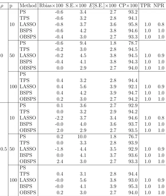
To assess the variable selection performance of BSPS, OBSPS, and LASSO meth-ods, we compute true positive rate (TPR) and true negative rate (TNR), where TPR is the proportion of the regression coefficients that are correctly identified as nonzero and TNR is the proportion of the regression coefficients that are correctly identified as zero. The coverage probabilities of each methods are computed by counting how of-ten the confidence intervals contain the true parameter values. In BSPS and LASSO, we present TPR and TNR for the response model. In OBSPS, we show TPR and TNR for the working model to select correlated covariates. The simulation results for models M1 and M2 are presented in Tables 1and 2, respectively.

Table 1shows the numerical results for M1. Overall, the proposed methods

per-form similarly between correlated covariates (ρ = 0.5) and independent covariates (ρ = 0). When dimension is low, specifically, when p=10, PS and TPS have similar performance in terms of bias and standard errors. TPS are more efficient than PS due to sparsity. LASSO and BSPS can select the true response model with large probabilities. However, LASSO and BSPS obtain larger standard errors than TPS due to additional model uncertainty under finite samples. Overall, BSPS outperforms LASSO in term of model consistency. OBSPS always provides the most efficient esti-mators by incorporating relevant auxiliary variables from the full sample. For small

p, all methods achieve approximately 95% coverage probabilities for corresponding confidence intervals or credible intervals for Bayesian models.

When p increases to 50 in M1, the PS estimator using all variables shows large

standard errors. Moreover, the average of the estimated standard errors for the PS estimator is much smaller than the true standard error of the PS estimator, which leads to biased interval estimation and low coverage probability. Note that TPS is the gold standard method, where we pretend that we know the truth. Thus, TPS is invariant for large p. BSPS performs better than LASSO for selecting the true response model. Therefore, the model uncertainty of BSPS and OBSPS are much smaller than LASSO. Table 1 shows that Monte Carlo standard error of LASSO is much larger than estimated standard error due to model uncertainty. However, the increased variances of BSPS and OBSPS are not as obvious as LASSO due to better model selection performance. In summary, BSPS obtains comparable estimator and inference with TPS. OBSPS is still most efficient relative to all other methods and it identifies the relevant covariates with probability one.

When pincreases to 100, PS fails to achieve convergence in solving score equation of φ. Thus, no numerical results are presented for PS. LASSO obtains low coverage probabilities, because of large model uncertainty. However, BSPS still works well and obtains similar performance with TPS. OBSPS outperforms by far all other methods. Table 2 presents the numerical results for M2, where the outcome model is

1can be made for the results of Table2. OBSPS can only correctly identifyxi4

with-out xi3, since xi3 is not correlated with y, even though the true outcome model has

x2

i3. Overall, OBSPS is the most efficient method. The model uncertainty of LASSO

keeps increasing as p increase, which leads to low coverage probabilities and biased estimation for standard errors. BSPS achieves comparable results with TPS.

6.2

Simulation study II

We also apply the Bayesian sparse propensity score method to the 2006 Korean Labor and Income Panel Survey (KLIPS) data. A breif description of the panel survey can be found at http://www.kli.re.kr/klips/en/about/introduce.jsp. In KLIPS data, there are 2,506 regular wage earners. The study variable y is the monthly income in 2006. The auxiliary variables (x) include the average monthly income in previous year and demographic variables. We grouped age into three levels: age < 35,35 ≤ age <

51,age ≥51.

In this simulation study, we use the KLIPS data as a finite population. The real-ized sample is then obtained from the population by Simple Random Sampling (SRS) with sample sizen = 200 independently. Since the KLIPS data are fully observed, we artificially create a nonresponse scheme by applying the missing mechanismRin (28). Note the two major differences here compared with the first simulation study. One is the mixed data types of the auxiliary variables. Another is the unknown outcome regression model. The simulation process is described in the following:

Step 1: Obtain 200 samples from the KLIPS data by SRS.

Step 2: Apply the response mechanism Rto the sample, so that the auxiliary variables are fully observed and the study variable y is subject to missingness.

Step 3: Apply the PS, LASSO, BSPS and OBSPS methods in simulation study I to the incomplete sample.

The true response function R is

P r(δi = 1 |xi, yi) =

exp(φ0+φ1xi9)

1 + exp(φ0+φ1xi9)

, (28)

where (φ0, φ1) = (3,−1), xi9 is average monthly income in the previous year, and the

response rate is approximately 70%. Suppose we are interested in the average monthly income θ=E(y). To fit the response model, we assume the response mechanism is

P r(δi = 1|xi, yi) = exp(xT i φ) 1 + exp(xT i φ) =:π(φ;xi),

which is known up to the parameterφ. Thus, the joint estimating equations are

Un(φ, θ) = n−1Pn i=1{δi−π(φ;xi)}xi n−1Pn i=1 δi π(φ;xi)(yi−θ). (29) The analysis result is summarized in Table 3.

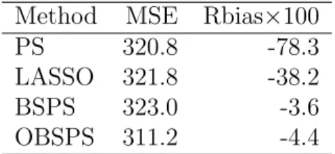
From Table 3, the mean square errors of all four methods are similar. However, the proposed optimal Bayesian sparse propensity score method (OBSPS) is most effi-cient, because OBSPS incorporates the relevant auxiliary variables in propensity score estimation. Due to large dimensions of auxiliary variables, the traditional propensity score (PS) estimation including all variables fails to provide a consistent variance es-timator, as explained in Theorem 1. The propensity score model using LASSO also highly underestimates the variance due to large model uncertainty. In summary, the proposed BSPS and OBSPS provide consistent variance estimators uniformly regard-less of the dimension of covariates.

7

Discussion

This paper presents a Bayesian approach to PS estimation using the Spike-and-Slab prior for the response propensity model. Through the proposed BSPS method, model selection consistency holds and the uncertainty in model selection is fully captured by the Bayesian framework. The efficiency of the PS estimation can be further improved by incorporating relevant auxiliary variables, the so-called optimal Bayesian sparse propensity score (OBSPS) method. The simulation study in Section6shows that the Bayesian approach provides valid frequentist coverage probabilities in finite samples.

Since the PS estimation is widely used in causal inference (Morgan and Winship,

2014; Hudgens and Halloran, 2008), applying the proposed methods to the sparse

Bayesian causal inference can be developed similarly. Also, our proposed method is developed under the assumption of MAR. Extension of our proposed method to nonignorable nonresponse is a topic for future research.

Table 1: Simulation results for M1: “Bias” is the bias of the point estimator for θ,

“S.E.” represents the standard error of the point estimator, “E[S.E.]” is the average of the estimated standard error, “CP” represents the coverage probability of the 95% confidence interval estimate.

ρ p Method Rbias×100 S.E.×100 E[S.E.]×100 CP×100 TPR NPR

0 10 PS -0.6 3.4 2.7 93.2 TPS -0.6 3.2 2.8 94.1 LASSO -0.8 3.7 3.6 95.8 1.0 0.8 BSPS -0.6 4.2 3.8 94.6 1.0 1.0 OBSPS -0.4 3.0 2.7 93.3 1.0 1.0 50 PS -0.6 9.4 1.8 78.7 TPS -0.2 3.0 2.8 94.5 LASSO -0.2 4.5 3.8 94.5 1.0 0.9 BSPS -0.4 4.1 3.8 94.3 1.0 1.0 OBSPS 0.0 2.9 2.7 94.0 1.0 1.0 100 PS TPS 0.4 3.2 2.8 94.4 LASSO 0.4 5.6 3.9 92.1 1.0 0.9 BSPS 0.4 4.2 3.9 94.7 1.0 1.0 OBSPS 0.2 3.0 2.7 94.2 1.0 1.0 0.5 10 PS 0.1 3.6 2.7 92.9 TPS 0.0 3.2 2.9 94.2 LASSO -2.2 3.7 3.4 94.6 1.0 0.8 BSPS -0.0 4.0 3.6 93.7 1.0 1.0 OBSPS 2.0 2.9 2.7 93.5 1.0 1.0 50 PS 0.2 10.0 1.8 76.7 TPS 0.0 3.3 2.8 93.9 LASSO -1.8 4.4 3.5 92.9 1.0 0.9 BSPS 0.0 4.1 3.7 93.6 1.0 1.0 OBSPS 2.4 3.0 2.7 93.3 1.0 1.0 100 PS TPS 0.4 3.1 2.8 94.4 LASSO -0.0 5.6 3.8 93.0 1.0 0.9 BSPS -0.0 4.1 3.9 95.3 1.0 1.0 OBSPS 0.2 3.0 2.7 94.0 1.0 1.0

Table 2: Simulation results forM2: “RBias” is the relative bias of the point estimator

for θ, “S.E.” represents the standard error of the point estimator, “E[S.E.]” is the average of the estimated standard error, “CP” represents the coverage probability of the 95% confidence interval estimate

.

ρ p Method Rbias×100 S.E.×100 E[S.E.]×100 CP×100 TPR NPR

0 10 PS 0.2 3.7 3.1 92.7 TPS 0.4 4.5 4.2 94.2 LASSO 0.4 4.0 4.1 95.1 1.0 0.8 BSPS 0.4 4.4 4.2 94.0 1.0 1.0 OBSPS 0.2 3.4 3.1 93.5 1.0 1.0 50 PS 0.0 9.5 2.1 80.2 TPS 0.2 4.5 4.2 94.8 LASSO 0.2 5.0 4.2 94.2 1.0 0.9 BSPS 0.0 4.4 4.2 95.0 1.0 1.0 OBSPS -0.0 3.2 3.1 94.3 1.0 1.0 100 PS TPS -0.2 4.7 4.2 93.9 LASSO -0.2 6.3 4.2 91.9 1.0 0.9 BSPS -0.2 4.6 4.2 93.6 1.0 1.0 OBSPS -0.4 3.4 3.1 93.5 1.0 1.0 0.5 10 PS 0.8 3.7 3.1 92.7 TPS 0.8 4.2 3.9 93.7 LASSO -0.8 3.9 3.8 94.3 1.0 0.8 BSPS 0.8 4.3 4.0 93.9 1.0 1.0 OBSPS 1.0 3.4 3.1 93.4 1.0 1.0 50 PS -0.4 7.3 2.1 80.9 TPS -0.4 4.2 3.9 94.6 LASSO -2.0 4.5 4.0 94.2 1.0 0.9 BSPS -0.4 4.3 4.0 94.7 1.0 1.0 OBSPS -0.2 3.3 3.1 94.1 1.0 1.0 100 PS TPS -0.2 4.2 3.9 94.3 LASSO -1.6 5.3 4.0 93.0 1.0 0.9 BSPS -0.0 4.2 4.0 94.7 1.0 1.0 OBSPS -0.0 3.3 3.1 93.9 1.0 1.0

Table 3: Simulation result for the 2006 Korean Labor and Income Panel Survey. “MSE” is the mean squared error. “Rbias” represents the relative bias of the variance estimator.

Method MSE Rbias×100 PS 320.8 -78.3 LASSO 321.8 -38.2 BSPS 323.0 -3.6 OBSPS 311.2 -4.4

Appendices

In these appendices, we present the technical derivations and proofs for all stated theorems in this paper.

A

Computational details

To generate φ(t+1) from (18), the computation using the Metropolis-Hastings al-gorithm (Chib and Greenberg, 1995) can be quite heavy. Thus, instead of using the likelihood function of φ directly, we propose to use the Laplace approxima-tion method. To discuss the approximaapproxima-tion of (18), let ˆφ(t+1) _{be the maximizer of}

L1(φ|data)p(φ|z(t+1)). From the Spike-and-Slab prior in (9),p(φ |z(t+1)) is a

Gaus-sian distribution with mean 0 and variance V_z(t+1) = Diag ν_z(t+1) 1 , ν_z(t+1) 2 , . . . , ν_z(t+1) p , where ν_z(t+1) j =ν1z (t+1) j +ν0(1−z (t+1)

j ). Thus, maximizingL1(φ|data)p(φ|z(t+1)) is

equivalent to solving Sn(φ)−V_z−(t1+1)φ = 0. (30) Denote ˆ Vφ= nIφ+V_z−(t1+1) −1 , (31)

where Iφ is the negative fisher information matrix of φ defined as

Iφ=E ∂2_logf(δ i |xi, φ) ∂φ∂φT .

Note that Vφ is always positive definite. Using second oder Taylor expansion, the

Laplace approximation is L1(φ|data)p(φ |z(t+1))∼= L1( ˆφ(t+1) |data)p( ˆφ(t+1) |z(t+1)) ×exp −1 2(φ− ˆ φ(t+1))TVˆ_ˆ−1 φ(t+1)(φ−φˆ (t+1)₎ .

Therefore, generatingφ(t+1)from (18) is approximately equivalent to generatingφ(t+1)

fromN( ˆφ(t+1)_,Vˆ ˆ

φ(t+1)), where ˆV_φˆ(t+1) is a consistent estimator with plugged in ˆI_φˆ(t+1).

For Step 2b, note that, under some regularity conditions, we can establish that

n−1/2 Sn(φz(t+1)) UP S(θ, φz(t+1)) φ_z(t+1), θ L −→N 0,Σ(t+1) . (32)

Correspondingly, Σ(t+1) _{= Σ}(t+1)_(φ z(t+1), θ) can be decomposed as Σ(t+1) = Σ (t+1) 11 Σ (t+1) 12 Σ(₂₁t+1) Σ(₂₂t+1) ! .

Thus, the asymptotic distribution in (32) implies that√nUP S(θ, φz(t+1))|S_n(φ_z(t+1)), θ, φ(t+1) z(t+1)

goes to a normal distribution

N Σ(₂₁t+1)Σ(₁₁t+1) −1 Sn(φ (t+1) z(t+1)),Σ (t+1) 22·1 , where Σ(t+1) _{= Σ}(t+1)_(φ(t+1) z(t+1), θ) and Σ (t+1) 22·1 = Σ (t+1) 22 −Σ (t+1) 21 Σ(₁₁t+1) −1 Σ(₁₂t+1). There-fore, g2 n UP S(θ, φz(t+1))|S_n(φ_z(t+1)), θ, φ (t+1) z(t+1) o

is a normal density function.

To establish consistency, we assume the following condition to avoid unnecessary details :

(A5) The ˆVφ in (31) satisfies ˆVφ=Vφ{1 +op(1)}.

B

Implementation of the

P-step

Given u(t+1)_{, σ}2,(t)

e , generate β(t+1) from a multivariate Gaussian distribution with

mean µ∗ and variance V∗, where

V∗ = V_u−(t1+1) + Pn i=1δixix T i σe2,(t) −1 , µ∗ = V−1 u(t+1) + Pn i=1δixix T i σe2,(t) −1P i=1δixiyi σe2,(t) , (33) and V_u(t+1) = Diag n γ_u(t+1) 1 ,· · · , γ_u(t+1) p o . Then, givenβ(t+1)_{, σ}2,(t+1) e is generated from

a inverse gamma distribution with parameters (c∗₁, c∗₂), where

c∗₁ =c1+ r 2, c∗₂ =c2+ 1 2 n X i=1 δi(yi−xiTβ(t+1))2. (34)

C

Proof of Theorem

1

Without loss of generality, we assume

E(XXT ) =   E(X1X1T) 0 0 0 E(X2X2T) 0 0 0 E(X3X3T)   (35)

to simplify the proof.

Assume ˆη = ( ˆφ,θˆ) is the solution of

Un(η) = n−1Pn i=1S(φ;xi, δ) n−1Pn i=1δiπ −1_(φ;x i)U(θ;xi, yi) ,

where π(φ;xi) = G(xTiφ). Thus, we can derive the score function ofφ as

S(φ;xi, δi) = δi G(xT iφ) − 1−δi 1−G(xT iφ) G0(xT iφ)xi,

where G0(·) is the first order derivative of G(·).

We first consider that p3 = O(1). Applying the Taylor expansion to the joint

estimating equations, we have

Un(ˆη) =Un(η0) +E ( ∂Un(η) ∂ηT η=η0 ) (ˆη−η0) +Op(kηˆ−η0k2).

If p3 =O(1), we can ignore the smaller term and obtain

ˆ η−η0 =− " E ( ∂Un(η) ∂ηT η=η0 )#−1 Un(η0).

Then, the variance is asymptotically equal to var (ˆη−η0) = " E ( ∂Un(η) ∂ηT η=η0 )#−1 var{Un(η0)} " E ( ∂Un(η) ∂ηT η=η0 )#−1,T . (36) Now, let us compute the variance in (36). First, we can show that

E ( ∂Un(η) ∂ηT η=η0 ) = A 0 C D , where A =−EhG−1(XT φ0) +{1−G(XTφ0)} −1i G0(XT φ0)G0(XTφ0)XXT , C=−EnG−1(XT φ0)G 0 (XT φ0)U(θ0;X, Y)XT o , D=E ∂U(θ0;X, Y) ∂θ .

Under the true model assumption, we have G(XT_φ

0) =G(X1Tφ0,1) =G0(X1), where

φ0 = (φ0,1,0,0). Moreover, we can decomposeA as

A=   A1 0 0 0 A2 0 0 0 A3  , (37)

where A1 =−E G−₀1(X1) +{1−G0(X1)} −1 G0₀(X1)G00(X1)X1X1T , A2 =−E G−₀1(X1) +{1−G0(X1)} −1 G0₀(X1)G00(X1) E(X2X2T), A3 =−E G−₀1(X1) +{1−G0(X1)} −1 G0₀(X1)G00(X1) E(X3X3T).

Similarly, we can show that

C =−EnG−₀1(X1)G 0 0(X1)U(θ0;X, Y)X1T o ,−EnG−₀1(X1)G 0 0(X1)U(θ0;X, Y)X2T o ,0 =: (C1, C2,0).

Then, we derive the variance of Un(η0) as

var{Un(η0)} =E Un(η0)UnT(η0) =n−1 −A −CT −C E{U2_(θ 0;X, Y)} (38) To compute the variance of ˆη, we apply block matrix inverse formula to

E ( ∂Un(η) ∂ηT η=η0 ) . That is A 0 C D −1 = A−1 ₀ −D−1_CA−1 _D−1 .

Finally, we can obtain that var (ˆη−η0) =n−1 A−1 ₀ −D−1CA−1 D−1 −A −CT −C E{U2(θ0;X, Y)} A−1 _−A−1_CT_D−1 0 D−1 =n−1 −A−1 ₀ 0 D−1_E{U2_(θ 0;X, Y)}D−1+D−1CA−1C−1D−1 =: Σ. Therefore, we have var(ˆθP S) = n−1E ∂U(θ0;X, Y) ∂θ EU2(θ0;X, Y) E ∂U(θ0;X, Y) ∂θ +E ∂U(θ0;X, Y) ∂θ C1A−11C T 1 +C2A−21C T 2 E ∂U(θ0;X, Y) ∂θ .

Since A1, A2 is negative definite, E ∂U(θ0;X, Y) ∂θ C1A−11C T 1 E ∂U(θ0;X, Y) ∂θ ≤0 E ∂U(θ0;X, Y) ∂θ C2A−21C T 2 E ∂U(θ0;X, Y) ∂θ ≤0.

Therefore, the PS estimator using the true response probability is less efficient than the PS estimator using the true response model with estimated response probability. Moreover, the PS estimator using estimated response probability in the true response model is less efficient than the PS estimator using estimated response probability including X2. This completes the proof for the last part of Theorem1.

Then, we considerp3 =p3(n) case. Under this case,Op(kηˆ−η0k2) is not negligible.

We expand Un(ˆη) to the second order term in Taylor expansion. That is

Un(ˆη) =Un(η0) +E ( ∂Un(η) ∂ηT η=η0 ) (ˆη−η0) +R+Op(kηˆ−η0k3), whereR= (R1,· · · , Rp+1),Rj = 1₂Pp_j=1(ˆη−η0)THj(ˆη−η0) andHj =E n ∂2_U n(η)/∂ηT∂ηj|_η=η0 o . Thus, E(ˆη−η0)∼=− " E ( ∂Un(η) ∂ηT η=η0 )#−1 E(R). (39) Assume E ( ∂Un(η) ∂ηT _η=η 0 ) =O(1).

Moreover, assume Hj =O(1). Then we have

E(Rj) =O[E{(ˆη−η0)THj(ˆη−η0)}]

=O(Trace [E{Hj(ˆη−η0)(ˆη−η0)T}])

=O(Trace [E{(ˆη−η0)(ˆη−η0)

T

}])

=On−1Trace(A₁−1) + Trace(A−₂1) + Trace(A−₃1) =Op3 n , which leads to µ=EθˆP S−θ0 =O(p3/n) = O(p/n).

Similarly, var (Rj) = O[var{(ˆη−η0)THj(ˆη−η0)}] =O{Trace (HjΣHjΣ)}+O µTHjΣHjµ =O{Trace(ΣΣ)}+O(µTΣµ) =On−2Trace(A−1) +O p2 3 n3 =O p₃ n2 +O p2 3 n3 . (40)

Let ˆηj = ˆθP S and we have

varθˆP S−θ0

=O(1/n) +Op3n−2(1 +p3/n) .

We complete the proof for Theorem1.

D

Proof of Theorem

2

Let V = n−1_I−1

φ0 in (31). Our proof can be summarized as follows: First, we show

that ˜ p(zo|data) p →1, (41) as n→ ∞, where ˜ p(zo|data) = R ψ( ˆφ|φ, V)p(φ|zo)p(zo)dφ R R ψ( ˆφ|φ, V)p(φ|z)p(z)dφdz,

ψ(· | φ, V) is the normal density function with mean φ and variance V, and ˆφ is the maximizer of L1(φ |data).

Second, we show that

|p˜(zo|data)−pg(zo|data)| p

→0, (42)

as n→ ∞. Note that

|p˜(zo|data)−pg(zo|data)| ≥ ||p˜(zo|data)−1| − |pg(zo|data)−1||.

Finally, by (41) and (42), we have that

pg(zo|data) p

→1,

Proof of Claim (41)

Under (A4), sinceπ(z)∝1, ˜p(zo|data) reduces to

˜ p(zo|data) = R ψ( ˆφ|φ, V)p(φ|zo)dφ P z∈{0,1}p R ψ( ˆφ|φ, V)p(φ|z)dφ := f( ˆφ|zo) P z∈{0,1}pf( ˆφ|z) = 1 1 +P z6=zo f( ˆφ|z) f( ˆφ|zo) ,

where f( ˆφ|z) = R ψ( ˆφ|φ, V)p(φ|z)dφ. Our proof can be done by showing that

X z6=zo f( ˆφ|z) f( ˆφ|zo) p →0, (43) as n → ∞. Since Σ = I−_φ1

0 is symmetric and positive definite, by spectral

decompo-sition, Σ can be factorized as Σ = QΛQ−1, where Λ is the diagonal matrix whose diagonal elements are the eigenvalues of Σ and each column of Q is the eigenvec-tor of Σ. Since V = n−1_{Σ, we have V = Q(n}−1_Λ)Q−1_{. Let λ}

n,min = n−1λmin and

λn,max =n−1λmax, whereλmin and λmaxindicate the smallest and the largest diagonal

elements of Λ, respectively. Note that λ−_n,1_minI−V−1 _{and V}−1_−λ

n,maxI are positive

semidefinite due to the fact that

λ_n,−1_minI−V−1 =Q λ_n,−1_minI−nΛ−1Q−1, V−1−λ−_n,1_maxI =Q nΛ−1−λ−_n,1_maxIQ−1.

This implies that

λ−_n,1_maxwT

w≤wT

V−1w≤λ−_n,1_minwT

w, (44)

for any w. Recall that

ψ( ˆφ|φ, V) =cexp −1 2 ˆ φ−φ T V−1φˆ−φ ,

where cdenotes the normalizing constant. From (44), we have

ψ( ˆφ|φ, V)≥cexp ( − p X j=1 1 2λn,min ˆ φj−φj 2 ) , (45) ψ( ˆφ|φ, V)≤cexp ( − p X j=1 1 2λn,max ˆ φj−φj 2 ) . (46)

Using (45), we construct a lower bound of f( ˆφ|z) =R ψ( ˆφ|φ, V)p(φ|z)dφ as f( ˆφ|z) ≥ c p Y j=1 2πνzj −1/2 Z exp − 1 2λn,min ˆ φj−φj 2 − 1 2νzj φ2_j dφj = c2 p Y j=1 λn,min λn,min+νzj 1/2 exp ( − ˆ φ2 j 2 λn,min+νzj ) ≡Lf(z).

Similarly, using (46), we construct an upper bound of f( ˆφ|z) as

f( ˆφ|z) ≤ c3 p Y j=1 λn,max λn,max+νzj 1/2 exp ( − ˆ φ2_j 2 λn,max+νzj ) ≡Uf(z). Hence, we have f( ˆφ|z) f( ˆφ|zo) ≤ Uf(z) Lf(zo) . (47) We now claim Uf(z) Lf(zo) p

→0 as n →0 for anyz 6=zo. Define

Hn(zj, zo,j) =

λn,max(λn,min+νzo,j)

λn,min(λn,max+νzj) 1/2 exp ( − ˆ φ2 j 2(λn,max+νzj) + ˆ φ2 j 2(λn,min+νzo,j) ) .

Suppose zo,j = 0. Then we have that ˆφ2j = Op(n−1) from Theorem 1. Recall that

from (A4),ν0 =o(n−1). If zj = 0, then Hn(0,0) = λn,max(λn,min+ν0) λn,min(λn,max+ν0) 1/2 exp ( − ˆ φ2 j 2(λn,max+ν0) + ˆ φ2 j 2(λn,min+ν0) ) = O(n−2_{) +o(n}−2₎ O(n−2_{) +o(n}−2₎ 1/2 exp − Op(n −1₎ O(n−1_{) +o(n}−1₎ + Op(n−1) O(n−1_{) +o(n}−1₎ .

This implies that Hn(0,0) = 1 in probability. From (A4), we have ν1 = O(n). If

zj = 1, then Hn(1,0) = λn,max(λn,min+ν0) λn,min(λn,max+ν1) 1/2 exp ( − ˆ φ2_j 2(λn,max+ν1) + ˆ φ2_j 2(λn,min+ν0) ) = O(n−2_{) +o(n}−2₎ O(n−2_{) +O(1)} 1/2 exp − Op(n −1₎ 2{O(n−1_{) +O(n)}}+ Op(n−1) 2{O(n−1_{) +o(n}−1_)} .

If zj = 0, then Hn(0,1) = λn,max(λn,min+ν1) λn,min(λn,max+ν0) 1/2 exp ( − ˆ φ2_j 2(λn,max+ν0) + ˆ φ2_j 2(λn,min+ν1) ) = O(n−2_{) +O(1)} O(n−2_{) +o(n}−2₎ 1/2 exp − Op(1) 2{O(n−1_{) +o(n}−1_)}+ Op(1) 2{O(n−1_{) +O(n)}} =O(n) exp{−Op(n)}.

This implies that Hn(0,1) =Op{exp(−n)}. When zj = 1, we have

Hn(1,1) = λn,max(λn,min+ν1) λn,min(λn,max+ν1) 1/2 exp ( − ˆ φ2_j 2(λn,max+ν1) + ˆ φ2_j 2(λn,min+ν1) ) = O(n−2_{) +O(1)} O(n−2_{) +O(1)} 1/2 exp − Op(1) 2{O(n−1_{) +O(n)}} + Op(1) 2{O(n−1_{) +O(n)}} .

This implies that Hn(1,1) =Op(1). Note that

Uf(z) Lf(zo) ∝ p Y j=1 Hn(zj, zo,j).

If z6=zo, then Qp_j=1Hn(zj, zo,j) must include at least one of Hn(1,0) or Hn(0,1).

Note that P z6=zo f( ˆφ|z) f( ˆφ|zo) ≤c4 X z6=zo Uf(z) Lf(zo) ≤c4 X j1≤p1,j2≤p−p1,j3≤p1,j4≤n−p1,j1+j2+j3+j4=p,j2+j3>0 Hj1 n (1,1)H j2 n(1,0)H j3 n(0,1)H j4 n(0,0). ≤c4Hnp1(1,1) X j2≤p−p1,j3≤p1,j4≤n−p1,j2+j3+j4=p,j2+j3>0 Hj2 n (1,0)Hnj3(0,1)Hnj4(0,0).

Since we have shown that Hn(1,1) = Hn(0,0) = Op(1), Hn(1,0) = Op(n−1) and

Hn(0,1) = Op(exp(−n)), we can show that Hnp1(1,1) =Op(1) and X j2≤p−p1,j3≤p1,j4≤n−p1,j2+j3+j4=p,j2+j3>0 Hj2 n(1,0)H j3 n(0,1)H j4 n(0,0) ≤ X j2≤p−p1,j4≤n−p1,j2+j4=p,j2>0 Hj2 n(1,0)H j4 n(0,0). ≤ {Hn(0,0) +Hn(1,0)} p −H_np(0,0) =1 +Op(n−1) p −1.

We know that

lim

n∞(1 +an

−1₎n _=ea_,

for any a >0. Thus,

1 +Op(n−1) p

−

→1 (48)

in probability, if p=o(n). This implies that

X z6=zo f( ˆφ|z) f( ˆφ|zo) − →0,

in probability. This completes our proof.

Proof of Claim (42)

First, we show that

ψ( ˆφ|φ,Vˆ) =ψ( ˆφ|φ, V){1 +op(1)}, where ˆV =n−1Σ. In (ˆ A5), we have ˆ Σ = Σ{1 +op(1)}. Under Σ>0, |Σˆ|−1/2 =|Σ|−1/2{1 +op(1)}. Therefore, we have ψ( ˆφ|φ,Vˆ) = 1 (2π)p2|V| 1 2 exp −1 2 ˆ φ−φ T V−1φˆ−φ{1 +op(1)} {1 +op(1)}.

To complete the proof, we need to show that exp −1 2 ˆ φ−φ T V−1φˆ−φop(1) =Op(1). (49) From (44), we have n 2λmax kφˆ−φk2 ≤ 1 2 ˆ φ−φ T V−1 ˆ φ−φ ≤ n 2λmin kφˆ−φk2,

where λmin and λmax are the smallest and the largest eigenvalues of Σ, respectively.

From (40) and p3 = o(n), we have kφˆ−φk2 = Op(n−1). This implies our claim in

(49). Note that, ln(φ) =ln( ˆφ) + ∂ln(φ) ∂φT φ= ˆφ (φ−φˆ) + 1 2(φ− ˆ φ)T ∂ 2_l n(φ) ∂φ∂φT φ= ˆφ ! (φ−φˆ) +op 1 n ,

which implies that

L1(φ |data) =ψ( ˆφ|φ,Vˆ)(1 +op(1)) =ψ( ˆφ |φ, V)(1 +op(1)). Note that, ˜ p(zo|data) = R ψ( ˆφ|φ, V)p(φ|zo)p(zo)dφ R R ψ( ˆφ|φ, V)p(φ|z)p(z)dφdz, and pg(zo|data) = R L1(φ|data)p(φ|zo)p(zo)dφ R R L1(φ|data)p(φ|z)p(z)dφdz .

Since we have shown thatL1(φ |data) =ψ( ˆφ|φ, V){1 +op(1)}, we thus obtain

|p˜(zo|data)−pg(zo|data)| p

→0,

References

M. A. Beaumont, W. Zhang, and D. J. Balding. Approximate Bayesian computation in population genetics. Genetics, 162(4):2025–2035, 2002.

G. Casella and E. I. George. Explaining the Gibbs sampler. The American Statisti-cian, 46(3):167–174, 1992.

G. Casella, F. J. Giron, M. L. Martinez, and E. Moren. Consistency of Bayesian procedures for variable selection. The Annals of Statistics, 37(3):1207–1228, 2009. J. Chen and Z. Chen. Extended Bayesian information criteria for model selection

with large model spaces. Biometrika, 95(3):759–771, 2008.

S. Chib and E. Greenberg. Understanding the Metropolis-Hastings algorithm. The

American Statistician, 49(4):327–335, 1995.

J. Fan and R. Li. Variable selection via nonconcave penalized likelihood and its Oracle properties. Journal of the American Statistical Association, 96:1348–1360, 2001. W. D. Flanders and S. Greenland. Analytic methods for two-stage case-control studies

and other stratified designs. Statistics in Medicine, 10(5):739–747, 1991.

J. Friedman, T. Hastie, and R. Tibshirani. glmnet: Lasso and elastic-net regularized generalized linear models. R package version, 1(4), 2009.

E. I. George and R. E. McCulloch. Variable selection via Gibbs sampling. Journal of

the American Statistical Association, 88(423):881–889, 1993.

E. I. George and R. E. McCulloch. Approaches for Bayesian variable selection.

Sta-tistica sinica, pages 339–373, 1997.

M. G. Hudgens and M. E. Halloran. Toward causal inference with interference.

Jour-nal of the American Statistical Association, 103(482):832–842, 2008.

J. K. Kim and J. J. Kim. Nonresponse weighting adjustment using estimated response probability. Canadian Journal of Statistics, 35(4):501–514, 2007.

J. K. Kim and J. Shao. Statistical Methods for Handling Incomplete Data. CRC Press, 2013.

M. Kyung, J. Gilly, M. Ghosh, and G. Casella. Penalized Regression, Standard Errors, and Bayesian Lassos. Bayesian Analysis, 5:369–412, 2010.

J. D. Lee, D. L. Sun, Y. Sun, J. E. Taylor, et al. Exact post-selection inference, with application to the LASSO. The Annals of Statistics, 44(3):907–927, 2016.

R. J. Little and D. B. Rubin. Statistical Analysis with Missing Data. John Wiley & Sons, 2002.

T. J. Mitchell and J. J. Beauchamp. Bayesian variable selection in linear regression.

Journal of the American Statistical Association, 83(404):1023–1032, 1988.

S. L. Morgan and C. Winship. Counterfactuals and Causal Inference. Cambridge University Press, 2014.

N. N. Narisetty, X. He, et al. Bayesian variable selection with shrinking and diffusing priors. The Annals of Statistics, 42(2):789–817, 2014.

M. C. Paik. The generalized estimating equation approach when data are not missing completely at random. Journal of the American Statistical Association, 92(440): 1320–1329, 1997.

T. Park and G. Casella. The Bayesian Lasso. Journal of the American Statistical

Association, 103:681–686, 2008.

J. M. Robins, A. Rotnitzky, and L. P. Zhao. Estimation of regression coefficients when some regressors are not always observed. Journal of the American statistical

Association, 89(427):846–866, 1994.

J. M. Robins, A. Rotnitzky, and L. P. Zhao. Analysis of semiparametric regression models for repeated outcomes in the presence of missing data. Journal of the

P. R. Rosenbaum. Model-based direct adjustment.Journal of the American Statistical

Association, 82(398):387–394, 1987.

D. B. Rubin. Inference and missing data. Biometrika, 63(3):581–592, 1976.

H. Sang and J. K. Kim. An approximate Bayesian inference on propensity score estimation under nonresponse. Submitted., 2018.

M. J. Silvapulle. On the existence of maximum likelihood estimators for the binomial response models.Journal of the Royal Statistical Society. Series B (Methodological), 43(3):310–313, 1981.

S. Soubeyrand and E. Haon-Lasportes. Weak convergence of posteriors conditional on maximum pseudo-likelihood estimates and implications in ABC. Statistics & Probability Letters, 107:84–92, 2015.

M. A. Tanner and W. H. Wong. The calculation of posterior distributions by data augmentation. Journal of the American statistical Association, 82(398):528–540, 1987.

R. Tibshirani. Regression Shrinkage and Selection via the Lasso. Journal of the Royal

Statistical Society, Series B, 58:267–288, 1996.

R. J. Tibshirani, J. Taylor, R. Lockhart, and R. Tibshirani. Exact post-selection inference for sequential regression procedures. Journal of the American Statistical

Association, 111(514):600–620, 2016.

G. C. Wei and M. A. Tanner. A Monte Carlo implementation of the EM algorithm and the poor man’s data augmentation algorithms. Journal of the American statistical

Association, 85(411):699–704, 1990.

M. Zhou and J. K. Kim. An efficient method of estimation for longitudinal surveys with monotone missing data. Biometrika, 99(3):631–648, 2012.

H. Zou. The Adaptive Lasso and Its Oracle Properties. Journal of the American

H. Zou and T. Hastie. Regularization and variable selection via the elastic net.Journal