Second order accurate variance estimation in poststratified two-stage sampling

(1)

A Dissertation by

KYONG RYUN KIM

Submitted to the Office of Graduate Studies of Texas A&M University

in partial fulfillment of the requirements for the degree of DOCTOR OF PHILOSOPHY

May 2006

(2)

A Dissertation by

KYONG RYUN KIM

Submitted to the Office of Graduate Studies of Texas A&M University

in partial fulfillment of the requirements for the degree of DOCTOR OF PHILOSOPHY

Approved by:

Chair of Committee, Suojin Wang Committee Members, Bani Mallick

Johan Lim Lihong Wang Head of Department, Simon J. Sheather

May 2006

(3)

ABSTRACT

Second Order Accurate Variance Estimation in Poststratified Two-stage Sampling. (May 2006)

Kyong Ryun Kim, B.S., Sungkyukwan University, Korea; B.S., Michigan State University;

M.S., Michigan State University

Chair of Advisory Committee: Dr. Suojin Wang

We proposed new variance estimators for the poststratified estimator of the popula-tion total in two-stage sampling. The linearizapopula-tion or Taylor series variance estimator and the jackknife linearization variance estimator are popular for the poststratified estimator. The jackknife linearization variance estimator utilizes the ratio, ˆRc, which

balances the weights for the poststrata while the linearization or Taylor series esti-mator does not. The jackknife linearization variance estiesti-mator is equivalent to Rao’s (1985) adjusted variance estimator. Our proposed estimator makes use of the ratio,

ˆ

Rc, in a different shape which is naturally derived from the process of expanding

to the second-order Taylor series linearization, while the standard linearization vari-ance estimator is only expanded to the first-order. We investigated the properties and performance of the linearization variance estimator, the jackknife linearization estimator, the proposed variance estimator and its modified version analytically and through simulation study. The simulation study was carried out on both artificially generated data and real data. The result showed that the second order accurate variance estimator and its modified version could be very good candidates for the variance estimation of poststratified estimator of population total.

(4)

(5)

ACKNOWLEDGEMENTS

I would like to express special thanks to my wife, Sungeun. Without her guidance and support this dissertation would not have existed. Her kindness and encouragement made the entire journey of this research very smooth and delightful. I am also grateful for Dr. Suojin Wang, Bani Mallick, Johan Lim, and Lihong Wang as committee members. Their critical reading and helpful comments have greatly improved the dissertation.

I thank my parents and my brother, Kyunghoon. I also thank my parents-in-law, sister-in-parents-in-law, Hyeun, and brother-in-parents-in-law, Ikro. I also thank my friends in College Station, Sukho Lee and Hyejin Shin, and Deukwoo Kwon, in Washington D.C., who helped and encouraged me in many ways.

(6)

TABLE OF CONTENTS Page ABSTRACT . . . iii DEDICATION . . . iv ACKNOWLEDGEMENTS . . . v TABLE OF CONTENTS . . . vi

LIST OF FIGURES . . . viii

LIST OF TABLES . . . x CHAPTER I INTRODUCTION . . . 1 II SAMPLING DESIGN . . . 3 2.1 Survey Sampling . . . 3 2.2 Probability Sampling . . . 4 2.3 Inclusion Probability . . . 5 2.4 Horvitz-Thompson Estimator . . . 6

III POINT ESTIMATION IN FINITE POPULATION . . . 8

3.1 Calibration Estimation . . . 8

3.2 Auxiliary Variable . . . 9

3.3 Generalized Regression Estimator . . . 10

3.4 Raking . . . 12

IV STRATIFICATION AND CLUSTERING . . . 17

4.1 Stratified Sampling . . . 17

4.2 Cluster Sampling . . . 19

4.3 Two-stage Sampling . . . 21

V POSTSTRATIFIED POINT ESTIMATOR . . . 24

5.1 Population Total . . . 24

5.2 Poststratified Estimator . . . 25

(7)

CHAPTER Page

6.1 Variance Estimator in Estimating Population Total . . . . 29

6.2 The Jackknife Method . . . 29

6.3 Linearization Variance Estimator . . . 33

6.4 Jackknife Linearization Variance Estimator . . . 34

6.5 New Proposed Linearization Variance Estimator . . . 37

VII SIMULATION STUDY I . . . 42

VIII SIMULATION STUDY II . . . 61

8.1 Homogeneous vs Nonhomogeneous . . . 61

IX CONCLUDING REMARKS . . . 73

REFERENCES . . . 74

(8)

LIST OF FIGURES

FIGURE Page

1 Poststratification . . . 26 2 Point estimates of population total on 1,000 samples from the

simulated population under one-stage cluster sampling, n= 4 . . . . 48 3 Point estimates of population total on 1,000 samples from the

simulated population under two-stage cluster sampling, selecting

eight clusters per stratum and m = 6 units in each cluster . . . 52 7 Point estimates of population total on 1,000 samples from the

eight clusters per stratum and m = 18 units in each cluster . . . 55 10 Variance estimates based on 1,000 samples from the simulated

population under two-stage cluster sampling, selecting eight

clus-ters per stratum and m= 6 units in each cluster . . . 56 11 Variance estimates based on 1,000 samples from the simulated

(9)

FIGURE Page 12 Variance estimates based on 1,000 samples from the simulated

clus-ters per stratum and m= 14 units in each cluster . . . 58 13 Variance estimates based on 1,000 samples from the simulated

clus-ters per stratum and m= 18 units in each cluster . . . 59 14 Relative mse, P1000_i=1 (vi−vE

vE )

2_/1,_{000, of variance estimators in}

one-stage and two-one-stage where n = number of sampling cluster per stratum, m = number of units within each sampling cluster: in order of standard variance estimator(1), jackknife linearization es-timator(2), second order linearization estimator(3) and its adjuster

version(4) . . . 60 15 Point estimates of population total on 1,000 samples from the

homogeneous simulated population when A configuration . . . 65 16 Point estimates of population total on 1,000 samples from the

homogeneous simulated population when B configuration . . . 66 17 Point estimates of population total on 1,000 samples from the

heterogeneous simulated population when C configuration . . . 67 18 Point estimates of population total on 1,000 samples from the

heterogeneous simulated population when D configuration . . . 68 19 Variance estimates of population total on 1,000 samples from the

homogeneous simulated population when A configuration . . . 69 20 Variance estimates of population total on 1,000 samples from the

homogeneous simulated population when B configuration . . . 70 21 Variance estimates of population total on 1,000 samples from the

heterogeneous simulated population when C configuration . . . 71 22 Variance estimates of population total on 1,000 samples from the

(10)

LIST OF TABLES

TABLE Page

1 2_×2 problem with additional unknown row and column . . . 14

2 Distribution of unknowns to the known marginals . . . 14

3 First step in raking with rows . . . 15

4 First step in raking with columns . . . 15

5 Second step in raking with rows & columns . . . 15

6 Point estimators at one-stage on the simulated population . . . 45

7 Point estimators at two-stage on the simulated population . . . 45

8 Variance estimators at one-stage on the simulated population . . . 46

9 Variance estimators at two-stage on the simulated population . . . . 46

10 Point estimators at two-stage on the third grade population . . . 47

11 Variance estimators at two-stage on the third grade population, n1 = 11, n2= 16, n3 = 10, n4 = 23 . . . 47

12 Case A in homogeneous population . . . 63

13 Case B in homogeneous population . . . 63

14 Case C in nonhomogeneous population . . . 64

(11)

CHAPTER I

INTRODUCTION

Poststratified estimation of population total is one of popular methods in point esti-mation used in survey sampling. Poststratification can improve accuracy of estimate by using demographic information of population level that are already known. How-ever, poststratum identifiers of indivisual units are not usually available at the design stage. Therefore, the number of sampling units from each poststratum is random. That implies that can be made both unconditionally and conditionally (Yung and Rao 1996). As for the variance estimation, previous research has adopted two prin-cipal approaches, linearization methods and resampling methods. A linearization method involves the analytic calculations of linearizing procedure for a new variable. An advantage of the linearization method is that it is applicable to general sampling design, but it requires the derivation of a separate standard error formula and can be tedious, especially for nonlinear statistics. For example, when estimating ratio or regression coefficients, linearization method is very common (see Rao 1988). Re-sampling procedures, such as the jackknife, balanced repeated replicaton (BRR) and bootstrap, reuse the procedure for computing the point estimator repeatedly, using computing power to reduce the theoretical work. The jackknife variance estimator is one of the most frequently used method in practice. By linearizing the jackknife variance estimator, jackknife linearization variance estimator can be obtained which is identical to Rao’s (1985) variance estimator when estimating the variance of the

(12)

poststratified estimator. Valliant (1993) studied the standard linearization variance estimator, the balanced repeated replication, and the jackknife linearization variance estimator to determine if they estimate the conditional variance of the poststratified estimator of a finite population total under a super population model. Yung and Rao (1996) studied the standard linearization variance estimator, the jackknife and the jackknife linearization variance estimators for both the poststratified estimator and the regression estimator. Their simulation study suggested that the three variance estimators perform similarly, while an incorrect jackknife procedure which does not recalculate the regression weights each time when a cluster is deleted performs poorly. The jackknife linearization variance estimator has the adjustment factor that plays a role of balancing the weights for poststrata while the standard linearization variance estimator doesn’t have such a feature. We propose a second-order accurate variance estimator by extending the linearization step to the next order. We will study the standard linearization variance estimator, the jackknife linearization variance esti-mator, proposed variance estimator and the adjusted proposed linearization variance estimator for the poststratified point estimator.

(13)

CHAPTER II

SAMPLING DESIGN

2.1 Survey Sampling

A survey concerns a finite set of elements called a finite population. The goal of a survey is to provide information about the finite population in question or about subpopulations of special interest, for example, “men” and “women” as two sub-populations of “all persons”. Such sub-populations are called domains of study or just domains. A value of one or more variables of study is associated with each popula-tion element. The goal of a survey is to get informapopula-tion about unknown populapopula-tion characteristics or parameters. Parameters are functions of the study variable values. They are unknown, quantitative measures of interest to the investigator, such as total revenue, mean revenue, total yield, number of unemployed, for the entire population or for the specified domains.

In most surveys, access to and observation of the individual population elements are established through a sampling frame that associates the elements of the popu-lation with sampling units in the frame. From the popupopu-lation, a sample of elements is selected in the frame. A sample is a probability sample to be realized by a chance mechanism. The sample elements are observed. That is, for each element in the sample, the variables of study are measured and the values recorded. The recorded variable values are used to calculate estimates of the finite population parameters of interest. Estimates of the precision of the estimates are also calculated.

In the sample survey, observation is limited to a subset of the population. A special type of survey where the whole population is observed is called a census or a complete enumeration.

(14)

2.2 Probability Sampling

Probability sampling is an approach to sample selection that satisfies certain condi-tions, which, for the case of selecting elements directly from the population is de-scribed:

(1) we can define the set of samples, S = _{s1, s2, ..., sM}, that are possible to

obtain with the sampling procedure;

(2) each possible sample s is associated with a known selection probabilityp(s); (3) every element in the population has a nonzero probability of selection through the procedure;

(4) one sample is selected by a random mechanism under which each possible s receives exactly the probabilityp(s).

A sample under these conditions is called a probability sample. The function p(_·) defines a probability distribution on S =_{s1, s2, ..., sM}. It is called a sampling

design, or just design. The probability referred (3) is called the inclusion probability of the element. Under a probability sampling design, every population element has a strictly positive inclusion probability. This is a strong requirement, but one that plays an important role in the probability sampling approach. Sampling is often carried out in two or more stages. Clusters of elements are selected in an initial stage. This may be followed by one or more subsampling stages. The elements themselves are sampled at the ultimate stage. To have a probability sampling design, those conditions must apply to each stage. The procedure as a whole must give every population element a strictly positive inclusion probability.

The frame or the sampling frame is any material or device used to obtain obser-vational access to the finite population of interest. It must be possible with the aid of the frame to identify and select a sample in a way that respects a given probability

(15)

sampling design.

2.3 Inclusion Probability

An interesting feature of a finite population of N labeled elements is that the ele-ments can be given different probabilities of inclusion in the sample. The sampling statistician often takes advantage of the identifiability of the elements by deliberately attaching different inclusion probabilities to the various elements. This is one way to obtain more accurate estimates. Suppose that a certain sampling design has been fixed. That is, p(s), the probability of selecting s, has a given mathematical form. The inclusion of a given element k in a sample s is a random event indicated by the random variable Ik, defined as

Ik =      1 if k _∈S 0 oterwise .

Note that Ik =Ik(s) is a function of the random variable S. We call Ik the sample

membership indicator of element k.

The probability that elementkwill be included in a sample, denoteπk, is obtained

from the given design p(_·) as

πk =P r(k∈s) =P r(Ik= 1) = X

k∈s

p(s).

Here, k denotes that the sum is over those samples s that contain the given k. The probability that both of the elementsk and l will be included is denoted πkl and

is obtained from the given p(_·) as follows:

πkl =P r(k, l∈s) =P r(IkIl = 1) = X k,l∈s

(16)

If the study variable y is approximately proportional to a positive and known auxiliary variablex, there are some advantages in selecting the elements with proba-bility proportional tox. By choosingπk proportional to the known valuexk will lead

to approximately constant ratioyk/πk. As a result, the variance of the estimator will

be small (Sarndal et al., 1992).

2.4 Horvitz-Thompson Estimator

Let’s consider the estimator of the population total T, ˆ Tπ = X k∈s yk πk .

This estimator can be expressed with indicator functionsIk:

ˆ Tπ = X k∈U Ik yk πk .

Because E(Ik) = πk and πk ≥ 0 for all k ∈ U, it follows that ˆTπ is an unbiased

estimator ofT =P_k∈Uyk. The quantityyk/πkcan be called the “π-expandedy-value

for the k-th element” (Sarndal et al., 1992). The given estimator will be referred as the π estimator of the population total. The π expansion has the effect of increasing the importance of the elements in the sample. Because the sample contains fewer elements than population, an expansion is required to reach the level of the whole population. Thek-th element, when present in the sample, will, as it were, represent 1/πkpopulation elements. The above formula embody extremely important principle,

namely, the use of π-expanded sample values to obtain an unbiased estimator of a population total when sampling is done with arbitrary positive inclusion probabilities. Horvitz and Thompson (1952) used the principle ofπ expansion to estimate the totalt =P_Uyk, and is often called the Horvitz-Thompson estimator.

A probability sample s is drawn from U, the set of all possible samples from population, by any sampling design which induces the inclusion probabilities πk =

(17)

P(k _∈ s). Let 1/πk be the sampling weight associated with the k-th unit. Then an

unbiased estimator of population total, Y, introduced by Horvitz-Thompson (1952), can be given. This estimator does not depend on the number of times a unit may be selected. Each distinct unit of the sample is utilized only once. Let the probability that bothk andl are included in the sample be denoted byπkl. The variance estimate

is var( ˆTHT) = N X k=1 (1−πk πk )y2_k+ N X k=1 X l6=k (πkl−πkπl πkπl )ykyl.

In most experiments, it is no necessary to actually compute the probability of selecting the entire sample. For each sample unit k, the probability of selecting that particular unit, πk, is only needed to be calculated. For simple random sampling

(18)

CHAPTER III

POINT ESTIMATION IN FINITE POPULATION

3.1 Calibration Estimation

It is often desirable to make use of several data sources when producing statistical estimates. First, a more accurate estimate may be achievable from a combination of sources than from any single source. Second, presence of common variables in different data sources may lead to incoherence if estimates from the different sources are produced separately.

Calibration estimation (Deville and Sarndal, 1992) provides a valuable class of techniques for combining data sources. The basic idea is to use estimates from one set of sources, which may be treated as sufficiently accurate to act as ‘benchmarks’. Estimates based on data from a further sample source are then adjusted so as to agree with these benchmarks. The process of adjustment is called ‘calibration’. The constraints that the estimates of the benchmarks based on this source should agree with the benchmarks are called ‘calibration constraints’.

Simple examples of calibration estimation are provided by ratio estimation and poststratification. In the classical case it is assumed that population values are avail-able for an auxiliary variavail-able and that these data are combined with sample data on some survey variable to estimate the mean or total of this variable.

In ratio estimation it is assumed that the population total or mean of continu-ous auxiliary variable is known. In poststratification it is assumed that population proportions falling into the categories of a discrete auxiliary variable are known.

(19)

3.2 Auxiliary Variable

Generally speaking, an auxiliary variable is any variable about which information is available prior to sampling. Ordinarily, we assume that a priori information for an auxiliary variable is complete. The value of the variable, say x, is known for each of N population elements so that the values x1, ..., xN are at our disposal prior to

sampling. An auxiliary variable assists in the estimation of the study variable. The goal is to obtain an estimator with increased accuracy.

Some sampling frames are equipped from the outset with one or more auxiliary variables, or with information that can be transformed into auxiliary variables through simple numerical manipulations. This is, the frame provides not only the identification characteristics of the units, but attached to each unit is also the values of one or more auxiliary variables. For example, a register of farms may contain information about the area of each farm. A list of district may contain information about the number of people living in each district at the time of the latest population census.

Auxiliary variable values can be transferred to the sampling frame from admin-istrative or other registers by matching these registers to the sampling frame. There are practical problems associated with matching. For instance, the frame and reg-ister may date from different periods in time, elements may be coded differently or erroneously, and so on. In these cases, an element in the frame cannot always be unambiguously identified in the register. These are sometimes difficult problems.

We already noted that auxiliary variables can be used at the design stage of a survey to create a sampling design that increases the precision of the π estimator. One approach is the probability proportional-to-size sampling, that is to make the inclusion probabilitiesπ1, ..., πN of the design proportional to known, positive values

(20)

xis more or less proportional to y, the study variable.

Another approach is to use auxiliary information to construct strata such that the π estimator for a stratified simple random sampling design,

ˆ Tπ = H X h=1 Nhy¯sh

obtains a small variance. However, the stratification that is efficient for one study variable may be inefficient for another.

The auxiliary information can also be used at the estimation stage. The aux-iliary variable will enter explicitly into the estimator formula, not only through πk.

That is, for a given sampling design, we construct estimators that utilize information from auxiliary variables and bring considerable variance reduction compared to the π estimator.

The basic assumption behind the use of auxiliary variables is that they covary with the study variable and thus carry information about the study variable. Such covariation is used advantageously in the regression estimator.

3.3 Generalized Regression Estimator

Consider a finite population U = _{1, ..., k, ..., N_}, from which a probability sample s(s_⊆U) is drawn with a given sampling design, p(_·). That is, p(s) is the probability that s is selected. The inclusion probabilities πk =P r(k ∈s) and πkl =P r(k, l∈s)

are assumed to be strictly positive. Letyk be the values of the variable of interest,y,

for thekth population element, with which also associated an auxiliary vector value, xk = (xk1, ..., xkj, ...xkJ)0. The population total of x, X =

P

Uxk, is assumed to be

accurately known. The incorporation of auxiliary information can be reflected in the creation of new weights, denoted by wk, k ∈s. The new estimator is

ˆ Tw =

X k∈s

(21)

where the weights wk are chosen to minimize P

k∈sdk(wk, ak) ,which measures the

distance between the wk and the design weights ak = 1/πk, subject to the following

calibration constraints,

X k∈s

wkxk=X.

The approach of calibration involves determining these new weights_{wk :k∈s}

by making them as close as possible to the original sampling weights _{ak : k ∈ s}

according to a specified distance function. Constraints placed on the new weights are such that, when applied to each of the auxiliary variables, the known population total X is reproduced.

Suppose x0 _{= (x}

1k, x2k,· · · , xpk) is a vector of length p containing the values

of auxiliary variables for the k-th indivisual, and the auxiliary information available from an external source is summarized by the known vector total P_k∈Uxk=X.

The choice of the function dk will lead to different estimators. The choice

d(wk, ak) = (wk−ak)2/2ak leads to the generalized regression (GREG) estimator.

By use of lagrange Multiplier with the above constraint, we have the following φ(λ) = X k∈s (wk−ak)2 2ak − λ0₍X k∈s wkxk−X).

Differenciating φ(λ) with respect to wk, equating the result to zero

∂ ∂wk = 0 gives X k∈s _w_k₋_a_k ak − λ0_x k = 0, wk = ak+akλ0xk = ak+akx0kλ.

(22)

Plug wk into the equation of the constraint and solve for λ as follows: X k∈s xk(ak+akx0kλ)−X = 0, (X k∈s akxkx0k)λ+ X k∈s xkak−X = 0, λ= (X k∈s akxkx0k)−1(X− X k∈s xkak). Then we have wk = ak+akλ0xk = ak(1 +λ0xk) = ak 1 + (X₋X k∈s xkak)0( X k∈s akxkx0k) −1_x0 k = ak 1 + (X₋Xˆa)0( X k∈s akxkx0k)−1x 0 k .

New calibration estimator for the population total,T, which is adjusted by the auxiliary information vector x is following,

ˆ Tw = X k∈s wkyk = X k∈s ak 1 + (X₋Xâ)0( X k∈s akxkx0k)−1x0k yk = X k∈s akyk+ (X−Xâ)0( X k∈s akxkx0k)−1 X k∈s akxkyk = Tâ+ (X−Xâ)0β,ˆ where ˆβ = (P_k∈sakxkx0k)−1 P k∈sakxkyk. 3.4 Raking

Raking has been widely used for many years for benchmarking sample distributions to external distributions. When benchmarking to population distributions from ex-ternal sources, sometimes only the marginal distributions of the auxiliary variables

(23)

are available. Raking operates only on the marginal distributions of the auxiliary variables. Raking is an iterative proportional fitting procedure (IPF):

(1) Sample row totals are forced to conform to the population row totals; then the sample adjusted column totals are forced to conform to population column totals. (2) Then the row totals are adjusted to conform and so on until convergence is reached.

Consider a two dimensional table with observed cell counts, nij, unknown

pop-ulation cell counts, Nij and estimates of the population cell counts, ˆNij. Marginal

sumsP_jNij=Ni·(i-th row total) and P

iNij =N·j(j-th column total) are known. As

pointed out in Little and Rubin (1987), raking applies to the individual cell counts,nij,

to iteratively calculate estimates that satisfy marginal constraints ˆNi·=P_jNˆij =Ni·

and ˆN·j =P_iNˆij =N·j.

IPF is used to adjust the cells to marginal totals. At the first step of the pro-cedure, estimators are calculated ˆN(₁₎

ij = nijNi·

ni· . This matches the row marginals exactly, but the column marginals are unlikely to agree with the known values. Then next iteration adjusts the individual cells to the column marginals by ˆN(₂₎

ij= ˆ N_ij1N·j ˆ N1 ·j . Then the row marginals are adjusted by ˆN(₃₎

ij = ˆ N(2)ijNi·

ˆ N(₂₎

i· . Iteration between rows and columns continues until convergence is achieved, where convergence is defined as |Nˆi·−Ni· |≤and|Nˆ·j−N·j |≤for some small value. Both iterative proportional

fitting and raking are attributed to Deming and Stephan (1940).

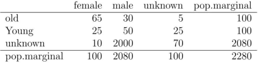
The next few tables show an hypothetical example (Micheal A. Greene, Linda E. Smith, Mark S. Levenson, Singne Hiser and Jean C. Mah) for a 2_×2 problem with an additional unknown row and unknown column. The example adjusts columns first instead of rows, but the principles are the same.

Before raking, the unknown marginal are distributed to the known marginal in proportional to the value of the known marginal and shown in Table 1. In the first

(24)

Table 1: 2_×2 problem with additional unknown row and column female male unknown pop.marginal

old 65 30 5 100

Young 25 50 25 100

unknown 10 2000 70 2080

pop.marginal 100 2080 100 2280

column of female (100 + 100_×100/2180 = 104.6) and in the second column of male (2080 + 100 _×2080/2180 = 2175.4). The table without the values of unknown is shown in Table 2. This is now ready for raking.

Table 2: Distribution of unknowns to the known marginals female male sample marginal pop.marginal

old 65 30 95 1140

Young 25 50 75 1140

sample marginal 90 80 170

pop.marginal 104.6 2175.4 2280

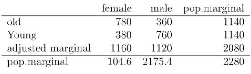
Population totals of 104.6 and 2175.4 for the columns are shown in Table 2 and are different from the computed marginals by 14.6 and 2095.4, respectively. The first iteration involves multiplying the entries in the first row by ratio of population to computed marginals as follows

ˆ N₁₁1 = n11N1· n1· = 65×1140 95 = 780, ˆ N1 12 = n12N1· n1· = 30×1140 95 = 360. Also, in the second row

ˆ N₂₁1 = n21N1· n2· = 25×1140 75 = 380, ˆ N₂₂1 = n22N1· n2· = 50×1140 75 = 760.

(25)

Then we have following results in Table 3 after first adjustment procedure. Table 3: First step in raking with rows

female male pop.marginal

old 780 360 1140

Young 380 760 1140

adjusted marginal 1160 1120 2080

pop.marginal 104.6 2175.4 2280

While the row marginal have been adjusted to the population totals, the col-umn marginal are now off. The appropriate multipliers for the colcol-umn marginal are 104.6/1160 and 2175.4/1120, respectively. This results in Table 4.

Table 4: First step in raking with columns

female male adjusted marginal pop.marginal

old 70.33 699.24 769.57 1140

Young 34.27 1476.16 1510.43 1140

pop.marginal 104.6 2175.4 2280

Table 5: Second step in raking with rows & columns

female male adjusted marginal pop.marginal

old 83.79 1048.1 1131.8 1140

Young 20.81 1127.3 1148.1 1140

pop.marginal 104.6 2175.4 2280

The application of column multipliers perfectly aligns the columns at the expense of the rows. The next iteration multiplier carries in the first row by 1140/769.57 and the second row by 1140/1510.43. In Table 5, it can be verified that one more adjustment to the columns, using multipliers 104.6/130.05 and 2175.4/2149.9 bring

(26)

the population and calculated marginals within 8.2 in both dimensions. More iterative adjustments will lead the difference to converge into very small value, ‘’, which is a given stopping rule before the procedure starts.

(27)

CHAPTER IV

STRATIFICATION AND CLUSTERING

4.1 Stratified Sampling

Many populations are, in effect, collections of populations, and a target variable in a survey may follow a different model in each of subpopulations. In a survey of households to estimate average income, for example, the income levels may vary widely among different demographic groups and regions of a country. The sample data from one subgroup may be of limit use in making estimates for other subgroups. In these populations, estimates mat be required both the full population and for some or all of the subpopulations. In either case, it is desirable to take each subpopulations as a stratum and so require a sample in each subpopulation.

The cost of conducting a survey may differ substancially among the strata. An optimum allocation of sample to the strata will consider both the cost and the variabil-ity of the target variable in each stratum. Practical problems related to response and measurement may differ considerably among subpopulations. Stratification allows some flexibility in the choice of data-collection procedures that are used for different subpopulations. Telephone data collection may be adequate for some groups while personal interviews may be needed for others, for instance. For operational conve-nience, the survey organization may also be divided into geographic district with a field office supervising work in each district.

In stratified sampling, the population is divided into nonoverlapping subpopula-tions called strata. A probability sample is selected in each stratum. The selecsubpopula-tions in different strata are independent. Stratified sampling is powerful and flexible method that is widely used in practice. In a survey, practical aspects related to response,

(28)

mea-surements, and auxiliary information may differ considerably from one subpopulation to another. Nonresponse rates and measurements problems may be more pronounced in some subpopulations than in others. The extent of the auxiliary information may differ greatly. These factors suggest that the choice of sampling design and esti-mator perhaps should be made difficulty in different subpopulations to increase the efficiency of the estimation. One may thus want to treat each subpopulation as a sep-arate stratum. For administrative reasons, the survey organization may have divided its total territory into several geographic district with a field office in each district. Here, it is natural to let each district be a stratum. An additional reason in favor of stratified sampling is that most of the potential gain in efficiency of probability proportional-to-size sampling can be captured through stratified selection with sim-ple random sampling within well-constructed strata. Stratified sampling in several respects simpler than and consequently preferred to proportional-size sampling. Let us first introduce some notation and definitions. By astratif icationof a finite popu-lationU =_{1, ..., k, ..., N_}we mean a partitioning ofU intoHsubpopulations, called strata and denoted U1, ..., Uh, ..., UH, where Uh = {k : k belongs to stratum h}. By

stratified sampling we mean that a probability samplesis selected fromUh according

to a design ph(·) (h= 1, ..., H) and that the selection in one stratum is independent

of selections in all other strata.

The resulting total sample, denoted by s as usual, will thus be composed as s=s1∪s2∪ · · · ∪sH

and, because of the independence feature,

p(s) =p1(s1)p2(s2)· · ·pH(sH).

(29)

Nh, which is assumed to be known. Since the strata form a partition ofU we have N = H X h=1 Nh.

Furthermore, the population total can be decomposed as T =X U yk = H X h=1 Th = H X h=1 Nhy¯h,

where Th is the stratum total, and ¯yh the stratum mean. Finally, let Wh = Nh/N

denote the relative size of the stratumUh. Then the population mean has the

decom-position ¯ y = H X h=1 Why¯h. 4.2 Cluster Sampling

Many naturally occuring populations exhibit clustering in which units that are near to each other (geographically or in some other respect) have similar characteristics. Households in the same neighborhood tend to have similar incomes, educational lev-els of the heads of household, and amounts of expenditures on food and clothing. Business establlishments in the same industry and geographic area will pay similar wages to a guven occupation because of competition.

In cluster population, the methods of data collection may also differ from the methods used in other populations. In household survey, for example, a complete list of households to use for sampling is usually not available, especially if the population is large. In the united states, for instance, there were nearly 100 million households in 1995. The households of interest may be geographically dispersed; field work can be more economically done when sample units are clustered together to limit travel costs. A practical and widely used technique is to select the sample in stages, using at each stage, sampling units for which a complete list is available. In the household

(30)

example, geographic areas may be selected at first stage. At the second stage, each first stage sample unit may be further subdivided and a sample of the subdivisions selected. A list of the households in each sample subdivision is then compiled and data collected from each. In a business population, establishments may be selected at the first stage, a list of occupations compiled in each sample establishment, and a sample of occupations then drawn from each list. Although occupations are the units ultimately sampled, a complete list of occupations for each establishment inthe universe is unlikely to be available, whereas a list of establishments often is. Selecting occupations in two stages can also allow better control over survey costs. Travel and extracting data from personnel records may be referred to the number of sample occupations. Two-stage sampling can also allow fine-tuning of survey budget.

A probability sample of clusters is selected, and every population element in the selected cluster is surveyed. In the single-stage cluster sampling, the finite population U =_{1, ..., k, ..., N_} is partitioned into NI clusters, and denoted U1, ..., UNI. The set

of clusters is symbolically represented as

UI ={1, ..., i, ..., NI}.

The number of population elements in the ith cluster Ui is denoted Ni. The

partitioning of U is expressed by the equations

U = [ i∈Ui Ui and N = X i∈Ui Ni.

Cluster sampling is now defined in the following way:

(1) A probability samplesI of clusters is drawn from UI according to the design

pI(·). The size of sI is denoted by nI, for a fixed size design, or by nsI for a variable

(31)

(2) Every population element in the selected clusters is observed. Here,pI(·) may

be any of conventional designs, that is, simple random sampling without replacement, systematic sampling, stratified sampling and so on.

The strategy of simple random cluster sampling is likely to be inefficient in many situations, especially if the clusters are heterogeneous or of unequal sizes. However, from a cost efficiency point of view, the strategy may have advantages, since it is often much cheaper to survey clusters of elements than to survey the geographically scattered sample that may arise from a simple random selection of elements.

However, the efficiency of cluster sampling can be improved when auxiliary infor-mation is available. The choice of strategy then depends on the inforinfor-mation available. A simple case is when an approximate measure of size ui is available for each cluster

i = 1, ..., NI. If ui is roughly proportional to ti which is the ith cluster total, we can

reduce the variance of the π- estimator (or Horvits-Thompson estimator which will be discussed later) by using probability proportional-to-size cluster sampling with inclusion probabilities πIi ∝ ui. An alternative is to use stratified cluster sampling

with strata of clusters formed so that the variation ofui is small in each stratum.

4.3 Two-stage Sampling

Cluster sampling is also called single-stage cluster sampling. By contrast, in two-stage cluster sampling, the sample of elements is obtained as result of two two-stages of sampling.

(1) The population elements are first grouped into disjoint subpopulations, called primary sampling units (PSUs). A probability sample of PSUs is drawn (first-stage sampling).

(2) For each PSU in the first-stage sampling, the type of sampling unit to be used in the second-stage sampling is decided upon. These second-stage sampling units may

(32)

be elements or clusters of elements. A probability sample of second-stage sampling units from each PSU in the first stage sample. When the second-stage sample units are clusters, every element in the selected second-stage sampling units is surveyed.

It is noted that variance of simple random sampling is smaller than simple ran-dom cluster sampling (Sarndal et al., 1992). This is explained by the tendency for elements in the same cluster to resemble each other, which implies that the homo-geneous measure is positive, and by the variation in the cluster sizes. The variance of the π estimator under simple random cluster sampling can always be reduced by selecting more clusters. However, the increased cost of taking a bigger sample may be unacceptable under the variable budget.

To control the cost and at the same time increase the number of selected clusters, we may subsample within the selected clusters, instead of surveying all elements in the selected clusters. Then we must estimate the cluster total Thi from the subsamples.

If the variation within the clusters is small, the estimates ˆThihave a smaller variance,

even for rather modest subsample sizes. It often pays to use two-stage sampling instead of cluster sampling.

Notation and estimation in two-stage sampling are slightly more complex than in cluster sampling. There are two sources of variation. The first-stage sampling vari-ation arises from the selection of primary sampling units. The second-stage sampling variation arises from the subsampling of secondary sampling units within selected PSUs.

Multistage sampling consists of three or more stages of sampling. There is a hierarchy of sampling units: primary sampling units, secondary sampling units within the PSUs, tertiary sampling units within secondary sampling units and so on. The sampling units in the last-stage sampling are called ultimate sampling units and those in the text to the last stage sampling are called penultimate sampling units.

(33)

A variety of sampling designs are available for surveys in which direct element sampling is impossible or impractical. These range from cluster sampling to highly complex multistage sampling designs using unequal probability sampling at the var-ious stages of selection. In cluster sampling, the finite population is grouped into subpopulations called clusters. Stratification and clustering both divide the popu-lation into mutually exclusive groups. Whether those groups are strata or clusters depends on how the sample is selected. If at least one sample unit is drawn from each group, they are strata. Otherwise, the groups are clusters.

(34)

CHAPTER V

POSTSTRATIFIED POINT ESTIMATOR

5.1 Population Total

Before we start to talk about point estimators, we need to define some definitions which will be used throughout later chapters. The following indexes and notations will be used in the remainder of the dissertation.

h = index for strata (h= 1, . . . , L), i= index for cluster (i= 1, . . . , Nh),

k = index for units (k = 1, . . . , Mhi),

c= index for poststrata (c= 1, . . . , C), yhikc = a variable of interest,

N =P_hNh, number of clusters in population,

M =P_hMh, population size.

We consider a clustered finite population withLstrata. LetNh be the number of

pri-mary sampling units(PSU), or clusters inh-th stratum and whik be the survey weight

associated with yhik, k-th unit within i-th cluster in h-th stratum. (An unbiased

estimator of the cluster total, Thi (i= 1, ..., nh) by subsampling in a sampled cluster

is assumed.) A stratum h contains Nh clusters. Cluster hi contains Mhi units with

Mh = PNh

i=1Mhi and M = PL

h=1Mh. In the same manner, the number of sampled

clusters inh-th stratum and sampled units inhi-th cluster arenhandmhirespectively.

(35)

sam-pling) without repllacement is also assumed. But units in different post-strata may not be iid.

However, at variance estimation stage, srs with replacement can be assumed only for computational convenience but all the assumptions maybe considered to be still valid if first-stage sampling fraction is small enough. The finite population total is T = L X h=1 Nh X i=1 Mhi X k=1 yhik = L X h=1 Th, whereTh= PNh i=1 PMhi

k=1yhik is the h-th stratum total.

An customary estimator of population total T is expressed as ˆ T = L X h=1 nh X i=1 mhi X k=1 whikyhik = L X h=1 ¯ rh = L X h=1 1 nh nh X i=1 rhi = L X h=1 ˆ Th,

where ˆTh =PN_i=1h PM_k=1hiwhikyhikis estimate of the stratum total andrhi =nhP_kwhikyhik

(one of the stratum total estimate amongnh ones based on only i-th sampled cluster

inhstratum). Note thatrhiareiidwith mean ˆTh,hstratum total, and same variance

in each stratum under with replacement sampling scheme. 5.2 Poststratified Estimator

Auxiliary variables used in the regression estimator can be both quantitative variables and qualitative variables. Actually, the poststratified estimator is a special case of

(36)

the regression estimator when the auxiliary variables are the indicator variables for the poststrata. Define the population total as

T = X

hik∈s

yhik.

We assume that the population is divided into C poststrata with size, Mc. Then the

number of units in c-th post-stratum is Mc= L X h=1 Nh X i=1 Mhi X k=1 δhikc,

where (assume design weightwhik =whifor all k) δhikc is the indicate function which

identifies if each yhik is in that poststratum or not. That is, it is defined as

δhikc =      1 if yhik ∈ c-th poststratum 0 if not .

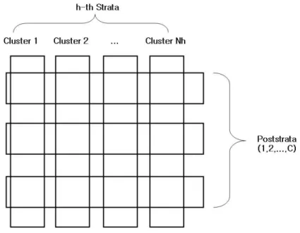
In figure 1, the structure of poststratification is graphically expressed.

(37)

Population total can be described as sum of poststrata total ˆ T = L X h=1 nh X i=1 whiTˆhi = X h X i whiMhiy¯hi = X h X i whiMhi 1 mhi X c mhi X k=1 yhikδhikc = X h X i whiMhimhic mhi X c ¯ yhic = X h X i X c Shicy¯hic = X c ˆ Tc, where ˆTc = P h P

iShicy¯hic. And if replace yhik by δhik which is indicator variable,

then we obtain estimator of Mc.

ˆ Mc = X h X i Shic =X h X i Shicδhikc ,

whereShic=whiMhimhic/mhiandmhic is the number of units in poststratumcamong

mhi units in (hi)-cluster Mc is assumed to be known and seems to be used for better

estimation. Then the poststratified estimator of the total is suggested as follows ˆ Tpst = X c ˆ RcTˆc, where ˆRc=Mc/Mˆc.

Adjustment factor ˆRcplays a very important role as balancing the weights of each

poststrata estimate cause when too many elements are selected from a poststratum, ˆ

Rc gets smaller then gives a smaller weight to poststratum estimate, ˆTc and too

small size sample from the poststratum adjusts ˆRc to be bigger for more weight. So

poststratified estimator is calculated based on the combination of both sample and population level information. GREG estimator can be expressed as following

(38)

ˆ Tw = X k∈s akyk+ (X−Xâ)0( X k∈s akxkx0k)−1 X k∈s akxkyk = Tâ+ (X−Xâ)0β,ˆ where ˆXa=P_k∈sxkak, X =P_k∈Uxk.

If we assume the auxiliary vector,xk, to be ( c−1 z }| {

0, ...,0,1,0, ...,0)0 _when _y

k is in c-th

poststratum, xk is the indicator variable and X = P

k∈Uxk is the vector of known

population total of poststrata = (M1, M2, ..., Mc)0. Let the weightak to be 1/πk, then

ˆ

Xabecomes ( ˆM1,Mˆ2, ...,Mˆc)0, where ˆMc= P

k∈sc 1

πkxkwhic is the Horvitz-Thompson

estimate of poststrata size, (M1, M2, ..., Mc)0 and ˆβ = ( ˆT1/Mˆ1,Tˆ2/Mˆ2, ...,Tˆc/Mˆc)0.

Then we are ready to show that poststratified estimator is the special case of the GREG estimator (Yung and Rao 1996). The following justifies the poststratified total estimator is the special case of the generalized regression estimator:

ˆ Tw = Tˆπ + (X−Xˆπ)0βˆ = Tˆπ +             M1 ... MC       −       ˆ M1 ... ˆ Mc             0      ˆ T1/Mˆ1 ... ˆ Tc/Mˆc       = Tˆπ + M1−Mˆ1 ˆ M1 ˆ T1+· · ·+ Mc−Mˆc ˆ Mc ˆ Tc = Tˆπ − X c ˆ Tc+ M1 ˆ M1 ˆ T1· ·+ Mc ˆ Mc ˆ Tc = X c Mc ˆ Mc ˆ Tc = Tˆpst.

(39)

CHAPTER VI

VARIANCE ESTIMATION

6.1 Variance Estimator in Estimating Population Total Then variance of ˆT is var( ˆT) = var( L X h=1 ¯ rh) = L X h=1 1 nh var(rhi) ≈ L X h=1 1 nh s2_r_hi = L X h=1 1 nh(nh−1) nh X i=1 (rhi−¯rh)2.

The variance estimator can be expressed in another way as follows: ˆ var( ˆT) = L X h=1 1 nh(nh−1) nh X i=1 (rhi−r¯h)2 = L X h=1 1 nh(nh−1) nh X i=1 ( mhi X k=1 nhwhikyhik− 1 nh nh X i=1 mhi X k=1 nhwhikyhik)2 = L X h=1 nh nh−1 nh X i=1 ( mhi X k=1 whikyhik− 1 nh nh X i=1 mhi X k=1 whikyhik)2 = L X h=1 nh nh−1 nh X i=1 (zhi−z¯h)2, wherezhi = P kwhikyhik.

6.2 The Jackknife Method

An subsample replication technique, called the jackknife, has been suggested as a broadly useful method of variance estimation. The jackknife derives estimates of the

(40)

parameter of interest from each of several subsamples of the parent sample, and then estimates the variance of the parent sample estimate from the variability between the subsamples estimates.

The jackknife is less dependent on model assumptions and does not require the formula which is usually needed by the traditional way. However, it needs repeatedly calculating the statisticntimes, which was practically impossible in the old days. The latest computing technique has made it possible for us to use the jackknife method. The jackknife has become a popular and useful tool in statistical way. Many agencies have computer software to implement the computation of the jackknife method.

The jackknife method was originally introduced to estimate the bias of an estima-tor by Quenouille(1949). It can be calculated by deleting one datum value each time fromn sampled values and reproducing the estimator using n₋1 remaining sample data. Let Tn be the estimator of unknown parameter θ based on n sample data such

as Tn = Tn(x1, x2, ..., xn−1, xn). And the bias of Tn is bias(Tn) = E(Tn)−θ. Here

we need to define one more variable Tn−1,i =Tn−1(x1, x2, .., xi−1, xi+1, .., xn) which is

based on n₋1 observations. Now we have Quenouille’s jackknife bias estimator as bj = (n−1)( ¯Tn−Tn),

where ¯Tn= _n1 Pn_i=1Tn−1,i. Also the bias reduced jackknife estimator of θ is

Tjack =Tn−bj =nTn−(n−1) ¯Tn.

The jackknife estimatorsbj and Tjack can be justified as

bias(Tjack) =bias(Tn)−E(bj) = −

b

n(n₋1)+

O

( 1 n2).

The bias of Tjack is of order _n12. The jackknife method produces a bias reduced estimator by removing the first order term in bias(Tn). Furthermore, it can lead to

(41)

the following (Shao, 1995) Tjack = nTn−(n−1) ¯Tn = nTn−(n−1) 1 n n X i=1 Tn−1,i = 1 n n X i=1 {nTn−(n−1)Tn−1,i} = 1 n n X i=1 ˜ Tn−1,i.

Tukey(1958) established that the jackknife also can be used in variance estimation and, for finite population, the jackknife technique was first introduced by Durbin (1959). Tukey suggested two conjectures to justify the jackknife variance estimation:

• T˜n,i,i= 1, ..., n are iid

• var( ˜Tn,i)≈ var(√nTn)

If these two conjectures are satisfied, the var(Tn) ≈ _n1var( ˜Tn,i). Then the jackknife

variance estimator is vjack = 1 nvar( ˜ˆ Tn,i) = 1 n(n₋1) n X i=1 ( ˜Tn,i− 1 n n X j=1 ˜ Tn,j)2 = 1 n(n₋1) n X i=1 {nTn−(n−1)Tn−1,i− 1 n n X j=1 (nTn−(n−1)Tn−1,j)}2 = 1 n(n₋1) n X i=1 {−(n₋1)Tn−1,i+ 1 n n X j=1 (n₋1)Tn−1,j}2 = n−1 n n X i=1 (Tn−1,i− 1 n n X j=1 Tn−1,j)2.

According to formula ofvar( ˆT), variance of the total estmator, ˆT, equals to sum of variances ofh strata,PL_h=1var(¯rh), which can be produced based on the assumption

(42)

that samplings between strata are independent. So jackknife method can be applied to estimate each variance of strata then jackknife variance estimate is produced by summing them up. For stratum h, jackknife variance estimator is

vjack( ˆTh) = nh−1 nh nh X i=1 ( ˆT(hi)−Tˆh)2.

Then we have the jackknife variance estimator of population total estimate vjack( ˆT) = L X h=1 nh−1 nh nh X i=1 ( ˆT(hi)−Tˆh)2,

where ˆT(hi) =Tn−1,i which is calculated based on n−1 remaining sample data after

deleting i-th cluster in h-th stratum. Furthermore, we can show that the jackknife estimator above is equivalent to the customary variance estimator by the following justification: vjack( ˆTh) = nh−1 nh nh X i=1 ( ˆT(hi)−Tˆh)2 = nh−1 nh nh X i=1 {_n 1 h−1 (zh,1+zh,2+· · ·+zh,nh−1+zh,nh −nhzh,i)} 2 = 1 nh(nh−1) nh X i=1 (nhzhi− nh X i=1 zhi)2 = 1 nh(nh−1) nh X i=1 (nh X k whikyhik− nh X i=1 X k whikyhik)2 = nh nh−1 nh X i=1 (X k whikyhik− 1 nh nh X i=1 X k whikyhik)2 = nh nh−1 nh X i=1 (zhi−z¯h)2,

wherezhi =P_kwhikyhik.

We note that in the linear case such as the population total, the customary variance estimator is equal to the jackknife estimator.

(43)

6.3 Linearization Variance Estimator

1st order Taylor series expansion for ˆRcTˆc at (Mc,Tc) is

ˆ RcTˆc=Mc ˆ Tc ˆ Mc ≈ Mc n_T_c Mc + 1 Mc ( ˆTc−Tc)− Tc M2 c ( ˆMc−Mc) o = Tc+ ˆTc− ˆ Mc Mc Tc.

Then we have the following ˆ Tpst−T = X c ( ˆRcTˆc−Tc) = X h X i 1 mhi X k X c whiMhiδhikc(yhik − ˆ Tc ˆ Mc ) = X h X i ghi =X h 1 nh X i nhghi = X h ¯ gh∗, where ghi = 1 mhi X k X c whiMhiδhikc(yhik − ˆ Tc ˆ Mc ) = X c Shic(¯yhic−µˆc) = X c Shicghic and d∗

hi(= nhdhi) are iid, i = 1, ..., nh. Then we can obtain the variance estimator of

ˆ Tpst, vL( ˆTpst) = X h 1 nh(nh−1) nh X i=1 (ghi∗ −g¯ ∗ h)2 = X h nh nh−1 nh X i=1 (ghi−¯gh)2,

provided that vL( ˆTpst −T) ≈ vL( ˆTpst). However, vL( ˆTpst) actually estimates v( ˆT),

(44)

adjusted by ˆRc=Mc/Mˆc v∗ L( ˆTpst) = X h nh nh−1 nh X i=1 n X c ˆ Rc(ghic−¯ghc) o2 , where ghic = _m1 hi P k∈shiwhiMhiδhikc(yhik− ˆ Tc ˆ Mc) =Shic(¯yhic−µˆc).

6.4 Jackknife Linearization Variance Estimator

The following is the jackknife variance estimator for the poststratified total estimator: vJ( ˆTpst) = X h nh−1 nh nh X i=1 ˆ Tpst(hi)−Tˆpst 2 = X h nh−1 nh nh X i=1 X c ˆ Rc(hi)Tˆc(hi)− X c ˆ RcTˆc 2 = X h nh−1 nh nh X i=1 n X c ( ˆRc(hi)Tˆc(hi)−RˆcTˆc) o2 , where ˆ Tpst(hi) = X c ˆ Rc(hi)Tˆc(hi) = X c Mc ˆ Mc(hi) ˆ Tc(hi).

Note that ˆMc(hi) and ˆTc(hi) are estimated after deleting (hi)-cluster and (adjusted)

linearization variance estimator is v∗ L( ˆTpst) = X h nh nh−1 nh X i=1 n X c ˆ Rc(ghic−¯ghc) o2 .

According to Valliant (1993), the standard Taylor expansion of ˆRc(hi)Tˆc(hi) at

( ˆMc, ˆTc) is ˆ Rc(hi)Tˆc(hi) = Mc ˆ Mc(hi) ˆ Tc(hi) ≈ M_ˆc Mc ˆ Tc+ Mc ˆ Mc ( ˆTc(hi)−Tˆc)− Mc ˆ Mc 2Tˆc( ˆMc(hi)−Mˆc) = RˆcTˆc+ ˆRc( ˆTc(hi)−Tˆc)−Rˆc ˆ Tc ˆ Mc ( ˆMc(hi)−Mˆc) = RˆcTˆc+ ˆRc( ˆTc(hi)−Tˆc)−Rˆcµˆc( ˆMc(hi)−Mˆc).

(45)

Also we can rewrite ˆTc as ˆ Tc = L X h=1 nh X i=1 Shicy¯hic = X h X i ˜ yhic = X h nh 1 nh X i ˜ yhic = X h nhy¯˜hc.

Then the estimate of Tc without one missing cluster is computed as

ˆ Tc(hi) = nhy¯˜hc(hi)+ X h6=h0 nh0y¯˜_h0_c = nh _n_h_y¯˜_hc₋_y_˜_hic nh−1 +X h6=h0 nh0y¯˜_h0_c = nh nh−1 (nhy¯˜hc−y¯˜hc+ ¯˜yhc−y˜hic) + X h6=h0 nh0y¯˜_h0_c = nh nh−1 (¯˜yhc−y˜hic) +nhy¯˜hc+ X h6=h0 nh0y¯˜_h0_c = nh nh−1 (¯˜yhc−y˜hic) + ˆTc. Furthermore, ˆ Tc(hi)−Tˆc = nh nh−1 (¯˜yhc−y˜hic) = ₋ nh nh−1 (˜yhic− 1 nh X i ˜ yhic) = ₋ nh nh−1 (Shicy¯hic− 1 nh X i Shicy¯hic).

By just replacing yhik by δhikc, we obtain

ˆ Mc(hi)−Mˆc=− nh nh−1 (Shic− 1 nh X i Shic).

(46)

Then plug these expressions into the standard Taylor expansion, we have ˆ

Rc(hi)Tˆc(hi) − RˆcTˆc= ˆRc( ˆTc(hi)−Tˆc)−Rˆcµˆc( ˆMc(hi)−Mˆc)

= ₋Rˆc nh nh−1 (Shicy¯hic− 1 nh X i Shicy¯hic) + ˆRcµˆc nh nh−1 (Shic− 1 nh X i Shic) = ₋Rˆc nh nh−1 Shicy¯hic− 1 nh X i Shicy¯hic −Shicµˆc+ 1 nh X i Shicµˆc = ₋Rˆc nh nh−1 n Shic(¯yhic−µˆc)− 1 nh X i Shic(¯yhic−µˆc) o .

Also, pluging this equation into the formula of the jackknife variance estimator, we finally obtain that

vJL( ˆTpst) = X h nh−1 nh X i n X c ( ˆRc(hi)Tˆc(hi)−RˆcTˆc) o2 = X h nh−1 nh X i h X c −Rˆc nh nh−1 n Shic(¯yhic−µˆc) −_n1 h X i Shic(¯yhic−µˆc) oi2 = X h nh nh−1 X i n X c ˆ Rc(ghic− 1 nh X i∈sh ghic) o2 = L X h=1 nh nh−1 nh X i=1 n X c ˆ Rc(ghic−g¯hc) o2 = v∗ L( ˆTpst).

(47)

6.5 New Proposed Linearization Variance Estimator

Furthermore, we considered 2nd order Taylor series expansion for ˆRcTˆc at (Mc, Tc)

which is evaluated as ˆ RcTˆc=Mc ˆ Tc ˆ Mc ≈ Mc n_T_c Mc + 1 Mc ( ˆTc−Tc)− Tc Mc2 ( ˆMc−Mc) + Tc Mc3 ( ˆMc−Mc)2− 1 Mc2 ( ˆTc−Tc)( ˆMc−Mc) o = Tc+ ˆTc− ˆ Mc Mc Tc + Tc Mc2 ( ˆMc−Mc)2− 1 Mc ( ˆTc−Tc)( ˆMc−Mc) = Tc+ ˆTc(2− ˆ Mc Mc ) +Tc n_Mˆ_c Mc 2 −2Mˆc Mc o = Tc+ (2− ˆ Mc Mc )( ˆTc− ˆ Mc Mc Tc). Then, we have ˆ Tpst−T = X c ( ˆRcTˆc−Tc) = X c (2₋ Mˆc Mc )( ˆTc− ˆ Mc Mc Tc) = X h X i X c X k whiMhi mhi (yhikδhikc− ˆ Tc ˆ Mc )(2₋ 1 ˆ Rc ) = X h X i 1 mhi X c (2₋ 1 ˆ Rc )Shic(¯yhic−µˆc) = X h X i ghi= X h 1 nh X i nhghi = X h ¯ g_h∗, where ghi= _m1 hi P c(2− 1 ˆ

Rc)Shic(¯yhic−µˆc) and ˜g ∗

(48)

Therefore, variance of ˆTpst is vL∗∗( ˆTpst) = X h 1 nh(nh−1) nh X i=1 (ghi∗ −¯g ∗ h)2 = X h nh nh −1 nh X i=1 (˜ghi−¯gh)2 = X h nh nh −1 nh X i=1 n X c (2₋ 1 ˆ Rc )(ghic−g¯hc) o2 .

Comparing this to the standard linearization estimator, the second-order lin-earization variance estimator has the function of the adjustment factor, 2₋1/Rc.

This function works like the ratio, Rc, but slightly different. If the value of Rc is

around 1, both have the values close to 1. But for extremely unbalanced case such that the values are far from 1, 2₋1/Rc gives smaller weights for each poststratum.

So 2₋1/Rc also has the functionality of balancing weights for poststrata which can

reduce the bias from the unbalanced sampling. Rao’s adjusted variance estimator can be obtained by adding the ratio adjustment factor, Rc to the standard linearization

variance estimator. We note thatMc/Mˆcconverges in probability to 1. So, there is no

harm in switchingvL to vL∗ since v ∗

L is asymptotically equivalent to vL. If the Taylor

expansion is expanded to the second-order, we have the new linearization variance estimator with the function, 2₋1/Rc. This function came from the process of the

second-order Taylor approximation. So the second-order estimator has the function which balances weights for the poststrata while the standard linearization variance estimator,vL, does not have. We know that the new variance estimator is equivalent

to v∗

L and vL. Because the function, 2−1/Rc, also converges in probability to 1.

Therefore, its adjusted version also can be suggested as vadj,L∗∗ ( ˆTpst) = X h nh nh−1 nh X i=1 n X c ˆ Rc(2− 1 ˆ Rc )(ghic−¯ghc) o2 , where ghic = _m1 hi P k∈shiwhiMhiδhikc(yhik − Tc Mc) = Shic(¯yhic −µˆc). vL( ˆTpst), v ∗∗ L( ˆTpst)

(49)

and v∗∗

adj,L( ˆTpst) are all asymptotically equivalent, because ˆRc p

→1.

We also can consider that poststratification is made across on the clusters, not the units within cluster.

Mc = X h Nh X i=1 Mhi X k=1 δhic = X h Nh X i=1 δhicmhi.

Then, population total estimator, ˆT can be expressed in different way as follows, ˆ T = X h nh X i=1 whiTˆhi = X h X i whiMhiy¯hi = X c X h X i Shiδhicy¯hi = X c ˆ Tc. Now we know ˆ Tc = X h X i Shiδhicy¯hi.

By replacing ¯yhi by δhic, then

ˆ Mc = X h X i Shi =X h X i Shiδhic ,

which is identical to ˆMc when mhic =mhi (Shi=whiMhi ). Therefore,

vL( ˆTpst) = X h 1 nh(nh−1) nh X i=1 (ghi∗ −g¯ ∗ h··)2 = X h nh nh−1 nh X i=1 (ghi−g¯h·)2.

We also apply second order linearization to jackknife variance estimator. By linearizing, second-order jackknife linearization variance estimator can be obtained.

(50)

Second-order Taylor expansion of ˆRc(hi)Tˆc(hi) at ( ˆMc, ˆTc) is ˆ Rc(hi)Tˆc(hi) = Mc ˆ Mc(hi) ˆ Tc(hi) ≈ M_ˆc Mc ˆ Tc+ Mc ˆ Mc ( ˆTc(hi)−Tˆc)− Mc ˆ Mc 2Tˆc( ˆMc(hi)−Mˆc) + Tˆc ˆ M3 c ( ˆMc(hi)−Mˆc)2− 1 ˆ M2 c ( ˆTc(hi)−Tˆc)( ˆMc(hi)+ ˆMc) = RˆcTˆc+ ˆRc n ˆ Tc(hi)−Tˆc− ˆ Tc ˆ Mc ˆ Mc(hi)+ ˆTc + Tˆc ˆ M2 c ( ˆMc(hi)−Mˆc)2− 1 ˆ Mc ( ˆTc(hi)−Tˆc)( ˆMc(hi)+ ˆMc) o = RˆcTˆc+ ˆRc n ˆ Tc(hi)− ˆ Mc(hi) ˆ Mc ˆ Tc+ ˆ M2 c(hi) ˆ M2 c ˆ Tc+ ˆTc−2 ˆ Mc(hi) ˆ Mc ˆ Tc −Mˆc(hi)_ˆ Mc ˆ Tc(hi)+ ˆTc(hi)+ ˆ Mc(hi) ˆ Mc ˆ Tc−Tˆc o = RˆcTˆc+ ˆRc n 2Tˆc(hi)− ˆ Mc(hi) ˆ Mc ˆ Tc − Mˆc(hi)_ˆ Mc ˆ Tc(hi)− ˆ Mc(hi) ˆ M ˆ Tc o = RˆcTˆc+ ˆRc n 2₋ Mˆc(hi) ˆ Mc ˆ Tc(hi)− ˆ Mc(hi) ˆ Mc ˆ Tc o . Then we have ˆ Rc(hi)Tˆc(hi)−RˆcTˆc = ˆRc 2₋ Mˆc(hi) ˆ Mc ˆ Tc(hi)− ˆ Mc(hi) ˆ Mc ˆ Tc . Therefore, v∗ JL( ˆTpst) = X h nh−1 nh nh X i=1 n X c ( ˆRc(hi)Tˆc(hi)−RˆcTˆc) o2 ≈ X h nh−1 nh nh X i=1 n X c ˆ Rc 2₋ Mˆc(hi) ˆ Mc ˆ Tc(hi)− ˆ Mc(hi) ˆ Mc ˆ Tc o2 .

The second-order jackknife linearization variance estimator is very similar to the adjusted version of the second order linearization variance estimator that we proposed

(51)

before. It has ˆMc(li)/Mˆcand ˆTc(li)instead of ˆMc/Mcand ˆTc(li). However,vJL∗ needs to

compute ˆMc(li)and ˆTc(li)which require extensive calculations as the standard jackknife

estimator does. So it may not be preferred to the jackknife variance estimator with respect to time and cost.

(52)

CHAPTER VII

SIMULATION STUDY I

To observe and compare the performances of variance estimators which include the standard linearization estimtor vL, the jackknife linearization estimatorvJL, the

sec-ond order linearization estimator v∗∗

L and its adjusted version v∗∗adj,L , we generate

a population with 50,000 with four poststrata. The values of yhik are generated

from four different normal distributions (poststrata) with given means (µ1, µ2, µ3,

µ4)=(40, 60, 80, 100) and standard deviations (σ1, σ2, σ3, σ4)=(8.94, 10.95, 12.65,

14.14). Poststrata sizes are randomly determined and assigned as (9,561, 18,800, 6,163, 15,476) respectively. All 50,000 units are randomly apportioned into 10 strata and 800 clusters with equal probabilities. Consequently, each stratum has 80 clusters and cluster size varies from 40 to 89. After the clustered population is obtained, iterative drawings of sample should be carried under designed sampling plan.

First, we consider one-stage sampling scheme. One-stage is a special case of two-stage sampling design. Because if all the units are selected within sampling clusters under two-stage sampling design, this becomes a single stage. The largest cluster size of the generated population is 89. If we select 89 units within all the sampling clusters, which covers all the units in, that is equivalent to one-stage cluster sampling. Hence, calculations of variance estimators for both one-stage and two-stage are carried in the same manner. In one-stage sampling, we selected 1,000 independent samples. At each sample, nh clusters were selected from each hth-stratum with probability

proportional to cluster size. We repeated this with four different numbers of sampling clusters nh = 4,6,8,10 respectively, fori= 1, ...,10 per stratum with selecting all the

(53)

The sampling method used under two-stage cluster sampling plan is thatppsat first stage and srs at second stage. This yields equal selection probabilities for all units. The selection probability of j-th unit ini-th cluster is

πij = nMi M mhi Mi = nmhi M .

Eight clusters per stratum are selected with pps so total eighty clusters out of eight hundreds population clusters are sampled at the first stage. For each sampling cluster, mhi = 6,10,14,18 units within cluster are drawned respectively. If number of units

in a cluster is smallermhi, all the units in that cluster are taken. So total sample size

for each time of sampling is not fixed but similar. Empirical mean sqaure error or say ‘vE’ is calculated for each variance estimator based on 1,000 samples defined by

vE = 1 1000 1000 X i=1 ( ˆTpst,i−T)2,

where ˆTpst,i is the estimated total for the i-th generated sample (i = 1,2, ...,1000).

Mean sqaure error and relative bias are used to measure the precision and performance for each variance estimator based on the sample size.

MSE = 1 1000 1000 X i=1 (ˆvi−vE)2, Relative bias = 1 1000 P ivi vE − 1,

(54)

The second order linearization estimator, v∗∗

L, performs as well as vL and vJL

for both one and two-stage. We also used a real finite population which is called third grade population. It consists of 2,427 students who participated in the Third International Mathematics and Science Study (Caslyn, Gonzales and Frase, 1999). The methods used in conducting the original study are given in TIMSS International Study Center (1996). The population consists of only students from the United States and it has four regions which are strata. Clusters are schools while units within clus-ters are the students. We limit the variable of interest be the total math score of the population and let the poststrata to be the ethics which has eight categories in this study. n1 = 11, n2 = 16, n3 = 10, n4 = 23 clusters are selected from stratum with

proportional allocation andm= 4,8,12,16 units are sampled within each cluster, re-spectively. 1,000 simulations for each different number of sampling units shows similar result to simulated population. v∗∗

L still estimates the variance of the poststratified

estimator well.

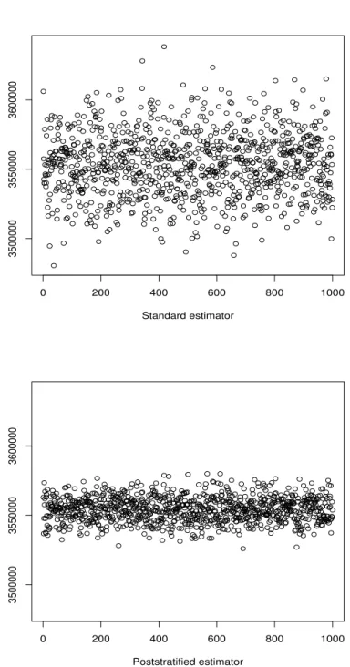
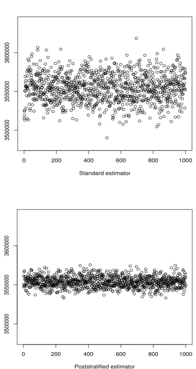
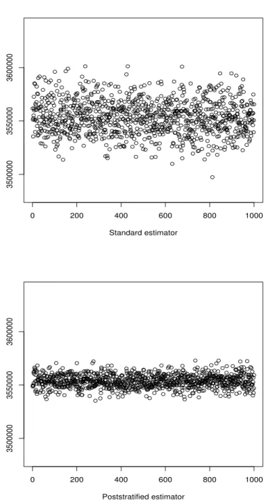
In Tables 6 and 7 and from Figures 2 to 9, poststratified estimator shows much better performance than standard estimator. Performances of the variance estimators are shown in Tables 8 and 9 and from Figures 10 to 14. We also recorded the results of the simulations on the third grade data in Tables 10 and 11.

(55)

Table 6: Point estimators at one-stage on the simulated population ˆ T Tˆpst Relative bias m = 4 -0.01 0.00 m= 6 0.00 0.00 m= 8 -0.01 0.00 m= 10 -0.01 0.00 M SE(_÷107₎ _n_{= 4} _51.7 _8.09 n= 6 33.3 5.19 n= 8 25.8 3.87 n= 10 18.2 2.80

Table 7: Point estimators at two-stage on the simulated population

ˆ T Tˆpst Relative bias m= 6 -0.01 0.00 m = 10 -0.01 -0.01 m = 14 -0.01 0.00 m = 18 0.00 0.00 M SE(_÷108₎ _m _{= 6} _30.34 _4.00 m = 10 17.96 2.71 m = 14 12.55 1.73 m = 18 8.74 1.39

(56)

Table 8: Variance estimators at one-stage on the simulated population VL VJL VL∗∗ Vadj,L∗∗ Relative bias m= 4 0.002 0.002 0.001 0.003 m= 6 0.021 0.021 0.020 0.022 m= 8 0.022 0.022 0.021 0.022 m= 10 0.076 0.076 0.075 0.076 M SE(_÷1013₎ _m_{= 4} _{16.17 16.09 16.04 16.18} m= 6 4.300 4.284 4.238 4.335 m= 8 1.890 1.894 1.876 1.922 m= 10 2.841 2.838 2.814 2.860

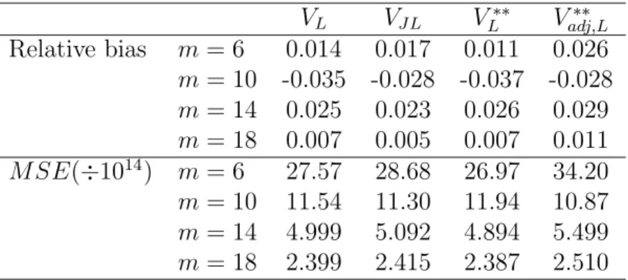
Table 9: Variance estimators at two-stage on the simulated population

VL VJL VL∗∗ V ∗∗ adj,L Relative bias m = 6 0.014 0.017 0.011 0.026 m = 10 -0.035 -0.028 -0.037 -0.028 m = 14 0.025 0.023 0.026 0.029 m = 18 0.007 0.005 0.007 0.011 M SE(_÷1014₎ _m _{= 6} _27.57 _28.68 _26.97 _34.20 m = 10 11.54 11.30 11.94 10.87 m = 14 4.999 5.092 4.894 5.499 m = 18 2.399 2.415 2.387 2.510

(57)

Table 10: Point estimators at two-stage on the third grade population ˆ T Tˆpst Relative bias m= 4 -0.01 -0.01 m= 12 -0.01 -0.01 M SE(_÷108₎ _n_{= 4} _2.45 _2.00 n= 12 1.75 1.26

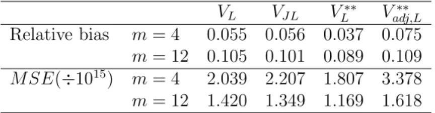
Table 11: Variance estimators at two-stage on the third grade population, n1 =

11, n2 = 16, n3 = 10, n4 = 23 VL VJL VL∗∗ Vadj,L∗∗ Relative bias m= 4 0.055 0.056 0.037 0.075 m= 12 0.105 0.101 0.089 0.109 M SE(_÷1015₎ _m_{= 4} _{2.039 2.207 1.807 3.378} m= 12 1.420 1.349 1.169 1.618

(58)

0 200 400 600 800 1000 3500000 3550000 3600000 Standard estimator 0 200 400 600 800 1000 3500000 3550000 3600000 Poststratified estimator

Figure 2: Point estimates of population total on 1,000 samples from the simulated population under one-stage cluster sampling,n = 4

(59)

(60)

(61)

0 200 400 600 800 1000 3500000 3550000 3600000 Poststratified estimator 0 200 400 600 800 1000 3500000 3550000 3600000 Poststratified estimator

(62)

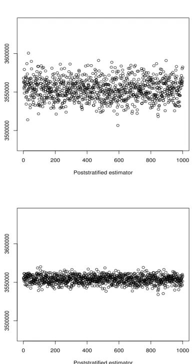
0 200 400 600 800 1000 3400000 3500000 3600000 3700000 Standard estimator m=6 0 200 400 600 800 1000 3400000 3500000 3600000 3700000 Poststratified estimator m=6

Figure 6: Point estimates of population total on 1,000 samples from the simulated population under two-stage cluster sampling, selecting eight clusters per stratum and m= 6 units in each cluster

(63)

0 200 400 600 800 1000 3400000 3500000 3600000 3700000 Standard estimator m=10 0 200 400 600 800 1000 3400000 3500000 3600000 3700000 Poststratified estimator m=10

Figure 7: Point estimates of population total on 1,000 samples from the simulated population under two-stage cluster sampling, selecting eight clusters per stratum and m= 10 units in each cluster