2014
Doubly robust inference with missing data in
survey sampling
Jae Kwang Kim
Iowa State University, [email protected]
David Haziza
Universite de Montreal
Follow this and additional works at:
http://lib.dr.iastate.edu/stat_las_pubs
Part of the
Design of Experiments and Sample Surveys Commons
, and the
Multivariate Analysis
Commons
The complete bibliographic information for this item can be found at
http://lib.dr.iastate.edu/
stat_las_pubs/111
. For information on how to cite this item, please visit
http://lib.dr.iastate.edu/
howtocite.html
.
This Article is brought to you for free and open access by the Statistics at Iowa State University Digital Repository. It has been accepted for inclusion in Statistics Publications by an authorized administrator of Iowa State University Digital Repository. For more information, please contact
doi:http://dx.doi.org/10.5705/ss.2012.005
DOUBLY ROBUST INFERENCE WITH MISSING DATA IN SURVEY SAMPLING
Jae Kwang Kim and David Haziza
Iowa State University and Universit´e de Montr´eal
Abstract: Statistical inference with missing data requires assumptions about the population or about the response probability. Doubly robust (DR) estimators use both relationships to estimate the parameters of interest, so that they are consistent even when one of the models is misspecified. In this paper, we propose a method of computing propensity scores that leads to DR estimation. In addition, we discuss DR variance estimation so that the resulting inference is doubly robust. Some asymptotic properties are discussed. Results from two limited simulation studies are also presented.
Key words and phrases: Calibration, double protection, nonresponse, variance es-timation.
1. Introduction
Missing data occurs in surveys because some of the sampled units refuse to respond to the survey or because of the inability to contact them. Dropout or noncompliance in clinical trials may also lead to missing responses for some subjects. It is well known that unadjusted estimators may be heavily biased if the respondents differ from the nonrespondents systematically with respect to the study variables. It is thus desirable to develop estimation procedures exhibiting low biases.
To adjust for the bias associated with missing data, two modeling approaches are often used: the response probability (RP) model approach that requires the specification of a response model describing the unknown nonresponse mechanism and the outcome regression (OR) model approach that requires the specification of the model describing the distribution of the study variable. In survey sam-pling the RP model approach is also called the nonresponse model approach, whereas the OR model approach is called the prediction model approach or the imputation model approach. An estimator is said to be doubly robust (DR) if it remains asymptotically unbiased and consistent if either model (nonresponse or outcome regression) is true. DR procedures offer some protection against mis-specification of one model or the other. This is clearly an attractive property and is closely related with the philosophy of model-assisted estimation in survey
sampling (S¨arndal, Swensson and Wretman (1992); Firth and Bennett (1998); Fuller (2009)).
In recent years, DR estimation procedures have attracted a lot of attention in mainstream statistics; e.g., Robins, Rotnitzky, and Zhao (1994), Scharfstein, Rotnitzky, and Robins (1999), Tan (2006), Bang and Robins (2005), Kang and Schafer (2008), Cao, Tsiatis, and Davidian (2009), among others. In the survey sampling context, DR estimation has been studied in Kott (1994), Kott (2006), Kott and Chang (2010), Kim and Park (2006), and Haziza and Rao (2006), among others. Kott (2006) discussed the doubly robustness of the variance estimator proposed by Folsom and Singh (2000) in the context of calibration for unit non-response in survey sampling; see also Kott and Chang (2010). In the context of imputation for missing data, DR variance estimation has been discussed in Haz-iza and Rao (2006) and Kim and Park (2006) when the overall sampling fraction is negligible. Haziza and Rao (2006) considered Taylor linearization procedures, whereas replication variance estimation was studied in Kim and Park (2006). However, Haziza and Rao (2006) and Kim and Park (2006) did not address the double robustness of the variance estimators for large sampling fractions.
We consider DR inference in the sense that the inference based on point estimator and variance estimator is justified if either one of the two models, non-response model or outcome regression model, holds. The proposed doubly robust estimator is quite efficient and provides a variance estimator that can be easily implemented using software designed for complete data variance estimation. In finite population sampling, the proposed variance estimator is slightly modified. In Section 2, the basic setup is introduced. The proposed DR estimator and its variance estimator are discussed in Section 3. In Section 4, the proposed method is applied to the survey sampling context and the proposed variance estimator is modified to account for the finite population. Results from two simulation studies are presented in Section 5 to compare the performance of the proposed estimator with those from existing methods. Concluding remarks are made in Section 6.
2. Basic Setup
Suppose we have nindependent realizations of a random variableY,y1, . . .,
yn, from some distribution, and that we are interested in estimatingθ=E(Y). In
the absence of nonresponse to the study variabley, the parameterθis consistently estimated by the sample mean
ˆ θn= n ∑ i=1 wiyi, (2.1)
where wi = 1/n. In Section 4, we use a different set of weights wi as we treat
In addition to the study variable y, suppose a vector of auxiliary variables, x, is available in the sample. Let δi be a response indicator attached to unit i
such that δi = 1 if yi is observed and δi = 0, otherwise. Instead of observing
(xi, yi) for the whole sample, we observe (xi, yi) forδi= 1 and observe onlyxifor
δi = 0. We assume that the response mechanism is missing at random (MAR)
in the sense of Rubin (1976).
A natural approach for estimating θconsists of first postulating a model for the conditional distribution ofyigivenxi. In particular, if we are only interested
in the mean of the y-values, we consider the following model
E(yi |xi, δi= 0) =m(xi;β0), (2.2)
where m(xi,β) is a continuous differentiable function of β. The model (2.2) is
called the OR model. Under MAR, (2.2) implies that E(yi|xi) =m(xi;β0).
A natural estimator of θ is the (deterministically) imputed estimator ˆ θp= n ∑ i=1 wi { δiyi+ (1−δi)m(xi,βˆ) } , (2.3)
where ˆβ is a consistent estimator of the true parameter β0. Since ˆ θp−θˆn=− n ∑ i=1 wi(1−δi) { yi−m(xi,βˆ), } we have E { ˆ θp−θˆn|δ1, . . . , δn,x1, . . . ,xn } =− n ∑ i=1 wi(1−δi) { E(yi|xi, δi= 0)−m(xi,βˆ) } ,
where E(· | δ1, . . . , δn,x1, . . . ,xn) denotes the conditional expectation with
re-spect to the OR model. Thus, the validity of the imputed estimator (2.3) follows if (2.2) is true and ˆβ is a consistent estimator ofβ0.
Now, suppose that the probability of response to the study variable y,pi =
Pr (δi= 1|xi), follows a parametric model
pi =pi(ϕ0) =
exp(ϕ′0xi
)
1 + exp(ϕ′0xi
) (2.4)
for some ϕ0. The model (2.4) is called the RP model. We assume that the intercept term is included in (2.4). In the classical two-phase sampling setup, where the phase sample corresponds to the set of respondents, the second-phase conditional inclusion probabilitypi is known and the two-phase regression
ˆ θtp= n ∑ i=1 wi [ m(xi; ˆβ) + δi pi { yi−m(xi; ˆβ) }] = ˆθn+ n ∑ i=1 wi (δ i pi − 1){yi−m ( xi; ˆβ )} (2.5) is approximately unbiased for θ under the nonresponse model (Cochran (1977)) regardless of whether or not (2.2) holds. When the RP model is not correct, the estimator is still approximately unbiased if (2.2) and the MAR condition hold and ˆβis consistent forβ0. Thus, ˆθtpis doubly robust in the sense that it remains
valid if either one of the two models holds.
When the response probability is estimated, rather than known, we consider a class of estimators of the form
ˆ θDR( ˆβ,ϕˆ) = ˆθn+ n ∑ i=1 wi { δ i pi( ˆϕ) −1 } { yi−m ( xi; ˆβ )} , (2.6)
indexed by ( ˆβ,ϕˆ), where ˆβis consistent forβ0under the assumed OR model and ˆ
ϕ is consistent for ϕ0 under the assumed RP model. As noted by Scharfstein, Rotnitzky, and Robins (1999), the double robustness property also follows if pi
is replaced by ˆpi = pi( ˆϕ) using a consistent estimator ˆϕ for ϕ0. Note that
the doubly robust estimator, ˆθDR( ˆβ,ϕˆ), in (2.6) is a class of estimators and
different choices of ( ˆβ,ϕˆ) lead to different doubly robust estimators. Scharfstein, Rotnitzky, and Robins (1999) and Haziza and Rao (2006) used ˆϕ estimated by maximum likelihood and ˆβestimated by ordinary or iteratively reweighted least squares. Recently, Cao, Tsiatis, and Davidian (2009) proposed a doubly robust estimator using the optimal score equation based on influence function theory. However, the proposed variance estimator of Cao, Tsiatis, and Davidian (2009) is not necessarily doubly robust.
We propose a DR estimator of the form (2.6) using a different choice of ( ˆβ,ϕˆ) which leads to a simplified DR variance estimator. Thus, the proposed point and variance estimation procedure leads to DR inference.
3. Main Results Let S(ϕ)≡ n ∑ i=1 wi { δi pi(ϕ)− 1 } hi(ϕ) = 0 (3.1)
be the (weighted) score equation forϕ0, wherehi(ϕ) ={∂pi(ϕ)/∂ϕ}/{1−pi(ϕ)}.
Given the choice of ˆpi =pi( ˆϕM LE) where ˆϕM LE satisfies (3.1), Cao, Tsiatis, and
Davidian (2009) considered so-called the optimal DR estimator among the class of the estimators of the form
ˆ θDR( ˆβ) = n ∑ i=1 wi { m ( xi; ˆβ ) +δi ˆ pi (yi−m(xi; ˆβ)) } . (3.2) Rubin and van der Laan (2008) considered the ˆβ that minimizes
n ∑ i=1 wi2δi ˆ pi (1 ˆ pi − 1 ) {yi−m(xi;β)}2,
which is essentially the conditional variance ignoring the effect of estimatingϕ0
in the estimated response probability ˆpi = pi( ˆϕ). To correctly account for the
effect of estimating ϕ0, Cao, Tsiatis, and Davidian (2009) proposed minimizing
n ∑ i=1 w2i δi ˆ pi (1 ˆ pi − 1 ) { yi−m(xi;β)−c′hi( ˆϕM LE) }2
with respect to (β,c). Note that in this case there is no guarantee that the resulting estimator is optimal under the OR model. In fact, the proposed es-timator of Cao, Tsiatis, and Davidian (2009) is sub-optimal because they first estimate ˆϕ by ˆϕM LE obtained from maximum likelihood and then seek for the optimal estimator in the class of estimators ˆθ∗DR( ˆβ) = ˆθDR( ˆβ,ϕˆM LE) as a
func-tion of ˆβ. As discussed in Kim and Kim (2007) and Kim and Riddles (2012), the choice of ˆϕM LE does not necessarily lead to the optimal propensity score estimators. For example, according to Kim and Riddles (2012), when the OR model ism(xi;β) =x′iβ, the optimal choice of ˆϕcan be obtained by solving
n ∑ i=1 wi δi pi(ϕ) xi = n ∑ i=1 wixi, (3.3)
which is different from the score equation for the MLE of ϕ0. Thus, we expect that the efficiency of the sub-optimal estimator of Cao, Tsiatis, and Davidian (2009) can be improved for a suitable choice of ˆϕ.
We propose a DR estimator ˆθp of the form (2.3) using ( ˆβ,ϕˆ), where ( ˆβ,ϕˆ)
is obtained by solving n ∑ i=1 wiδi { 1 pi(ϕ)− 1 } {yi−m(xi;β)}xi=0, (3.4) n ∑ i=1 wi { δ i pi(ϕ) − 1 } ˙ m(xi;β) =0, (3.5)
simultaneously, where ˙m(xi;β) = ∂m(xi;β)/∂β. Because an intercept term is
included inx, (3.4) implies that
n ∑ i=1 wiδi 1 pi( ˆϕ) { yi−m(xi; ˆβ) } = n ∑ i=1 wiδi { yi−m(xi; ˆβ) } .
Thus, by (3.4), the imputed estimator (2.3) can be expressed as a doubly robust estimator of the form (2.6).
Condition (3.4) has been used in Scharfstein, Rotnitzky, and Robins (1999) and Haziza and Rao (2006). Condition (3.5) is a calibration condition in the sense that the propensity score adjusted estimator applied to ˙m(xi;β) leads
to the complete sample estimator. For example, consider the linear OR model for which m(xi;β) = x′iβ. Then, (3.5) is equivalent to (3.3). Condition (3.3)
was considered by Folsom (1991), Iannacchione, Milne, and Folsom (1991), and Chang and Kott (2008) in the context of unit nonresponse in survey sampling. From (3.3), it follows that estimates corresponding to the x-variables do not suffer from nonresponse error. Condition (3.4) means that ˆβ is computed as
ˆ β= {∑n i=1 δi(ˆp−i 1−1)xix′i }−1∑n i=1 δi(ˆp−i 1−1)xiyi.
Writingyi =x′iβ0+ei, the imputed estimator ˆθp can be written as
ˆ θp= ˆθn+ n ∑ i=1 wi { δ i pi( ˆϕ) −1 } x′i ( β0−βˆ ) + n ∑ i=1 wi { δ i pi( ˆϕ) −1 } ei.
Note that the second term here is zero if (3.5) holds. Thus, under (3.5), ˆ θp= ˆθn+ n ∑ i=1 wi { δi pi( ˆϕ) −1 } ei
and the variability associated with ˆβ can be safely ignored. Furthermore, using the fact ∂p−i1(ϕ)/∂ϕ =−{p−i 1(ϕ)−1}xi under (2.4), we can apply a Taylor
expansion to get ˆ θp= ˆθn+ n ∑ i=1 wi { δi pi(ϕ∗)− 1 } ei− n ∑ i=1 wiδi { 1 pi(ϕ∗)− 1 } eixi ( ˆ ϕ−ϕ∗ ) +Op ( n−1), (3.6) whereϕ∗ is the probability limit of ˆϕ. Using (3.4), it can be shown that
n ∑ i=1 wiδi { 1 pi(ϕ∗)− 1 } eixi =op(1) and (3.6) reduces to ˆ θp = ˆθn+ n ∑ i=1 wi { δ i pi(ϕ∗) − 1 } ei+op ( n−1/2 ) . (3.7)
Thus, the variability associated with ˆϕcan also be safely ignored.
We need some regularity conditions. The following theorem extends the above results to the general form ofE(yi|xi) =m(xi;β0).
Assume the following regularity conditions:
(C.1) There is a fixed constant KB such that p−i 1< KB for all i= 1,2, . . . , n.
(C.2) The response probability function pi(ϕ) is differentiable with continuous
first order partial derivatives for all ϕ.
(C.3) The solution ( ˆβ,ϕˆ) to (3.4) and (3.5) is uniquely determined and satisfies ( ˆβ,ϕˆ) = (β∗,ϕ∗) +op(1) for some (β∗,ϕ∗).
(C.4) The mean functionm(xi;β) is twice differentiable with continuous
second-order partial derivatives for all β.
(C.5) W(β) = (X, Y, m(x;β),m˙(x;β)) has finite fourth moment for all β. Theorem 1. Under (C.1)−(C.5), we have
√ n ( ˆ θp−θ˜p ) =op(1), (3.8) where ˜ θp= n ∑ i=1 wi [ m(xi;β∗) + δi pi(ϕ∗){ yi−m(xi;β∗)} ] (3.9)
and (β∗,ϕ∗) is the probability limit of( ˆβ,ϕˆ).
Proof. Write the DR estimator as ˆθp = ˆθp( ˆβ,ϕˆ), where ( ˆβ,ϕˆ) is the solution to
(3.4) and (3.5). Now, if U(β,ϕ) = n ∑ i=1 wi ( δ i pi(ϕ) − 1 ) {yi−m(xi;β)}, we can write ˆ θp( ˆβ,ϕˆ) = ˆθn+U( ˆβ,ϕˆ). (3.10)
Note thatU(β,ϕ) satisfies ∂ ∂ϕU(β,ϕ) =− n ∑ i=1 wiδi {1−pi(ϕ) pi(ϕ) } {yi−m(xi;β)}xi, ∂ ∂βU(β,ϕ) =− n ∑ i=1 wi { δ i pi(ϕ) − 1 } ˙ m(xi;β).
Thus, conditions (3.4) and (3.5), are equivalent to ∂
Because of the existence of the second moment of the partial derivatives in (3.11), standard arguments for the asymptotic normality of ( ˆβ,ϕˆ) can be used to show that ( ˆβ,ϕˆ)−(β∗,ϕ∗) =Op ( n−1/2 ) . (3.12) Because ( ˆβ,ϕˆ) satisfies (3.11), its probability limit (β∗,ϕ∗) satisfies
E
{ ∂
∂(β,ϕ)U(β,ϕ)|β=β
∗,ϕ=ϕ∗}=0. (3.13)
Condition (3.13) that implies that the contribution due to estimating the param-eters (β,ϕ) is negligible in the asymptotic distribution ofU(β,ϕ), is often called Randles (1982) condition. From (3.12) and (3.13), we obtain
U( ˆβ,ϕˆ) =U(β∗,ϕ∗) +op(n−1/2). (3.14)
Therefore, combining (3.10) and (3.14), we have (3.8).
The probability statement in (3.8) is made in the doubly robust sense that the convergence in probability holds if one of the two models is true. If the reference distribution in (3.8) is with respect to (2.2), then β∗ = β0. If the reference distribution in (3.8) is with respect to (2.4), then ϕ∗ =ϕ0. When the two models are true, then (β∗,ϕ∗) = (β0,ϕ0) and the variance of ˜θp is
V ( ˜ θp ) =V ( ˆ θn ) +E {∑n i=1 wi2{pi(ϕ0)−1−1}e2i } , (3.15)
where ei = yi−m(xi;β0). Under simple random sampling, (3.15) is equal to
the semiparametric lower bound of the asymptotic variance and, as a result, ˆθp
is locally efficient (Robins, Rotnitzky, and Zhao (1994)). Taking ηi(β,ϕ) =m(xi;β) + δi pi(ϕ){ yi−m(xi;β)}, (3.16) (3.8) means that n ∑ i=1 wiηi( ˆβ,ϕˆ) = n ∑ i=1 wiηi(β∗,ϕ∗) +op ( n−1/2 ) .
Thus, if (xi, yi, δi) are i.i.d., theηi(β∗,ϕ∗) are i.i.d., even thoughηi( ˆβ,ϕˆ) are not
necessarily i.i.d.. Because ηi(β∗,ϕ∗) are i.i.d., we can apply the Central Limit
Theorem and the Slutsky Theorem to get √ n ( ˆ θp−θ ) L →N(0, σ2), (3.17)
where →L denotes the convergence in distribution and σ2 = V ar{ηi(β∗,ϕ∗)}.
Furthermore, since ηi(β∗,ϕ∗) are i.i.d with bounded fourth moments, we can
apply the standard complete sample method to estimate the variance of ˜θp =
∑n i=1wiηi(β∗,ϕ∗). Then ˆ V(β∗,ϕ∗) = 1 n 1 n−1 n ∑ i=1 (ηi−η¯n)2, (3.18) whereηi =ηi(β∗,ϕ∗) and ¯ηn=n−1 ∑n i=1ηi, satisfies ˆ V(β∗,ϕ∗) V p →1,
whereV =n−1σ2 and →p denotes the convergence in probability. Therefore, by the Slutsky Theorem again, we have
ˆ θp−θ √ ˆ V( ˆβ,ϕˆ) L →N(0,1). (3.19) This asymptotic result can be used to construct confidence intervals forθ=E(Y). The reference distribution in (3.19) is either the OR model or the RP model.
The variance estimator (3.18) of the proposed DR estimator is computation-ally attractive because the linearized values, (3.16), are easy to compute. 4. Extension to Survey Sampling
We consider the problem of doubly robust inference in the survey sampling context. Consider a finite populationU of sizeN. We are interested in estimating the mean of the finite population, θN =N−1
∑
i∈Uyi. To that end, a sample s,
of size nis selected according to a given sampling design p(s). In the complete data situation, a basic estimator is the expansion estimator given by (2.1) with wi = 1/(N πi), where πi denotes the first-order inclusion probability of unit i
in the sample. In the presence of nonresponse to the y-variable, the imputed estimator ˆθp of θN is given by (2.3) with wi = 1/(N πi).Note that ˆθp reduces to
ˆ
θn in the complete data case.
In finite population sampling, the set of respondents can be viewed as the result of a three-stage process. First, the finite population is generated from an infinite population according to a given model. Then, a sample s of size n, is selected from the finite population according to a given sampling design p(s). Finally, the set of respondents is generated from s according to the unknown nonresponse mechanism. Therefore, we identify three sources of randomness: the model m, which generates the vector of population values YU = (y1, . . . , yN)′;
the sampling design p(s), which generates the vector of sample indicators IU =
(I1, . . . , IN)′ such that Ii = 1 if unit i is selected in the sample and Ii = 0,
otherwise; the nonresponse mechanism, which generates the vector of response indicators δU = (δ1, . . . , δN)′. Here, the response indicator δi is defined for all
the population units.
For the RP model approach, the vector YU is held fixed and, under the RP
model approach, the properties of an estimator are evaluated under the joint distribution induced by the sampling design and the nonresponse mechanism. GivenYU,the population meanθN is a fixed quantity that we want to estimate.
For the OR approach, the properties of estimators are evaluated with respect to the joint distribution induced by the outcome regression model m and the sampling design. Here, the population meanθN is random so we face a prediction
problem rather than an estimation problem. In both approaches, the vector XU = (x1, . . . ,xN)′ is held fixed.
We discuss the asymptotic properties of the DR estimator ˆθpof the form (2.3)
using ( ˆβ,ϕˆ), where ( ˆβ,ϕˆ) is obtained by solving simultaneously (3.4) and (3.5). Under some regularity conditions, the asymptotic equivalence in (3.8) holds and the resulting imputed estimator is doubly robust.
Traditionally, the total variance of the DR estimator ˆθphas been expressed as
the sum of the sampling variance and the nonresponse variance. This decompo-sition of the total variance results from viewing nonresponse as a second-phase of selection; e.g., S¨arndal (1992) and Deville and S¨arndal (1994), among others. We consider an alternative framework, which we call the reverse framework; e.g., Fay (1991), Rao and Shao (1992), Shao and Steel (1999) and Kim and Rao (2009). It consists of viewing the situation prevailing in the presence of nonresponse as follows: first, applying the nonresponse mechanism, the finite population U is randomly divided into a population of respondents Ur and a population of
non-respondents Um; given (Ur, Um), a sample s, containing both respondents and
nonrespondents, is selected fromU according to the given sampling design. Under the RP model approach, the total variance of ˆθp,V(ˆθp |XU,YU), can
be expressed as
VTRP =V1RP +V2RP, (4.1) where V1RP = E{V(ˆθp | YU,XU,δU)|YU,XU} and V2RP = V{E(ˆθp |YU,XU,
δU)|YU,XU}.Under the OR model, the total variance of ˆθp is
VT =V1OR+V2OR, (4.2)
whereV1OR=E{V(ˆθp−θN |YU,XU,δU)|XU,δU} andV2OR=V{E(ˆθp−θN |
YU,XU,δU)|XU,δU}.An estimator ofVTRP (respectivelyVTOR) is thus obtained
mild regularity conditions, the component VRP
1 (respectively V1OR) is of order
O(n−1), whereas the componentsV2RP (respectively V2OR) is of order O(N−1). Therefore, the contribution of V2RP (respectively V2OR) to the total variance, V2RP/VTRP (respectivelyV2OR/VTOR) is of orderO(N−1n)and is negligible when the sampling fraction n/N is negligible.
In order to estimate eitherV1RP orV1OR, it suffices to estimateV(ˆθp|YU,XU,
δU), the variance due to sampling conditional onYU,XU andδU. We can apply
Theorem 1, which states that ˆθp is asymptotically equivalent to ˜θpgiven by (3.9),
so we can approximate V(ˆθp|YU,XU,δU) by V(˜θp|YU,XU,δU). For example,
for a fixed size or random size without replacement sampling design, we have V(˜θp|YU,XU,δU) = 1 N2 ∑ i∈U ∑ j∈U (πij −πiπj) ηi πi ηj πj , (4.3)
whereηiis given by (3.16) andπij denotes the second order inclusion probability
for units i and j. An estimator of V1RP (respectively V1OR), denoted by ˆV1, is
then ˆ V1 = 1 N2 ∑ i∈s ∑ j∈s (πij−πiπj) πij ˆ ηi πi ˆ ηj πj ,
where ˆηi is obtained from ηi by replacing (β0,ϕ0) with ( ˆβ,ϕˆ). Note that ˆV1 is
obtained by applying a complete data variance estimation method to ˆηi in the
sample. Under mild regularity conditions (e.g., Deville (1999)), the estimator ˆV1
is consistent for eitherV1RP orV1OR regardless of the validity of the assumed RP or OR model. Consistency of ˆV1follows from standard regularity conditions used
in the complete data case. If the sampling fractionn/N is negligible, a consistent estimator of the total variance of ˆθp (under either the RP or the OR model) is
given by ˆV1.
When the sampling fraction is not negligible, one must take the term V2RP into account (in the case of the RP model) orVOR
2 (in the case of the OR model).
Once again, we use the asymptotic equivalence between ˆθp and ˜θp established in
Theorem 1. We have E(˜θp−θN|YU,XU,δU) = 1 N ∑ i∈U (ηi∗−yi),
whereηi∗ =ηi(β∗,ϕ∗) is defined as (3.16). Under the RP model,
V2RP =V { E(˜θp−θN|YU,XU,δU)|YU,XU } = 1 N2 ∑ i∈U pi(1−pi) p2 i {yi−m(xi,β∗)}2.
Thus, an estimator ofV2RP, denoted by ˆV2, is ˆ V2= 1 N2 ∑ i∈s π−i 1δi (1−pi( ˆϕ)) pi( ˆϕ)2 ˆ e2i, (4.4) where ˆei = yi −m(xi,βˆ). Because ( ˆβ,ϕˆ) is a consistent estimator of (β∗,ϕ0)
under the RP model, ˆV2 in (4.4) is asymptotically unbiased and consistent for
V2RP under the RP model. Therefore, a consistent estimator of the total variance under the RP model is given by
ˆ
VT = ˆV1+ ˆV2. (4.5)
To see if ˆVT in (4.5) is doubly robust, one needs to check if ˆV2 in (4.4) is
consistent forV2OR under the OR model. We first note that V2OR=V { E(˜θp−θN|YU,XU,δU)|XU,δU } = 1 N2 ∑ i∈U ( δ i pi(ϕ∗) − 1 )2 V(yi |xi) = 1 N2 ∑ i∈U { δ i pi(ϕ∗)2 − 2δi pi(ϕ∗) + 1 } V(yi|xi). (4.6)
Thus, the asymptotic bias of ˆV2 in (4.4), as an estimator of V2OR under the OR
model, is E { ˆ V2 } −V2OR=. 1 N2 ∑ i∈U E { δi pi(ϕ∗) − 1 } V(yi |xi). (4.7)
Thus, under the OR model, if we further assume that V (yi |xi) =ψ(xi;α0) for
someα0 and a consistent estimator ˆαis available, then the right side of (4.7) can
be estimated by ˆ B ( ˆ V2 ) = 1 N2 ∑ i∈s π−i 1 { δi pi( ˆϕ) −1 } ψ(xi; ˆα). (4.8)
The expected value of the estimated bias term in (4.8) is asymptotically equal to zero under the RP model becausepi( ˆϕ) converges to the true response probability.
Also, we expect the term ˆB( ˆV2) to be large if the RP model is misspecified and
the OR model does not fit the data well, in which case the quantity ψ(xi; ˆα) is
likely to be large. Thus, the bias-adjusted estimator of the total variance ˆ
VT = ˆV1+ ˆV2−Bˆ( ˆV2) (4.9)
5. Simulation Study
We performed two simulation studies. The first, presented in Section 5.1, compares the performance of several point and variance estimators in the infi-nite population set-up. In Section 5.2, the case of fiinfi-nite population sampling is considered.
5.1. Infinite population set-up
The simulation study can be described as a 2×2×5 factorial design with R = 5,000 replications within each cell. The factors are two types of sampling distributions, two types of the nonresponse mechanisms, and five types of point estimators. For the sampling distributions, the first was generated from a linear regression model, and the second was generated according to a non-linear model. For the linear model, we used
yi = 1 +x1i+ϵi, (5.1)
wherex1i ∼N(1,1), ϵi ∼N(0,1), and x1i and ϵi are independent. For the
non-linear model, we used the same x1i and ϵi, but yi was generated independently
according to
yi = 0.5(x1i−1.5)2+ϵi. (5.2)
Two random samples of size n = 500 were separately generated from the two models. From each sample, we generated two types of the respondents from Bernoulli(p1i) (Type A) andBernoulli(p2i) (Type B), respectively, with logit(p1i)
= x2i and logit (p2i) = −0.5 + 0.5(x2i −2)2, where x2i ∼ exp(1) and x2i is
independent of (x1i, ϵi). The overall response rates were about 60% in both
cases.
In each sample, we computed five estimators for θ = E(Y): the complete sample estimator (ˆθn = n−1
∑n
i=1yi, Complete); The proposed doubly robust
estimator, (New); the doubly robust estimator of Haziza and Rao (2006), (HR); the doubly robust estimator of Cao, Tsiatis, and Davidian (2009), (CTD); the doubly robust estimator of Tan (2006), (Tan).
We considered three scenarios at the estimation stage:
1. Scenario 1: Both models are correct, the sample was generated from (5.1) and the respondents were generated from the Type A model. The “working” OR model is E(yi | x1i) =β0+β1x1i and the “working” RP model is δi ∼
Bernoulli(pi) with logit(pi) =ϕ0+ϕ1x2i.
2. Scenario 2: Only the OR model is correct, we used the working models in Scenario 1 but the sample was generated from (5.1) and the respondents were generated from the Type B model.
3. Scenario 3: Only the RP model is correct, we used the working models in Scenario 1 but the sample was generated from (5.2) and the respondents were generated from the Type A model.
For the estimators HR, CTD and Tan, ( ˆϕ0,ϕˆ1) was computed by maximum
likelihood, whereas it was computed by solving
n ∑ i=1 wi δi pi(ϕ) (1, x2i) = n ∑ i=1 wi(1, x2i) (5.3)
for the New estimator, where ϕ = (ϕ0, ϕ1) and wi = 1/n. Once the ˆpi’s were
computed, both HR and the New methods used ( ˆβ0,βˆ1) given by ( ˆβ0,βˆ1)′ = {∑n i=1 wiδi ( ˆ p−i 1−1)xix′i }−1∑n i=1 wiδi ( ˆ p−i 1−1)xiyi, (5.4)
wherexi = (1, x1i)′. For the CTD estimator, we used
( ˆβ0,βˆ1,cˆ0,cˆ1)′= {∑n i=1 wiδipˆ−i 1 ( ˆ p−i 1−1)x˜ix˜′i }−1∑n i=1 wiδipˆ−i 1 ( ˆ p−i 1−1)x˜iyi, (5.5) where ˜xi = (1, x1i,pˆi,pˆix2i)′. The doubly robust estimator of Tan (2006) is
computed as ˆ θtan= n ∑ i=1 wi δiyi ˆ pi − n ∑ i=1 wi (δ i ˆ pi − 1 ) ( ˆ k0+ ˆk1mˆi ) , where ˆmi= ˆβ0+ ˆβ1x1i and (ˆk0,ˆk1,dˆ0,dˆ1)′ = {∑n i=1 wiδipˆ−1i ( ˆ p−1i −1)˜ziz˜′i }−1∑n i=1 wiδipˆ−1i ( ˆ p−1i −1)˜ziyi, (5.6) where ˜zi= (1,mˆi,pˆi,pˆix2i)′.
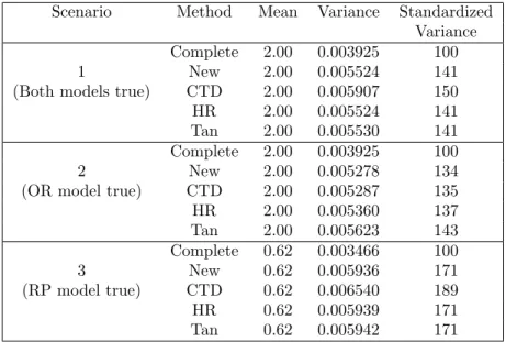
Table 1 presents the Monte Carlo averages and variances of the five esti-mators under the different scenarios. New, HR, CTD, and Tan were all ap-proximately unbiased in all scenarios, illustrating that their double robustness. Turning to relative efficiency, the New estimator showed the best performances in all cases. In Scenario 1, the CTD estimator had the largest variance. In Scenario 2, the New estimator showed the best performance - the calibration condition (5.3) can be justified as the optimality condition when the OR model is true. Tan’s estimator showed slightly higher variance under Scenario 2, whereas the CTD estimator had slightly higher variance under Scenario 3.
Table 1. Monte Carlo average and variance of the point estimators in simu-lation one.
Scenario Method Mean Variance Standardized
Variance
Complete 2.00 0.003925 100
1 New 2.00 0.005524 141
(Both models true) CTD 2.00 0.005907 150
HR 2.00 0.005524 141
Tan 2.00 0.005530 141
Complete 2.00 0.003925 100
2 New 2.00 0.005278 134
(OR model true) CTD 2.00 0.005287 135
HR 2.00 0.005360 137 Tan 2.00 0.005623 143 Complete 0.62 0.003466 100 3 New 0.62 0.005936 171 (RP model true) CTD 0.62 0.006540 189 HR 0.62 0.005939 171 Tan 0.62 0.005942 171
We only consider variance estimation for the CTD method and the New method. The variance estimator proposed by Cao, Tsiatis, and Davidian (2009) was computed using (3.18) with
ηi =m(xi; ˆβ) + δi ˆ pi { yi−m(xi; ˆβ) } −ˆc(δi−pˆi) (1, x2i)′, (5.7)
where ˆβ = ( ˆβ0,βˆ1) and ˆc = (ˆc0,ˆc1) were computed from (5.5). The variance
estimator for the New estimator was computed using (3.18) with ηi=m(xi; ˆβ) + δi ˆ pi { yi−m(xi; ˆβ) } (5.8) and ˆβ= ( ˆβ0,βˆ1) given by (5.4). In (5.8), we obtained ˆpi using maximum
likeli-hood. Variance estimation in the context of Tan’s estimator was not computed here as Tan (2006) did not discuss variance estimation.
Table 2 gives the Monte Carlo bias of the variance estimators and the cov-erage of the interval estimators of the CTD and the New estimators. We used (ˆθ−1.96 √ ˆ V ,θˆ+1.96 √ ˆ
V) for interval estimation. The proposed variance estima-tor for the New estimaestima-tor showed small relative biases (less than 5% in absolute values) in all scenarios, suggesting that the variance estimator for the New es-timator is doubly robust. The variance eses-timator for CTD showed somewhat modest bias (8.27%) under Scenario 3.
Table 2. Monte Carlo percent relative bias of the two variance estimators and coverage of the two interval estimators in simulation one.
Scenario Method Relative Coverage
Bias (%) (%) 1 New 2.27 95.1 CTD 5.75 94.9 2 New 4.69 95.5 CTD 3.33 95.4 3 New -0.04 94.7 CTD 8.27 94.7
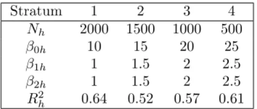
Table 3. Characteristics of the population.
Stratum 1 2 3 4 Nh 2000 1500 1000 500 β0h 10 15 20 25 β1h 1 1.5 2 2.5 β2h 1 1.5 2 2.5 R2 h 0.64 0.52 0.57 0.61
5.2. Survey sampling set-up
We carried out a simulation study in the survey sampling set-up. We gen-erated a population of size N = 5,000 consisting of four strata U1, . . . , U4 of
size N1, . . . , N4, respectively. We generated 5 variables: a variable of interest y
and three auxiliary variables x1-x3. Each of the x-variable was independently
generated from a Gamma distribution with parameters 2 and 25. Then, givenx1
and x2, they-values were generated according to
yi=β0h+β0h+β1hx1i+β2hx2i+ϵi, fori∈Uh,
where theϵi’s were generated from a normal distribution with mean 0 and
vari-anceσh2, i∈Uh,whose value was set to lead to a given coefficient of determination
(R2h). The characteristics of the population are shown in Table 3.
The objective consisted in estimating the finite population mean θN =
n−1∑i∈Uyi. From the population we generated R = 5,000 samples, in each
stratum a simple random samplesh of sizenhwas selected fromUh,h= 1,2,3,4.
Equal allocation was used withnh = 125 andnh= 250, which correspond to an
overall sampling fraction of 10% and 20%, respectively. This particular design leads to unequal probability of selection for units in different strata.
In each selected sample, nonresponse to the study variable y was generated according to
logit (pi) =−2 + 0.03x1i+ 0.03x2i.
We computed five estimators of the mean: the complete sample estimator (C) given by (2.1) with wi = 1/(N πi); the propensity score adjusted (PSA)
estimator given by (2.1) with wi = 1/(N πipˆi); the estimator of Haziza and Rao
(2006) (HR); the estimator of Cao, Tsiatis, and Davidian (2009) (CTD); the proposed estimator (New). We considered three scenarios:
(i) Scenarios 1: The RP and the OR models were correctly specified.
(ii) Scenario 2: Only the OR model was correctly specified. For the RP working model, we used logit(pi) =ϕ0+ϕ1x1i+ϕ2x3i.
(iii) Scenario 3: Only the RP model was correctly specified. For the OR working model, we usedE(yi|xi) =β0+β1x1i+β3x3i.
As a measure of the bias of an estimator ˆθ, we used the Monte Carlo Percent Relative Bias (RB), RB(ˆθ) = 100×EM C(ˆθ)−θN θN , where EM C(ˆθ) = R−1 ∑R
r=1θˆ(r) and ˆθ(r) denotes the estimator ˆθ for the r-th
sample. To compare the efficiency of the estimation procedures, we computed the percent relative efficiency, using the complete sample estimator as the reference. In each sample, we computed the estimator of the total variance (corre-sponding to the New estimator) given by (4.9). In order to compute (4.8), we used ψ(xi; ˆα) = ∑ i∈swiδieˆ2i ∑ i∈swiδi ,
where ˆeidenotes the residual attached to unitiobtained after fitting the working
outcome regression model. As a measure of the bias of ˆVT, we used the Monte
Carlo percent relative bias of the variance estimator. The relative bias of ˆVT is
shown in Table 4 (in parentheses).
Table 4 presents the Monte Carlo percent relative bias and percent relative efficiency (with respect to the complete data estimator) of five estimators under the three scenarios. The HR, CTD, and New estimators all showed negligible bias in all scenarios, which is an indication that they are all doubly robust. The PSA estimator showed a modest bias when the RP model was misspecified. In terms of efficiency, the estimators HR, CTD, and New showed similar performances in all the scenarios, although the CTD was slightly less efficient than the other two. When the RP model was misspecified (Scenario 2), the PSA estimator showed a low efficiency, as expected, and the other two estimators showed almost identical performances. In Table 4, the proposed variance estimator shows good performances in all scenarios (with a relative absolute bias less than 5%).
Table 4. Monte Carlo percent relative bias and percent relative efficiency of five estimators and Monte Carlo percent relative bias of the proposed variance estimator. f = 0.1 f = 0.2 Scenario Method RB RE RB RE Complete 0.00 100 0.00 100 PSA 0.04 271 0.01 278 1 HR 0.04 270 0.01 278 CTD 0.08 274 0.03 281 New 0.04 270 0.01 278 (-1.2) (2.5) Complete 0.00 100 0.00 100 PSA 0.76 394 0.75 550 2 HR 0.03 267 0.01 296 CTD 0.05 270 0.02 298 New 0.03 267 0.01 296 (-1.4) (-3.1) Complete 0.00 100 0.01 100 PSA 0.05 265 0.04 288 3 HR 0.06 264 0.05 289 CTD 0.09 268 0.06 291 New 0.06 264 0.05 288 (3.7) (1.7)
Percent relative biases of the variance estimators are in parenthesis.
6. Concluding remarks
In this paper, we proposed a new doubly robust estimator that showed good finite sample performances in simulation studies. The resulting variance estima-tor is also doubly robust and can be readily implemented using complete data software.
The proposed estimator is based on single deterministic imputation and it is well known that the single imputation of the form (2.3) can lead to biased estimates for the population proportions. In this case, fractional imputation, considered by Fay (1996), Kim and Fuller (2004) and Fuller and Kim (2005), can be used to obtain valid estimates for several parameters. Doubly robust fractional imputation will be discussed elsewhere.
In the simulation studies, the new method showed better efficiency than the other doubly robust estimators in most cases, but there is no guarantee that it is uniformly optimal. Further investigation in this direction is also a topic of future research.
Acknowledgement
We thank professor J. N. K. Rao, three anonymous referees and an Associate Editor for their constructive comments. The research of the first author was partially supported by a Cooperative Agreement between the US Department of Agriculture Natural Resources Conservation Service and Iowa State University. The research of the second author was supported by grants from the Natural Sciences and Engineering Research Council of Canada.
References
Bang, H. and Robins, J. (2005). Doubly robust estimation in missing data and causal inference models.Biometrics 61, 962-973.
Chang, T. and Kott, P. S. (2008). Using calibration weighting to adjust for nonresponse under a plausible model.Biometrika95, 555-571.
Cao, W., Tsiatis, A. A. and Davidian, M. (2009). Improving efficiency and robustness of the doubly robust estimator for a population mean with incomplete data. Biometrika, 96, 723-734.
Cochran, W. G. (1977).Sampling Techniques. Wiley, New York.
Deville, J.-C. (1999). Variance estimation for complex statistics and estimators: linearization and residual techniques.Surv. Methodol.25, 193-203.
Deville, J. C. and S¨arndal, C. E. (1994). Variance estimation for the regression imputed Horvitz-Thompson estimator.J. Official Statist.10, 381-394.
Fay, R. E. (1991). A Design-Based Perspective on Missing Data Variance. Proceedings of the
1991Annual Research Conference, US Bureau of the Census, 429-440.
Fay, R. E. (1996). Alternative paradigms for the analysis of imputed survey data. J. Amer. Statist. Assoc.91, 490-498.
Firth, D. and Bennett, K. E. (1998). Robust models in probability sampling.J. Roy. Statist. Soc. Ser. B 60, 3-21.
Folsom, R. E. (1991). Exponential and logistic weight adjustments for sampling and nonresponse error reduction.Proceedings of the Social Statistics Section, 197-202. American Statistical Association.
Folsom, R. E. and Singh, A. C. (2000). The generalized exponential model for sampling weight calibration for extreme values, nonresponse, and poststratification.Proceedings of the Sur-vey Research Methods Section,596-603. American Statistical Association.
Fuller, W. A. (2009).Sampling Statistics. Wiley, Hoboken, New Jersey.
Fuller, W. A. and Kim, J. K. (2005). Hot deck imputation for the response model, Surv. Methodol.31, 139-149.
Haziza, D. and Rao, J. N. K. (2006). A nonresponse model approach to inference under impu-tation for missing survey data.Surv. Methodol.32, 53-64.
Iannacchione, V. G., Milne, J.G., and Folsom, R.E. (1991). Response probability weight adjust-ments using logistic regression. Proceeding in Survey Research Method Section, 637-642. American Statistical Association.
Kang, J. D. Y. and Schafer, J. L. (2008). Demystifying double robustness: a comparison of alternative strategies for estimating a population mean from incomplete data.Statist. Sci.
Kim, J. K. and Fuller, W. A. (2004). Fractional hot deck imputation.Biometrika 91, 559-578. Kim, J. K. and Kim, J. J. (2007). Nonresponse weighting adjustment using estimated response
probability.Canad. J. Statist.35, 501-514.
Kim, J. K. and Park, H. A. (2006). Imputation using response probability.Canad. J. Statist.
34, 171-182.
Kim, J.K. and Rao, J.N.K. (2009). Unified approach to linearization variance estimation from survey data after imputation for item nonresponse.Biometrika96, 917-932.
Kim, J. K. and Riddles, M. (2012). Some theory for propensity scoring adjustment estimator.
Surv. Methodol.38, 157-165.
Kott, P. S. (1994). A note on handling nonresponse in sample surveys.J. Amer. Statist. Assoc.
89, 693-696.
Kott, P.S. (2006). Using calibration weighting to adjust for nonresponse and coverage errors.
Surv. Methodol.32, 133-142.
Kott, P.S. and Chang, T. (2010). Using calibration weighting to adjust for nonignorable unit nonresponse.J. Amer. Statist. Assoc.105, 1265-1275.
Randles, R. H. (1982). On the asymptotic normality of statistics with estimated parameters.
Ann. Statist.10, 462-474.
Rao, J. N. K. and Shao, J. (1992). Jackknife variance estimation with survey data under hot deck imputation.Biometrika 79, 811-822.
Robins, J. M., Rotnitzky, A. and Zhao, L. P. (1994). Estimation of regression coefficient when some regressors are not always observed.J. Amer. Statist. Assoc.89, 846-866.
Rubin, D. B. (1976). Inference and missing data.Biometrika 63, 581-592.
Rubin, D. B. and van der Laan, M. J. (2008). Empirical efficiency maximization: Improved locally efficient covariate adjustment in randomized experiments and survival analysis.
International Journal of Biostatistics 4.
S¨arndal, C. E. (1992). Method for estimating the precision of survey estimates when imputation has been used.Survey Methodology 18, 241-252.
S¨arndal, C. E., Swensson, B., and Wretman, J. (1992). Model Assisted Survey Sampling.
Springer-Verlag.
Scharfstein, D. O., Rotnitzky, A., and Robins, J. M. (1999). Adjusting for nonignorable drop-out using semiparametric nonresponse models (with discussion and rejoinder). J. Amer. Statist. Assoc.94, 1096-1146.
Shao, J. and Steel, P. (1999). Variance estimation for survey data with composite imputation and nonnegligible sampling fractions.J. Amer. Statist. Assoc.94, 254-265.
Tan, Z. (2006). A distributional approach for causal inference using propensity scores.J. Amer. Statist. Assoc.101, 1619-1637.
Department of Statistics, Iowa State University, Ames, Iowa, 50011, U.S.A. E-mail: [email protected]
D´epartement de math´ematiques et de statistique, Universit´e de Montr´eal, Montreal, H3C 3J7, Canada.
E-mail: [email protected]