Time Series Operators for MonetDB

(1)

Horizon 2020

Understanding Europe’s Fashion Data Universe

Time Series Operators for

MonetDB

Deliverable number: D2.4

Version 3.0

(2)

Project Acronym: FashionBrain

Project Full Title: Understanding Europe’s Fashion Data Universe

Call: H2020-ICT-2016-1

Topic: ICT-14-2016-2017, Big Data PPP: Cross-sectorial and cross-lingual data integration and experimentation

Project URL: https://fashionbrain-project.eu

Deliverable type Other (O) Dissemination level Public (PU) Contractual Delivery Date 31 December 2018 Resubmission Delivery Date 4 February 2019

Number of pages 30, the last one being no. 24

Authors Ying Zhang, Pedro E. S. Ferreira, Svetlin Stalinov, Aris Koning, Martin Kersten - MDBS

Ines Arous, Mourad Khayati - UNIFR

Peer review Tom Oberhauser, Benjamin Winter - BEUTH

Change Log

Version Date Status Partner Remarks

0.1 19/11/2018 Draft MDBS

0.2 15/12/2018 Full Draft MDBS, UNIFR

1.0 20/12/2018 Final MDBS, UNIFR, Rejected 30/01/2019

BEUTH

2.0 04/02/2019 Resubmitted Final MDBS, UNIFR, Rejected 09/03/2020 BEUTH

3.0 15/03/2030 Resubmitted Final 2 MDBS, UNIFR, added URL of RecovDB live demo in Abstract & Introduction

Deliverable Description

D2.4 Time Series Operators for MonetDB (M24). This deliverable will report the extended support for time series data processing in MonetDB, including integration with the software provided by D4.1. Corresponding software will be made available through the MonetDB open-source repository.

(3)

Abstract

In this deliverable, we report the work we have done under the context of T2.3 “infrastructures for scalable cross-domain data integration and management” on the expended support for time series data processing in MonetDB. This include two main topics: RecovDB and SQL 2011 window functions in MonetDB.

RecovDB [1] is an Relational Database Management System (RDBMS) for efficient and accurate recovering of large blocks of missing values in time series. RecovDB is built using MonetDB and the centroid decomposition technology [5]. The live demo of RecovDB is available from http://revival.exascale.info/recovery/ recovdb.php.

To strengthen MonetDB’s support for time series and continues query processing, we have added the majority of the window functions defined by the SQL 2011 standard into MonetDB. In addition, we have rigorously revised the existing code base so that the window functions in MonetDB are now implemented in an efficient way.

(4)

List of Figures

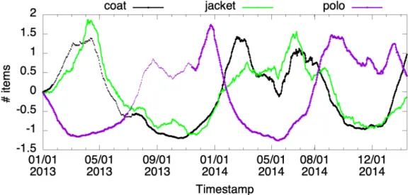
2.1 Zalando sales time series, one for each fashion item. Missing values are indicated by dashed lines. The three time series also show both positive and negative correlations: coats and jackets are more popular in the cold months, which polo’s are more popular in the warm months. 4 2.2 Meteorological time series of temperature and humidity values

measured in Basel, Switzerland during 2017 – 2018. The missing blocks are denoted by dashed lines. . . 7 2.3 RecovDB performance. . . 12 2.4 GUI of the RecovDB demo. . . 13 3.1 Seven days moving average of Zalando sales data gross amount. . . . 21

List of Tables

(6)

List of Acronyms and Abbreviations

CD Centroid Decomposition

DBMS Database Management System

FaBIAM FashionBrain Integrated Architecture

ICDE 2019 35th IEEE International Conference on Data Engineering

OLAP Online Analytical Processing

PCC Pearson Correlation Coefficient

RDBMS Relational Database Management System

RMSE Root-Mean-Square Error

SSV Scalable Sign Vector

(7)

1 Introduction

The FashionBrain project targets at consolidating and extending existing European technologies in the area of database management, data mining, machine learning, image processing, information retrieval, and crowd sourcing to strengthen the positions of European (fashion) retailers among their world-wide competitors. For fashion retailers, the ability to efficiently extract, store, manage and analyse information from heterogeneous data sources, including structured data (e.g. product catalogues and sales information), unstructured data (e.g. twitter, blogs and customer reviews), and binary (multimedia) data (e.g. YouTube and Instagram), is business critical. Therefore, in work package WP2 “Semantic Data Integration for Fashion Industry”, one of the main objectives is to

“Design and deploy novel big data infrastructure to support scalable multi-source data federation, and implement efficient analysis primitives at the core of the data management solution.”

This objective is addressed by task T2.3 “Infrastructures for scalable cross-domain data integration and management”, which focus on the implementation of cross-domain integration facilities to support advanced text and time series analysis. The work we have done in the context of T2.3 is being reported now in two deliverables both due in M24. In the sibling deliverable D2.3 “Data Integration Solution”, we describe the design, implementation and application of FashionBrain Integrated Architecture (FaBIAM), a MonetDB-based architecture for storing, managing and analysing of fashion data.

Time series data are series of values obtained at successive times with regular or irregular intervals between them. Many fashion data, such as customer reviews, fashion blogs, social media messages and click streams, can be regarded as time series. Fashion retailers need efficient, accurate and easy-to-use tools to analyse such fashion time series, so as to understand the current trends, detect changes in the moods and even predict future interests of their (potential) customers. In this deliverable, we present two major extensions in the analytical RDBMS MonetDB1

to facilitate fashion time series analysis:

• R_ecovDB [1]: many fashion time series contains “holes”, because the data records are often produced at irregular time intervals, or because data can get lost for various reasons such as transmission errors. However, existing time series analysis tools, models and algorithms often require perfect input 1

(8)

1. Introduction 1.1. Scope of this Deliverable

time series (i.e. regular time intervals with all values present). Hence, recovering missing values in time series (also often referred to as “missing values imputation”) has become an important prerequisite for time series analysis. Therefore, we have developed R_ecovDB, an RDBMS for efficientand accurate recovering of large blocks of missing values in time series. RecovDB is built using MonetDB and the centroid decomposition technology [5]. This is a joint work between the partners MDBS and UNIFR. This work has been published at 35th IEEE International Conference on Data Engineering (ICDE 2019). The live demo of RecovDB is available fromhttp://revival. exascale.info/recovery/recovdb.php.

• SQL 2011 window functions: to strengthen MonetDB’s support for time series and continues query processing, we have added the majority of the window functions defined by the SQL 2011 standard into MonetDB. In addition, we have rigorously revised the existing code base so that the window functions in MonetDB are now implemented in an efficient way2_.

1.1 Scope of this Deliverable

The work presented here has been guided by the business scenarios identified in D1.2 “Requirement analysis document”, in particular:

• Scenario 3: Brand Monitoring for Internal Stakeholders

– Challenge 7: Online Analytical Processing (OLAP) Queries over Text-and Catalogue Data

• Scenario 4: Fashion Trends Analysis

– Challenge 8: Textual Time Trails

– Challenge 9: Time Series Analysis

The work presented here relates to the following deliverables:

• D1.2 “Requirement analysis document”: in which our motivating fashion time series use cases were defined.

• D2.2 “Requirement analysis document WP2”: in which the Zalando sales data sets used in this deliverable are described.

• D2.3 “Data Integration Solution”: in which the time series operators are used. • D5.4 “The classification algorithm and its evaluation on fashion time series”:

in which Centroid Decomposition (CD) was described.

• D5.5 “Demo on Fashion Trend Prediction”: in which RecovDB will be used. The reminder of this deliverable is as follows. In Chapter 2, we detail the design, implementation and use cases of RecovDB. In Chapter 3, we describe the SQL 2011

2_{Before FashionBrain, MonetDB only supported a small number of window functions implemented}

(9)

1. Introduction 1.1. Scope of this Deliverable

window functions in MonetDB Finally, in Chapter 4 we conclude with outlook for future work.

(10)

2 Time Series Missing Blocks Recovery

Figure 2.1: Zalando sales time series, one for each fashion item. Missing values are indicated by dashed lines. The three time series also show both positive and negative correlations: coats and jackets are more popular in the cold months,

which polo’s are more popular in the warm months.

In its most basic form, a time series is a series of values that have been measured/obtained/generated/etc. at (successive) timestamps with regular or irregular intervals between them. Each value is typically annotated with its corresponding timestamp. In the fashion industry, a large portion of data is time series. For instance, customer reviews, fashion blogs, social media messages and click streams can be all regarded as time series with irregular time intervals1. Since the fashion industry is all about understanding and anticipating what fashion trends the general public is interested at a given time, time series analysis is a particularly important topic for the fashion retailers.

When analysing fashion time series, we should always be prepared to handle missing values, because i) the aforementioned fashion data often come into existence at irregular time intervals; ii) data can get lost for various reasons; and iii) even if we have several perfectly regular time series, they can have different time intervals, which, when aligned by their timestamps, results in missing values. However, many existing tools, algorithms and models for time series analysis assume perfect input time series, i.e. all time series are aligned by their timestamps, the time intervals are

1

(11)

2. Time Series Missing Blocks Recovery

regular and all values at each timestamp are known. Hence, missing values recovery is often the first and a crucial step for time series analysis.

Example 1 (Fashion time series). Consider Zalando apparel sales which are recorded, e.g. on a daily basis as shown in Figure 2.1 (taken from the “Zalando data M3” data sets described in D2.2). The sales numbers of each fashion item is recorded in one time series. There are two main features of interest: i) missing values in the time series; and ii) correlations between the time series. First, fashion supply chains commonly deploy historical sales data gathered from downstream to perform predictions according to which all the upstream activities are planned (e.g., manufacturing scheduling, transportation, inventory and warehouse management). The predictions are pivotal for fashion retailers as they govern the overall revenue generated for all partners within the supply chain. The accuracy of the prediction heavily relies on the use of the complete fashion data. However, due to various reasons, e.g transmission errors or data integration malfunctions,missing values are omnipresent in fashion time series data. For example, in the case of the largest European fashion retailer Zalando, it is not uncommon that around 40% of sales data are missing. Table 2.1 shows an excerpt of Zalando’s sales record shown in Figure 2.1. Each row describes the aggregated number of items sold for three fashion categories during a specific day, and the missing values are marked with the placeholder ‘?’. The values have been normalized using the commonly usedz-score normalization technique.

date coats jacket polo . . . 1 0.054 0.068 ? . . .

2 ? ? ? . . .

3 ? 0.061 ? . . . 4 ? ? 0.047 . . . . . . .

Table 2.1: Fashion sales.

Secondly, fashion sales time series often has seasonal patterns, i.e. items that belong to the same season tend to have similar sales fluctuations. For example, Figure 2.1 shows that coats and jackets are more popular during winter and hence, their sales are positively correlated. However, polo shirts are more popular in the summer and hence, their sales show a negative correlation with the sales of coats and jackets. Thus, a missing value recovery technique should ideally be able to take advantages of such correlations to improve its efficiency and/or accuracy.

Inspired by the use cases of time series data in the FashionBrain project, we have designed and implemented RecovDB, an RDBMS enhanced with advanced matrix decomposition technology for missing blocks recovery. In this chapter, we detail the

(12)

2. Time Series Missing Blocks Recovery 2.1. Design Considerations

main features of R_ecovDB that are important for today’s time series analysis but are lacking in state-of-the-art technologies:

1. Recovering large missing blocks in multiple time series at once;

2. Achieving high recovery accuracy by benefiting from different correlations across time series;

3. Maintaining recovery accuracy under increasing size of missing blocks;

4. Maintaining recovery efficiency with increasing time series’ lengths and the number of time series; and

5. Supporting all these features while being parameter-free.

We also compare the efficiency and accuracy of RecovDB against state-of-the-art missing value recovery systems.

In the remainder of this chapter, we first discuss the state-of-the-art of time series missing value recovery, which has largely determined the design choices of RecovDB. In Section 2.2, we describe the recovery algorithm. In Section 2.3, we describe the implementation of RecovDB. In Section 2.4, we present evaluation results against two state-of-the-art systems on recovery efficiency and accuracy. In Section 2.5, we describe the web application we have been working on, which will be used to visualise the aforementioned main features of RecovDB. This includes three scenarios. Scenario 1 shows that RecovDB can recover multiple time series in one go. Scenario 2 shows that RecovDB maintains the recovery accuracy high when increasing sizes of missing blocks. Scenario 3 shows that even with more and/or longer time series, RecovDB can still recover the missing blocks efficiently. For all three scenarios, one merely needs to select the desired time series and press the “Recover” button, hence no parameter tuning is required. Finally, Section 2.6 concludes.

2.1 Design Considerations

Our work is motivated by the properties of acquired data and the requirements for their subsequent analysis in many real-world use cases. In fact, the missing value and correlation properties we have observed in fashion time series are generally present in other time series as well.

Example 2 (Meteorology time series). Consider the meteorology domain, in which sensors are used to record various weather conditions to perform weather forecast. Figure 2.2 shows three time series containing temperature and humidity values measured in the city of Basel, Switzerland during 2017 – 20182. Next to trends, weather is another important factor that can have significant effect on the fashion sales. For instance, in the Netherlands, unusually warm winter months in recent years have caused consumers to withhold their interests in winter clothes. This

(13)

Figure 2.2: Meteorological time series of temperature and humidity values measured in Basel, Switzerland during 2017 – 2018. The missing blocks are

denoted by dashed lines.

has forced the fashion retailers to put their winter collections back to storage, while refilling their assortments with offerings for warm weather.

When analyzing such meteorological time series, there are a number of important aspects to take into account. First, within the same (scientific) domain, different time series often exhibit some types of correlations. In Figure 2.2, the two temperature time series, “Temp. 2017” and “Temp. 2018”, have a positive correlation with each other, while they both have a negative correlation with the humidity time series “Humidity 2018”. Second, real-world time series often contain a large number of blocks of missing values due to sensor failures, power outages, transmission problems, etc. Some missing blocks can be rather big (shown as dashed lines in Figure 2.2), because, for instance, it can take minutes, hours or even days for a broken sensor to be replaced. Finally, many of the analysis tools and prediction models that meteorologists use to perform weather forecast require complete time series (i.e. the set of the input time series must have the same length, same time interval and all values are known).

In addition, even if a tool can work with incomplete time series, missing values are considered harmful. For instance, missing values often yield incorrect or ill-defined query results [3]. Also, missing values can unexpectedly introduce bias into the time series which might significantly alter their statistical properties, such as the correlations between time series. This in turn can affect further data analysis tasks, e.g. data sampling, exploration and prediction, rendering their results pointless. Given the amount of data we nowadays need to deal with and the requirements of existing models/tools,efficient and accurate recovery of large missing blocks in time series has become a prerequisite to enable the work of many analytical applications.

(14)

Existing recovery techniques have several drawbacks. They either focus on repairing very small missing blocks (i.e., single missing values or only a handful of consecutive missing values) which generally can not yield a high accuracy when applied on big missing blocks [9], or they repair individual time series, while ignoring their correlations with other similar time series [10]. This limits the recovery accuracy, because in many systems today, multiple sensors are used to record the same/similar measurement, which makes using correlation beneficial in many applications such as error detection or missing values recovery.

Moreover, existing techniques are often stand-alone, as opposed to being integrated into a database system. As a result of this, the users of these tools have to conduct a number of time consuming and error-prune tasks themselves, such as either export/import time series from/into a database or do all data management work themselves, repeatedly load the data files and convert them to some internal format, and write code for every action that needs to be conducted on the time series (e.g. filtering and aggregations).

The integration of data mining tasks such as the recovery of missing values in industrial Database Management System (DBMS)s has so far received scant attention. This is mainly because external statistical and data mining tools, such as R3 and WEKA4, offer a comprehensive set of recovery techniques. However, to use these tools, one will have to export time series data already stored in a DBMS into flat files. This approach has a number of serious drawbacks, especially with growing data sizes: i) many of those statistical tools can only operate on data fitting into the main memory; ii) potential performance bottleneck due to data exporting and reloading; iii) loss of data provenance; and iv) losing fundamental DBMS functionality, e.g. query processing, security, concurrency control and fault tolerance) [6].

To overcome the aforementioned problems, we built RecovDB, an RDBMS enhanced with advanced missing blocks recovery technology, which is based on our memory-efficient matrix decomposition technique, the CD [5], to perform scalable and accurate recovery of missing values. The recovery algorithm has been tightly integrated into the open-source analytical RDBMS MonetDB [2] as native User Defined Functions (UDF)s. With this architecture, RecovDB has a number of properties that are highly desirable for missing blocks recovery in large time series, which many of the existing recovery techniques fall short in providing (one or a combination of):

Parameter-free recovery Parametric recovery techniques are based on fine-tuning some input parameters which requires an expertise of the application field and the types of time series. RecovDB avoids parameter tuning by performing recovery based on the centroid value of all time series. The centroid value is the only statistical property we use for the recovery.

3_{https://www.r-project.org}

4

(15)

2. Time Series Missing Blocks Recovery 2.2. RecovDB Recovery Algorithm

Correlation-aware recovery The CD algorithm embeds the correlation across time series yielding a recovery with better performance and higher accuracy.

Large missing blocks in multiple time series By using advanced matrix decom-position technique, RecovDB is capable of accurately recovering multiple time series with large missing blocks in one go, something that cannot be handled well by standard statistical methods such as interpolations.

Full-fledged DBMS support Due to the tight integration, RecovDB can exploit MonetDB’s full power as a highly optimized analytical RDBMS to handle the remaining data management and pre-/post-processing work.

2.2 RecovDB Recovery Algorithm

The recovery algorithm is based on our memory-efficient algorithm to compute the CD for long time series [5]. This section first defines several basic concepts used in CD, before describing the recovery algorithm.

2.2.1 Centroid Decomposition (CD)

LetXbe ann×mmatrix containingmtime series each withnnumerical values. CD decomposesX into ann×mmatrix Land anm×m matrixR so thatX=L·RT, whereRT _{is the transpose of}_R_{. The function}_CD₍_X_{, m}₋_{1) returns the first}_m₋₁

columns ofL and R so that their productXe is an approximation of X.

The most challenging part of computing the CD of X is to find the maximizing sign vector Z, which contains only 1s and −1s, that maximizes the centroid value

kXT_·_Z_k_{, where} _XT _{is the transpose of} _X _and _k·k _{denotes the norm of a vector.}

To efficiently compute Z, we use our Scalable Sign Vector (SSV) algorithm [5], which embeds the correlation across time series without constructing the correlation matrix. The SSV algorithm maintains linear complexity for both time and space with an increasing number of time series.

2.2.2 Recovery Algorithm

Algorithm 1 depicts our recovery algorithm RecovM. It uses CD to recover missing values in multiple time series in one go. RecovM takes as input a matrix X and a list T of pairs indicating the rows and columns of the missing values in X. The recovery starts by initializing the missing values using linear interpolation (line 1). Then, we use SSV to efficiently compute Z (line 2), which is then used to compute the approximated matrix Xe (lines 4-6). Finally, the values in X with positions in

T are updated with their corresponding ones inXe (lines 6-8). The recovery process continues until the Frobenius5 _difference _k_X₋_X0_k

F (as defined by Equation 2.1)

5

(16)

2. Time Series Missing Blocks Recovery 2.3. RecovDB Implementation

Algorithm 1: RecovM(X, T ).

Input :n×m matrix X; List of missing time points T

Output:Matrix with recovered values Xe Linearly interpolate all missing values inX;

Z := SSV(X); repeat X0 :=X; e L,Re := CD(X0,m−1); e X :=Le·ReT;

// Update missing values foreach (i, j)∈T do

xij := ˜xij;

untilkX−X0kF < ;

returnXe;

betweenX and X0 falls below a small threshold (by default 10 5) (lines 3-9).

kX−X0kF = v u u t n X i=1 (xi−x0i)2, where xi ∈X, x0i ∈X0 (2.1)

2.3 RecovDB Implementation

RecovDB is implemented using MonetDB, an open-source RDBMS optimized for in-memory processing of analytical workloads [2]. Internally, MonetDB stores the data of each SQL column as a single C array. This columnar storage model matches nicely with time series data.

CREATE TABLE tss(ts timestamp, v1 float, .., vn float); CREATE FUNCTION recov(ts timestamp, v1 float, .., vn float)

RETURNS TABLE (ts timestamp, f1 float, .., fn float) ...;

SELECT * FROM recov((SELECT ts, v1, v3, v7 FROM tss WHERE ts BETWEEN $TS_MIN AND $TS_MAX));

The SQL queries above show a skeleton of the implementation. First, we store all time series of one data set in a single table6 containing one timestamp column and a number of value columns to hold the values of the time series (after some preprocessing to align the timestamps). Then, we implemented RecovM (see Algorithm 1) and its auxiliary functions as native SQL UDFs in MonetDB7. The

6_{Assuming those time series contain related information, e.g. a weather data set can contain time}

series of temperature and wind speed.

7

(17)

2. Time Series Missing Blocks Recovery 2.4. RecovDB Evaluation

table returning function8 _recov _{is a wrapper for} _RecovM_{. It takes one column of}

timestamps and multiple columns of time series values containingNULLs as missing blocks as its inputs, and passes the value columns to RecovM for imputation. The recovered time series are returned together with the original timestamps in a single table9_{. Finally, we use} _recov _{in a} _SELECT _{query to recover the values of three time}

series within a given time period.

2.4 RecovDB Evaluation

To evaluate the efficiency and accuracy of RecovDB, we have conducted extensive experiments against two state-of-the-art systems in missing value imputation: ImputeDB [3] and BayesDB [8]. We measure i) the runtime to perform the full recovery, and ii) the accuracy of the recovery using the Root-Mean-Square Error (RMSE) between the original block and the recovered one.

We used the BAFU data set provided by the BundesAmt F¨ur Umwelt (the Swiss Federal Office for the Environment)10_{. This data set contains water discharge time}

series of 12 different Swiss rivers recorded every 30 min during 2010 – 2015 resulting in 80k records per time series. The Pearson Correlation Coefficient (PCC)11between these time series range from 0.03 (very low) to 0.89 (quite high), which allows us to evaluate RecovDB for different correlation “strengths”. Each tuple in a time series contains a timestamp and the value of the measurement.

To evaluate the efficiency of RecovDB, we used two set-ups. First, we fixed the length of the 12 time series to 10k, while incrementally dropping 10% of successive values from three different time series (the missing blocks are partially overlapping). Figure 2.3a shows that the runtime of RecovDB is barely sensitive to the percentage of missing values and is up to 5x faster than ImputeDB (0.17sec vs. 1sec) and up to 2900x faster than BayesDB (0.17sec vs. 500sec). Second, we increase the length of all 12 time series from 10k to 80k (Figure 2.3b). Our results show that RecovDB is up to 10x faster than ImputeDB (1.67sec vs 17.77sec), and up to four orders of magnitude faster than BayesDB (0.8sec vs 3343sec).

To evaluate the accuracy of RecovDB, we used the same two set-ups, but measured the RMSEs instead. Figure 2.3c shows that the RMSE of RecovDB is barely affected with more missing values while the RMSE of ImputeDB and BayesDB tends to increase with the percentage of missing values. RecovDB is up to 7.9x more accurate than ImputeDB (0.18 vs. 1.42) and 3.4x more accurate than BayesDB (0.17 vs. 0.57).

Figure 2.3d shows that when increasing the length of time series, RecovDB is up

8_{www.monetdb.org/Documentation/Manuals/SQLreference/Functions}

9_{Passing around (a pointer to) the}_ts _{column is merely an easy way to keep the repaired time}

series annotated with their timestamps. This does not incur additional space and computation.

10_{https://www.bafu.admin.ch/}

11

(18)

2. Time Series Missing Blocks Recovery 2.5. RecovDB Web Interface

(a) Runtime with increasing missing values.

(b) Runtime with increasing time series length.

(c) Accuracy with increasing missing values.

(d) Accuracy with increasing time series length.

Figure 2.3: RecovDB performance.

to 8.3x more accurate than ImputeDB (0.18 vs 1.49) and 4x more accurate than BayesDB (0.25 vs 0.99).

2.5 RecovDB Web Interface

We have been working on a web application, which will be used to show case the main features of RecovDB. Figure 2.4 shows a screenshot of the RecovDB web interface. Above the graph, one can load more data with the “load time series” button. Seven time series were already loaded and each was assigned a different color and is denoted by its name. One can activate/deactivate a time series by clicking on its legend. The values of the three selected time series are visualised in the main graph below. The sliding bar under the main graph shows that we have zoomed in to only view their values in 1985. At the right-side of the GUI, some textual information about the loaded time series is given, followed by some simple options to change the default number of the time series to be repaired, the time series to be used for correlation,

(19)

2. Time Series Missing Blocks Recovery 2.5. RecovDB Web Interface

Swiss rivers discharge

Source: Federal Oﬃce for the Environment FOEN

Unit: m3/s

Recover

Recover time: -

Frobenius distance: -

No. iterations recovery algorithm:

-load time series

Additional missing values 0%

Figure 2.4: GUI of the RecovDB demo.

the recovery threshold (i.e. in Algorithm 1), and the percentage of additional missing values to introduce. By clicking the “Recover” button, one can start the recovery process for the selected time series. Some statistics will be displayed in the text fields under this button. Finally, the recovered time series is visualized in the main window.

2.5.1 Example Data Sets

In addition to the BAFU data set described in Section 2.3, we will provide more data sets.

To evaluate our system on fashion context, we use sales data set provided by Zalando [4]. The fashion data set contains 950 time series with up to 800 normalized observations each ranging from 2013 to 2015 and with a granularity of 1 day. Their PCCs range from −0.8 to 0.93, which allows us to evaluate RecovDB with both positive and negative correlations.

The MeteoSwiss data set, provided by the Swiss Federal Office of Meteorology and Climatology (meteoswiss.admin.ch), has 20 weather time series each containing 200k records measured every 10 min in different Swiss cities. Their PCCs only range from −0.12 to 0.9, but this data set allows us to evaluate RecovDB with fairly long time series.

The Gas concentration data set [7] contains the concentration level of 24 chemical substances each represented as a time series of 4k records measured every 6 hrs. These measurements were collected in a gas delivery platform facility situated at the University of California in San Diego. This data set contains a larger number of negatively correlated time series with PCCs in [−0.75,0.78].

(20)

2. Time Series Missing Blocks Recovery 2.6. Conclusions

2.5.2 Use Cases

This web interface will provide three scenarios to showcase the main properties of RecovDB.

US1: recover multiple time series at once In this use case, one can select multiple time series with different number of missing blocks of different lengths in the time series. The locations of missing blocks across different time series can be distinct or (partially/fully) overlapping. By clicking the Recover button, one can observe that all missing blocks in all time series are repaired in one go. If the missing blocks have been artificially introduced (see US2 below), the web interface will display both the original values and the repaired values so that users can easily compare the quality of the repair.

US2: accurate recovery with increasing missing values In this use case, one can specify a percentage of missing values in a text field. The web interface will remove this percentage of values from the selected range of the selected time series. By clicking the “Recover” button, all time series will be repaired at once. To compare the accuracy of the recovery, the web interface will show the original values in solid lines, and the recovered values in dotted lines. By specifying larger percentages, one shall be able to observe a fairly stable accurate recovery.

US3: efficient recovery with increasing data size In this use case, one can vary the numbers of selected time series and/or the range of the timestamps. For each configuration, the total recovery time will be displayed under the “Recover” button. By increasing the selection, one shall be able to observe that the execution time slightly increases.

2.6 Conclusions

In this chapter, we have presented RecovDB, a parameter free, efficient and accurate missing blocks recovery system for time series based on matrix centroid decomposition and the RDBMS MonetDB. We have described its design considerations, main algorithm, system design and implementation, performance and accuracy evaluation, and the initial version of a web interface to visualise its main features. In the remainder of the FashionBrain project, we will continue improve the implementation of RecovDB under WP5, so that RecovDB can be used to facilitate fashion trends prediction.

(21)

3 MonetDB Window Function Extensions

To increase MonetDB’s ability to process time series data, We have extended MonetDB’s support for the SQL window functions to cover the majority as specified by the 2011 revision of the SQL standard1 _{in the context of T2.3. In this chapter, we}

elaborate the functionality that has been added together with some example queries to show their usage.

3.1 Feature Extensions

In this section we give specifications of the new window functions.

3.1.1 Window Analytic Functions

Besides the existing RANK(), DENSE RANK() and ROW NUMBER() functions, we have implemented all the remaining analytic functions listed in the SQL standard:

• PERCENT RANK():DOUBLE - calculates the relative rank of the current row, i.e. (rank() - 1) / (rows in partition - 1).

• CUME DIST():DOUBLE- calculates the cumulative distribution, i.e. the number of rows preceding or peer with current row / rows in partition.

• NTILE(nbuckets BIGINT):BIGINT- enumerates rows from 1 in each partition, dividing it in the most equal way possible.

• LAG(input A[, offset BIGINT[, default value A ]]):A - returns input value at row offset before the current row in the partition. If the offset row does not exist, then the default value is output. By defaultoffset is 1 and default value isNULL.

• LEAD(input A[, offset BIGINT[, default value A ]]):A - Returns in-put value at row offset after the current row in the partition. If the offset row does not exist, then the default value is output. By default offset is 1 and default value is NULL.

• FIRST VALUE(input A):A - Returns input value at first row of the window frame.

• LAST VALUE(input A):A - Returns input value at last row of the window frame.

1_{https://sigmodrecord.org/publications/sigmodRecord/1203/pdfs/10.industry.zemke.}

(22)

3. MonetDB Window Function Extensions 3.1. Feature Extensions

• NTH VALUE(input A, nth BIGINT):A- Returns input value at nthrow of the window frame. If there is no nth row in the window frame, then NULL is returned.

3.1.2 Aggregate Functions

We have extended our existing aggregate functions to support aggregate window functions: • MIN(input A) : A • MAX(input A) : A • COUNT(*) : BIGINT • COUNT(input A) : BIGINT • SUM(input A) : A • PROD(input A) : A • AVG(input A) : DOUBLE

3.1.3 Window Functions Frames

Our window functions now support frame specifications from the SQL standard. The fully implemented SQL grammar is listed bellow:

window_function_call:

{ window_aggregate_function | window_rank_function } OVER { ident | ‘(’ window_specification ‘)’ } window_aggregate_function: AVG ‘(’ query_expression ‘)’ | COUNT ‘(’ { ‘*’ | query_expression } ‘)’ | MAX ‘(’ query_expression ‘)’ | MIN ‘(’ query_expression ‘)’ | PROD ‘(’ query_expression ‘)’ | SUM ‘(’ query_expression ‘)’ window_rank_function: CUME_DIST ‘(’ ‘)’ | DENSE_RANK ‘(’ ‘)’ | FIRST_VALUE ‘(’ query_expression ‘)’

| LAG ‘(’ query_expression [ ‘,’ query_expression [ ‘,’ query_expression ] ] ‘)’ | LAST_VALUE ‘(’ query_expression ‘)’

| LEAD ‘(’ query_expression [ ‘,’ query_expression [ ‘,’ query_expression ] ] ‘)’ | NTH_VALUE ‘(’ query_expression ‘,’ query_expression ‘)’

| NTILE ‘(’ query_expression ‘)’ | PERCENT_RANK ‘(’ ‘)’

| RANK ‘(’ ‘)’ | ROW_NUMBER ‘(’ ‘)’ window_specification:

[ ident ] [ PARTITION BY column_ref [ ‘,’ ... ] ] [ ORDER BY sort_spec ]

[ { ROWS | RANGE | GROUPS } { window_frame_start | BETWEEN window_bound AND window_bound } [ EXCLUDING { CURRENT ROW | GROUP | TIES | NO OTHERS } ] ]

window_bound:

UNBOUNDED FOLLOWING | query_expression FOLLOWING

(23)

The supported frames are: ROWS, RANGE and GROUPS.

• ROWS - frames are calculated on physical offsets of input rows.

• RANGE- result frames are calculated on value differences from input rows (used with a custom PRECEDING orFOLLOWING bound requires anORDER BY clause). • GROUPS- groups of equal row values are used to calculate result frames (requires

an ORDER BY clause).

After a window frame declaration, the window bounds must be specified (the window function will be applied to each frame derived from each row in the input). If window frame start bound is provided, then the frame’s end will be set to CURRENT ROW. An UNBOUNDED PRECEDING bound means the first row of a partition, while an UNBOUNDED FOLLOWING means the last row of a partition. In query expression PRECEDING (i.e. frame rows before the current row) and query expression FOLLOWING (i.e. frame rows after the current row) bounds, the query expression can evaluate to a single atom (use the same bound for every input row), or a column (use a different bound for each input row). In either case, everyquery expressionvalue must be non-negative and non-NULL, as negative and NULLbounds are not defined for SQL window functions. CURRENT ROW is equivalent to0 PRECEDING and 0 FOLLOWING on either side of the bound.

The SQL standard allows an EXCLUDING clause after the bounds definition. At the moment only EXCLUDE NO OTHERS (i.e. default one) is implemented, which means all rows in the window frame are used for computation of the analytic function. The frame specification has been implemented for aggregation functions, as well as the functions FIRST VALUE, LAST VALUE and NTH VALUE. The default frame specification is RANGE BETWEEN UNBOUNDED PRECEDING AND CURRENT ROW when there is anORDER BYclause, andRANGE BETWEEN UNBOUNDED PRECEDING AND UNBOUNDED FOLLOWING when an ORDER BY clause is not present.

3.2 Example Queries

In this section, we use several example SQL queries to show how to use some of the new window functions.

CREATE TABLE analytics (col1 int, col2 int); INSERT INTO analytics VALUES

(15, 3), (3, 1), (2, 1), (5, 3), (NULL, 2), ( 3, 2), (4, 1), (6, 3), (8, 2), (NULL, 4);

(24)

3. MonetDB Window Function Extensions 3.2. Example Queries

SELECT PERCENT_RANK() OVER (ORDER BY col1) FROM analytics; +---+ | L4 | +====================+ | 0 | | 0 | | 0.2222222222222222 | | 0.3333333333333333 | | 0.3333333333333333 | | 0.5555555555555556 | | 0.6666666666666666 | | 0.7777777777777778 | | 0.8888888888888888 | | 1 | +---+

SELECT FIRST_VALUE(col1) OVER (PARTITION BY col2) FROM analytics; +---+ | L4 | +======+ | 3 | | 3 | | 3 | | null | | null | | null | | 15 | | 15 | | 15 | | null | +---+

SELECT COUNT(col1) OVER (ORDER BY col2 DESC RANGE UNBOUNDED PRECEDING) FROM analytics; +---+ | L4 | +======+ | 0 | | 3 | | 3 | | 3 | | 5 | | 5 | | 5 | | 8 | | 8 | | 8 | +---+

SELECT AVG(col1) OVER (ORDER BY col2 GROUPS BETWEEN UNBOUNDED PRECEDING AND CURRENT ROW) FROM analytics; +---+ | L4 | +======+ | 3 | | 3 | | 3 | | 4 | | 4 | | 4 | | 5.75 | | 5.75 | | 5.75 | | 5.75 | +---+

(25)

We have also implemented interval boundaries for time columns on RANGE frames.

CREATE TABLE timetable (col1 timestamp, col2 int); INSERT INTO timetable VALUES

(’2017-01-01’, 3), (’2017-02-02’, 1), (’2017-03-03’, 1), (’2017-04-04’, 3), (NULL, 2), (’2017-06-06’, 2), (’2017-07-07’, 1), (’2017-08-08’, 3), (’2017-09-09’, 2), (NULL, 4);

SELECT SUM(col2) OVER (ORDER BY col1 RANGE BETWEEN

INTERVAL ’1’ MONTH PRECEDING AND INTERVAL ’3’ MONTH FOLLOWING) FROM timetable; +---+ | L4 | +======+ | 6 | | 6 | | 5 | | 5 | | 5 | | 5 | | 6 | | 6 | | 5 | | 2 | +---+

New WINDOW Keyword. For convenience, we have added support for the WINDOW keyword. If the same window specification is to be used multiple times in aSELECT clause, one can define an alias for this window specification, so as to avoid repeating the same window definition. Such aliases can be defined using the new WINDOW keyword in a FROM clause. In the query below, the definitions of the aliases w1 and w2 show how different aliases can be defined for different window specifications on one table. The definition of the alias w3 shows that different aliases can be defined for the same window specification. Finally, all aliases can be subsequently used in the SELECT clause.

SELECT COUNT(*) OVER w1, PROD(col1) OVER w2, SUM(col1) OVER w1, AVG(col2) OVER w2, MAX(col2) OVER w3

FROM analytics WINDOW

w1 AS (ROWS BETWEEN 5 PRECEDING AND 0 FOLLOWING),

w2 AS (RANGE BETWEEN CURRENT ROW AND UNBOUNDED FOLLOWING), w3 AS (w2); +---+---+---+---+---+ | L4 | L10 | L14 | L20 | L24 | +======+========+======+==========================+======+ | 1 | 259200 | 15 | 2.2 | 4 | | 2 | 259200 | 18 | 2.2 | 4 | | 3 | 259200 | 20 | 2.2 | 4 | | 4 | 259200 | 25 | 2.2 | 4 | | 5 | 259200 | 25 | 2.2 | 4 | | 6 | 259200 | 28 | 2.2 | 4 | | 6 | 259200 | 17 | 2.2 | 4 | | 6 | 259200 | 20 | 2.2 | 4 | | 6 | 259200 | 26 | 2.2 | 4 | | 6 | 259200 | 21 | 2.2 | 4 | +---+---+---+---+---+

Partition Orders. Our previous partitioning implementation did not impose order in the input. With the new implementation of window functions, partitioning now imposes ascending order by default, thus pairing with the industry standard

(26)

implementation. If the same expression occurs in bothPARTITIONandORDERclause, then ORDER defines the input order:

CREATE TABLE ranktest (id INT, k STRING);

INSERT INTO ranktest VALUES (1061,’a’),(1062,’b’),(1062,’c’),(1061,’d’); SELECT ROW_NUMBER() OVER (PARTITION BY id), id FROM ranktest;

-- Output before +---+---+ | L4 | id | +======+======+ | 1 | 1062 | | 2 | 1062 | | 1 | 1061 | | 2 | 1061 | +---+---+ -- Output now +---+---+ | L4 | id | +======+======+ | 1 | 1061 | | 2 | 1061 | | 1 | 1062 | | 2 | 1062 | +---+---+

Fashion sales moving average Moving average2 _{is an important calculation in}

statistics. For example, it is often used in technical analysis of sales data. With the SQL 2011 window functions, it is now much easier to computing statistic methods like moving averages that explicitly address the values by their position in SQL3_.

In this example, we show how to compute moving average for some Zalando sales data [4]. First, we load the data set, which contains among others a gross amount for each day:

sql>CREATE TABLE region1_orders ( more> region INT DEFAULT 1, more> id INT,

more> no_items FLOAT, more> no_orders FLOAT, more> gross_amount FLOAT, more> "date" DATE

more>);

operation successful sql>COPY OFFSET 2 INTO more> region1_orders

more> FROM ’<path-to>/ZALANDO_data_M3/region1_orders.csv’ more> (id, no_items, no_orders, gross_amount, "date") more> DELIMITERS ’,’,’\n’ NULL AS ’’ BEST EFFORT; 729 affected rows

The query below computes moving averages of 7 preceding days for the gross amount.

2_{https://en.wikipedia.org/wiki/Moving_average}

3_{The relational model does not have the notion of order, so table records can only be addressed}

by their combined distinct values. If two records happen to contain exactly the same values, there is no way to distinguish them.

(27)

sql>SELECT "date", gross_amount, AVG(gross_amount) OVER (ORDER BY "date" ASC

more> RANGE BETWEEN INTERVAL ’7’ DAY PRECEDING AND INTERVAL ’0’ DAY FOLLOWING) AS ma1week more> FROM region1_orders;

+---+---+---+

| date | gross_amount | ma1week |

+============+==========================+==========================+ | 2013-03-02 | 0.913448169706 | 0.913448169706 | | 2013-03-03 | 0.900760559146 | 0.907104364426 | | 2013-03-04 | 0.696187810056 | 0.8367988463026667 | | 2013-03-05 | 0.711312403182 | 0.8054272355225 | ... | 2015-02-24 | 1.1476541021 | 1.34353897110375 | | 2015-02-25 | 1.12662334926 | 1.33628887056875 | | 2015-02-26 | 1.05794838226 | 1.3152827855675 | | 2015-02-27 | 1.11077032663 | 1.3009447468287498 | | 2015-02-28 | 1.04995952798 | 1.2978170778875 | +---+---+---+ 729 tuples

The complete result set is best view in a plot as shown in Figure 3.1.

(28)

4 Conclusions

In this document, we have presented two major MonetDB extension to facilitate fashion time series data processing: RecovDB and SQL 2011 window functions. For RecovDB, we have submitted a paper to ICDE 2019 to demonstrate its main features; while the window functions will be released with the coming MonetDB feature release in Q1/2019.

In the remainder of the FashionBrain project, we plan to continue working on both topics:

• Extend the recovery algorithm of RecovDB to handle streaming data (this work is led by UNIFR).

• Porting the RecovDB SQL Python UDF to MonetDB’s native C-UDF for better performance (this is joint work of MDBS and UNIFR).

• Finish the development of the RecovDB demonstration (this is joint work of MDBS and UNIFR).

• Hardening the window function implementation to be release ready (this work is led by MDBS).

(29)

Bibliography

[1] Ines Arous, Mourad Khayati, Philippe Cudr´e-Mauroux, Ying Zhang, Martin Kersten, and Svetlin Stalinlov. RecoveDB: accurate and efficient missing blocks recovery for large time series. In Proceedings of the 35th IEEE International Conference on Data Engineering (ICDE 2019), April 2019.

[2] Peter A. Boncz, Martin L. Kersten, and Stefan Manegold. Breaking the memory wall in MonetDB. Commun. ACM, 51(12):77–85, 2008.

[3] Jose Cambronero, John Feser, Micah Smith, and Samuel Madden. Query optimization for dynamic imputation. PVLDB, 10(11):1310–1321, 2017. URL http://www.vldb.org/pvldb/vol10/p1310-feser.pdf.

[4] FashionBrain. Deliverable D.2.2, Requirement analysis document WP2, August 2017.

[5] Mourad Khayati, Michael H. B¨ohlen, and Johann Gamper. Memory-efficient centroid decomposition for long time series. In IEEE 30th International Conference on Data Engineering, Chicago, ICDE 2014, IL, USA, March 31 - April 4, 2014, pages 100–111, April 2014. doi: 10.1109/ICDE.2014.6816643. URL https://doi.org/10.1109/ICDE.2014.6816643.

[6] Carlos Ordonez and Sasi K. Pitchaimalai. One-pass data mining algorithms in a DBMS with udfs. In Proceedings of the ACM SIGMOD International Conference on Management of Data, SIGMOD 2011, Athens, Greece, June 12-16, 2011, pages 1217–1220, 2011. doi: 10.1145/1989323.1989458. URL http://doi.acm.org/10.1145/1989323.1989458.

[7] Irene Rodriguez-Lujan, Jordi Fonollosa, Alexander Vergara, Margie Homer, and Ramon Huerta. On the calibration of sensor arrays for pattern recognition using the minimal number of experiments. Chemometrics and Intelligent Laboratory Systems, 130:123 – 134, 2014. ISSN 0169-7439.

[8] Feras Saad and Vikash K Mansinghka. A probabilistic programming approach to probabilistic data analysis. InNIPS, pages 2011–2019, 2016.

[9] Jimeng Sun, Spiros Papadimitriou, and Christos Faloutsos. Online latent variable detection in sensor networks. InProceedings of the 21st International Conference on Data Engineering, ICDE 2005, 5-8 April 2005, Tokyo, Japan, pages 1126–1127, April 2005. doi: 10.1109/ICDE.2005.100.

[10] Kevin Wellenzohn, Michael H. B¨ohlen, Anton Dign¨os, Johann Gamper, and Hannes Mitterer. Continuous imputation of missing values in streams of pattern-determining time series. In Proceedings of the 20th International

(30)

BIBLIOGRAPHY BIBLIOGRAPHY

Conference on Extending Database Technology, EDBT 2017, Venice, Italy, March 21-24, 2017., pages 330–341, March 2017.

Time Series Operators for MonetDB

Understanding Europe’s Fashion Data Universe