On OBDDs for CNFs of Bounded Treewidth
Igor Razgon
Department of Computer Science and Information Systems Birkbeck University of London
igor@dcs.bbk.ac.uk
Abstract
In this paper we show that a CNF cannot be compiled into an Ordered Binary Decision Diagram (OBDD) of fixed-parameter size fixed-parameterized by the primal graph treewidth of the CNF. Thus we provide a parameterized separation be-tween OBDDs and Sentential Decision Diagrams for which such fixed-parameter compilation is possible. We also show that the best existing parameterized upper bound for OBDDs in fact holds for incidence graph treewidth parameterization.
Introduction
Knowledge compilation is a rewriting approach to proposi-tional knowledge representation. The ‘knowledge base’ is initially represented as aCNFor even as a Boolean circuit. For these representations many important types of queries areNP-hard to answer. Therefore, the initial representation is compiled into another one for which the minimal require-ment is that the clausal entailrequire-ment query (can the given par-tial assignment be extended to a complete satisfying assign-ment?) can be answered in a polynomial time (Darwiche and Marquis 2002). Such transformation can result in expo-nential blow up of the representation size. A possible way to circumvent this issue is to identify a structural parame-ter of the inputCNFsuch that the resulting transformation is exponential in this parameter and polynomial in the number of variables. A notable result in this direction is anO(2kn) upper bound on the size of Decomposable Negation Nor-mal Form (DNNF) (Darwiche 2001), where n is the num-ber of variables of the givenCNFandkis the treewidth of its primal graph. Quite recently, the same upper bound has been shown to hold for Sentential Decision Diagrams (SDD) (Darwiche 2011), a subclass ofDNNFthat can be seen as a generalization of the famous Ordered Binary Decision Dia-grams (OBDD) and shares with theOBDDthe key nice fea-tures (e.g. poly-time equivalence testing). It is known that aCNFof treewidthkcan be compiled into anOBDDof size
O(nk)(Ferrara, Pan, and Vardi 2005). A natural question is whetherOBDD, similarly toSDD, admits a ‘fixed-parameter’ upper bound of formf(k)ncfor some constantc.
In this paper we provide a negative answer to this ques-tion. In particular, we demonstrate an infinite class ofCNFs Copyright c2014, Association for the Advancement of Artificial Intelligence (www.aaai.org). All rights reserved.
of the primal graph treewidth at mostkfor which theOBDD
size is at leastf(k)nk/4wheref is a function exponentially small ink. In other words, we show that theOBDDsize of these CNFs is Ω(nk/4)for every fixedk. This result
pro-vides a separation fromSDDand essentially matches the up-per bound of (Ferrara, Pan, and Vardi 2005). In fact, this result shows impossibility of not only a fixed-parameter up-per bound, but also of a sublinear dependence on kin the base of the exponent or even of an exponentk/C for some large constantC.
Our second result is ‘strengthening’ of the upper bound
O(nk)of (Ferrara, Pan, and Vardi 2005) by showing that it holds ifkis the treewidth of theincidencegraph of the given
CNFthus extending the upper bound to the case of sparse CNFs with large clauses.
In order to obtain the lower bound, we introduce a no-tion ofmatching widthof a graph and prove that if a CNF F of the considered class has matching widthrof the pri-mal graph then for any ordering of the variables ofF there is a prefixSsuch that the number of distinct functions that can be obtained fromF by assigning the variables ofSis at least2r. This will immediately imply that anyOBDD realiz-ingF will have at least2rnodes. Finally we will prove that the matching width of the consideredCNFs isΩ(logn∗k). Substituting this lower bound insteadrwill get the desired lower bound for theOBDDsize.
Similarly to the case of primal graph, the upper bound is obtained by showing that ifpathwidthof the incidence graph of the givenCNFis at mostpthen thisCNFcan be compiled into anOBDDof sizeO(2pn). Then theO(nk)upper bound is obtained using a well known relation p = O(k∗logn)
between the treewidth and the pathwidth of the given graph. The approach to obtain theO(2pn)bound is similar to (Fer-rara, Pan, and Vardi 2005): variables are ordered ’along’ the path decomposition and it is observed that the for each prefix the number of functions caused by assigning the ’previous’ variables isO(2p). The technical difference is that in our case the bags of the path decomposition include clauses and this circumstance must be taken into account.
The proposed results contribute to a large body of exist-ing results concernexist-ing the space complexity ofOBDDs. To begin with, there are many results concerning the complex-ity of OBDDs forparticular classes of Boolean functions, see e.g. the book (Wegener 2000) and the survey (Wegener
2004). The space complexity of OBDD remains polyno-mial if parameterized by the treewidth of acircuit represent-ing the given function (Jha and Suciu 2012), however the dependence on the treewidth becomes double exponential. A fixed-parameter upper bound can be achieved if tree of
OBDDs is used instead of a single OBDD(McMillan 1994; Subbarayan, Bordeaux, and Hamadi 2007). In the complex-ity theory theOBDDis classified as theoblivious read-once branching program, see the book (Jukna 2012) for the re-sults concerning the complexity of branching programs on particular classes of formulas
The proposed lower bound also contributes to the under-standing of relationship betweenOBDDandSDD. Other re-sults in this direction are (Xue, Choi, and Darwiche 2012) showing an exponential separation betweenSDDandOBDD
based on the same order of variables (the order of variables forSDDis defined as the order of visiting the corresponding nodes of the underlyingvtreeby a left-right tree traversal al-gorithm) and (Choi and Darwiche 2013) empirically show-ing that conceptually similar heuristics produceSDDs orders of magnitude smaller thanOBDDs.
The rest of the paper is structured as follows. The next section introduces the necessary background. The section after that proves the lower bound, the proofs of auxiliary statements are provided in the two following sections. Then follows the section presenting the upper bound for the pa-rameterization by the treewidth of the incidence graph. The last section outlines relevant directions of further research.
Preliminaries
The structure of this section is the following. First, we in-troduce notational conventions. Then we define theOBDD
and specify the approach we use to prove the lower bound. Next, we introduce terminology related toCNFs. Finally, we define the notion of treewidth.
In this paper by aset of literalswe mean one that does not contain an occurrence of a variable and its negation. For a setS of literals we denote byV ar(S)the set of variables whose literals occur inS. IfF is a Boolean function or its representation by a CNF or OBDD, we denote byV ar(F)
the set of variables ofF. A truth assignment toV ar(F)on whichF is true is called asatisfying assignmentof F. A setS of literals represents the truth assignment toV ar(S)
where variables occurring positively inS(i.e. whose literals inS are positive) are assigned withtrueand the variables occurring negatively are assigned withf alse. We denote by
FS a function whose set of satisfying assignments consists ofS0such thatS∪S0is a satisfying assignment ofF. We call
FS asubfunctionofF. In other words, a Boolean function
F0 is a subfunction of a Boolean functionF isF0 can be obtained fromF by giving a truth assignment to a subset of variables ofF.
An OBDDZ representing a Boolean functionF is a di-rected acyclic graph (DAG) with one root and two leaves la-belled bytrueandf alse. The internal nodes are labelled with variables of F. There is a fixed permutation SV of
V ar(F)(that is, elements of V ar(F)are linearly ordered according toSV) so that the vertices along any path from the root to a leaf are labelled with variables according to
this order. Each internal vertex is associated with2leaving edges labelled withtrueandf alse. Each pathP from the root ofZ is called acomputational path and is associated with truth assignment to the variables labelling all the ver-tices but the last one. In particular, each variable is assigned with the value labelling the edge of the path that leaves the corresponding vertex. We denote byA(P)the assignment associated with the computational path P. The set of all
A(P)whereP is a computational path ending at thetrue
leaf is precisely the set of satisfying assignments ofF.
X2 X3 X4 T F T T T T F F F F X1
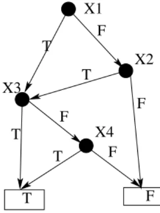
Figure 1: AnOBDDfor(x1∨x2)∧(x3∨x4)under
permu-tation(x1, x2, x3, x4)
Figure 1 shows an OBDD for the function(x1∨x2)∧
(x3∨x4)under the permutation(x1, x2, x3, x4). Consider
the pathP = (x1, x2, x3). ThenA(P) ={¬x1, x2}.
In order to obtain the lower bound on theOBDDsize we use a standard approach of counting subfunctions. See (We-gener 2000) for examples of application of this approach. This approach is based on the following statement.
Proposition 1 LetF be a Boolean function on a setV of variables and letSV be a permutation ofV. PartitionSV into a prefixSV1and a suffixSV2and suppose that the
num-ber of distinct subfunctions ofFobtained by giving truth as-signments to all the variables ofSV1is at leastx. Then an
OBDDofF with the underlying orderSV contains at least xnodes.
The standard way to utilize Proposition 1 is to show that foranypermutationSV ofV there is a partition ofSV into a prefixSV1 and a suffixSV2such that the instantiation of
variables ofSV1results in at leastxdifferent subfunctions.
Then Proposition 1 immediately implies that xis a lower bound on the size ofOBDDforanyunderlying order.
Given aCNF F, its primal graphhas the set of vertices corresponding to the variables of F. Two vertices are ad-jacent if and only if there is a clause of F where the cor-responding variables both occur. In theincidence graphof
F the vertices are partitioned into those corresponding to the variables ofF and those corresponding to its clauses. A variable vertex is adjacent to a clause vertex if and only if the corresponding variable occurs in the corresponding clause.
Given a graphG, itstree decompositionis a pair(T,B)
to the verticestofT. EachB(t)is a subset ofV(G)and the bags obey the rules ofunion(that is, S
t∈V(T)B(t) =
V(G)),containment(that is, for each{u, v} ∈E(G)there ist ∈ V(t)such that{u, v} ⊆ B(t)), andconnectedness (that is for eachu ∈ V(G), the set of alltsuch that u ∈ B(t) induces a subtree ofT). Thewidthof (T,B)is the size of the largest bag minus one. The treewidth ofGis the smallest width of a tree decomposition ofG. IfT is a path then we use the respective notions of path decomposition andpathwidth. V1 V1V2 V1V3 V1 V2 V3 V2 V3 V4 V5 V6 V7 V1 V4 V2 V1 V3 V5 V7 V6
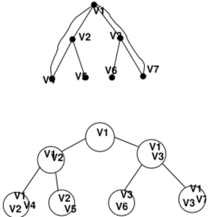
Figure 2: A graph and its tree decomposition Figure 2 shows a graph and its tree decomposition. The width of this tree decomposition is 2since the size of the largest bag is3.
The lower bound
In this section, given two integersrandkwe define a class ofCNFs, roughly speaking, based on complete binary trees of heightrwhere each node is associated with a clique of sizek. Then we prove that the treewidth of the primal graphs of CNFs of this class is linearly bounded byk. Further on, we state the main technical theorem (proven in the next sec-tion) that claims that the smallestOBDDsize forCNFs of this class exponentially depends onrk. Finally, we re-interpret this lower bound in terms of the number of variables and the treewidth to get the lower bound announced in the Introduc-tion.
Let G be a graph. A graph based CNF denoted by
CN F(G)is defined as follows. The set of variables con-sists of variables Xu for each u ∈ V(G) and variables
Xu,v =Xv,ufor each{u, v} ∈ E(G). The set of clauses consists of clauses Cu,v = Cv,u = (Xu ∨Xu,v∨Xv) for each{u, v} ∈ E(G). In other words, the variables of
CN F(G)correspond to the vertices and edges of G. The clauses correspond to the edges ofG.
Denote by Tr a complete binary tree of height r. Let
CTr,k be the graph obtained from Tr by associating each vertex with a clique of sizekand, for each edge{u, v}ofG, making all the vertices of the cliques associated withuand
vmutually adjacent. DenoteCN F(CTr,k)byFr,k. Figure 3 showsT2andCT2,3. To avoid shading the
pic-ture ofCT2,3with many edges, the cliques corresponding to
Figure 3:T2andCT2,3
the vertices ofT2are marked by circles and the bold edges
between the circles mean that that there are edges between all pairs of vertices of the corresponding cliques.
Lemma 1 The treewidth of the primal graph ofFr,k is at leastk−1at most2k−1. In fact, forr≥1, this treewidth is exactly2k−1.
Proof. The primal graph of Fr,k can be obtained from
CTr,kby adding one vertexvefor each edgeeofCTr,kand making this vertex adjacent to the ends ofe.
The lower bound follows from existence of a clique of sizekinCTr,k. Indeed, in any tree decomposition ofCTr,k, there is a bag containing all the vertices of such a clique (Bodlaender and M¨ohring 1993). Consequently, the width of any tree decomposition is at leastk−1. In fact ifr≥1
thenCTr,khas a clique of size2kcreated by cliques of two adjacent nodes. Hence, due to the same argumentation, the treewidth ofCTr,kis at least2k−1forr≥1.
For the upper bound, consider the following tree decom-position (T,B)of CTr,k. T is justTr. We look uponTr as a rooted tree, the centre ofTr being the root. The bag
B(u)of each node ucontains the clique of CTr,k corre-sponding tou. In addition, ifuis not the root vertex then
B(u)also contains the clique corresponding to the parent of
u. Observe that(T,B)satisfies the connectivity property. Indeed, each vertex appears in the bag corresponding to its ‘own’ clique and the cliques of its children. Clearly, the set of nodes corresponding to the bags induce a connected sub-graph. The rest of the tree decomposition properties can be verified straightforwardly. We conclude that (T,B)is in-deed a tree decomposition ofCTr,k.
In order to ‘upgrade’(T,B), add k2
new adjacent ver-tices to each vertex ofT. These vertices will correspond to the edges of cliques associated with the respective nodes of
Tr. In addition, addk2 new adjacent vertices to each non-root vertex ofT. These vertices will correspond to the edges between the clique associated with the corresponding node ofTrand the clique of its parent. The bag of each new ver-tex will containve, corresponding to the edgeeassociated with this bag, plus the ends ofe. A direct inspection shows that this is indeed a tree decomposition of the primal graph ofFr,kand that the size of each bag is at most2k.
Notice that forr ≥ 1the lower and upper bounds coin-cide, thus allowing to state the treewidth precisely.
The following is the main technical result whose proof is given in the next section.
Theorem 1 The size of OBDD computing Fr,k is at least
2rk/2.
Let us reformulate the statement of Theorem 1 in terms of the number of variables ofFr,k and the treewidth of its primal graph, having in mind the bounds on the treewidth as in Lemma 1.
First of all, taking into account that k ≥ p/2, where
p is the treewidth of the primal graph ofFr,k, the lower bound can be seen as 2rp/4. Next, let m be the number
of variables of Fr,k. Then, it is not hard to observe that
2r ≥ m 2(k 2) ≥ m 2((p+1) 2 )
. Replacing 2r this way in 2rp/4,
we obtain( m 2((p+1) 2 ) )p/4 = 2(p+1) 2 −p/4 ∗mp/4as a lower
bound on theOBDDsize forFr,k. Clearly, if we considerp
as a constant, this lower bound can be seen asΩ(mp/4).
Now we are ready to state the main result.
Corollary 1 There is a functionf such that for eachp≥1 there is an infinite sequence ofCNFsF1, F2. . . ,of treewidth
at mostpof their primal graphs such that for eachFi the size ofOBDDcomputing it is at leastf(p)∗mp/4wherem
is the number of variables ofFi. Put it differently, for each fixedp, there is a class ofCNFs of treewidth at mostpof the primal graph for which theOBDDsize isΩ(mp/4).
Proof. For an odd p, consider the CNFs Fr,(p+1)/2 for
allr≥1and for an evenp, consider theCNFsFr,p/2for all
r≥1. Observe that for an evenpthe primal graph treewidth ofFr,pisp−1and that the above argumentation still applies. Indeed, sincek=p/2, it is legitimate to represent the lower bound as2rp/4. Further on, in the inequality that follows, the occurrence ofp+ 1in the denominator (as an upper bound of the actual treewidth) even strengthens this inequality.
Proof of Theorem 1
The plan of the proof is the following. We introduce the notion of matching width of a graph. Then we provide two statements regarding this notion. The first statement (Lemma 2) claims a linear inrklower bound for the match-ing width of graphsCTr,k underlying the considered class
Fr,k (the proof of the lemma is provided in the next sec-tion). The second statement (Lemma 3) claims that if a graphGhas a matching widthtthen any permutation of the variables ofCN F(G)can be partitioned into a suffix and a prefix so that there are at least2tsubfunctions ofCN F(G)
resulting from instantiation of variables of the prefix. The proof of Lemma 3 constitutes the essential part of this sec-tion. Finally, we provide a proof of Theorem 1. In this proof we notice that according to the approach outlined in the Preliminaries section, Lemma 3 together with Proposi-tion 1 implies that the size of an OBDD ofCN F(G)is at least2t. TakingCTr,kasGand substituting the lower bound claimed by Lemma 2, we obtain the desired lower bound for
Fr,k=CN F(CTr,k).
Thematching widthis defined as follows. LetSV be a permutationof the setV =V(G)of vertices of a graphG. LetS1 be aprefix ofSV (i.e. all vertices ofSV \S1 are
ordered afterS1). Let us call the matching width ofS1, the
largestmatching(that is, a set of edges not having common ends) consisting of the edges between S1 andV \S1 (we
take the liberty to use sequences as sets, the correct use will be always clear from the context). Further on, the matching width ofSV is the largest matching width of a prefix ofSV. Finally the matching width ofG, denoted bymw(G), is the smallest matching width of a permutation ofV(G). Example 1 Consider a path of 10 vertices v1, . . . , v10
so that vi is adjacent to vi+1 for 1 ≤ i < 10.
The matching width of permutation (v1, . . . , v10) is 1
since between any suffix and prefix there is only one edge. However, the matching width of the permutation (v1, v3, v5, v7, v9, v2, v4, v6, v8, v10)is5as witnessed by the
partition{v1, v3, v5, v7, v9}and{v2, v4, v6, v8, v10}. Since
the matching width of a graph is determined by the permu-tation having the smallest matching width, and, since the graph has edges, there cannot be a permutation of matching width0, we conclude that the matching width of this graph is1.
Lemma 2 For anyr, the matching width ofCTr,kis at least
rk/2.
The proof of Lemma 2 is provided is the next section.
Remark. The above definition of matching width is a spe-cial case of a more general notion of maximum matching widthas defined in (Vatshelle 2012). In particular our no-tion of matching width can be seen as a variant of maxi-mum matching width of (Vatshelle 2012) where the treeT
involved in the definition is a caterpillar.
We are now showing that for CNFs of form CN F(G), a large matching width ofGis sufficient for establishing a strong lower bound.
Lemma 3 LetGbe a graph having matching widtht. De-noteCN F(G)byF. Then any permutationSFofV ar(F) has a prefixSF1such that there are at least2tdifferent
func-tions of formFS1 such thatS1is a truth assignment to the variables ofSF1.
Proof. Let us partitionV ar(F) into sets V V of vari-ables corresponding to the vertices ofG andEV of vari-ables corresponding to the edges ofG. LetSV be the per-mutation ofV V ordered in the way as they are ordered in
SF. LetSV1 be a prefix ofSV witnessing the matching
width t of SV. (Recall that the matching width of SV
is at least the matching width of G.) The word ‘witness-ing’ in this context means that there is a matching M = {{u1, v1}, . . . ,{ut, vt}}betweenSV1andV(G)\SV1. Let
SF1be the prefix ofSFending with the last element ofSV1.
Thus the variablesXu1, . . . Xutcorresponding tou1, . . . , ut belong toSF1while the variablesXv1, . . . , Xvt correspond-ing to v1, . . . , vt do not. We denote the set of clauses
In the rest of the proof we essentially show that2t differ-ent assignmdiffer-ents to variablesXu1, . . . Xutproduce2
t differ-ent subfunctions ofF thus confirming the lemma. Roughly speaking, this is done by showing that by a careful fixing the assignments tothe rest of the variables ofSF1 we can
achieve the effect that an assignment toXui does not ‘influ-ence’ an assignment toXvj for i 6= j. As a result no two assignments toXu1, . . . , Xut can have the same effect on
Xv1, . . . , Xvt and this guarantees that desired large set of subfunctions.
We start from defining a set of2tassignments for which we then claim that any two assignments induce two distinct subfunctions ofF. In particular, letSbe the set of all as-signments to the variables ofSF1 that assign the variables
Xui,vi (of course, those of them that belong to SF1) with
f alseand the rest of variables except Xu1, . . . , Xut with
true. It is easy to see by construction thatSis in a natural one-to-one correspondence with the set of possible assign-ments toXu1, . . . , Xut. In particular, eachS ∈ S corre-sponds to the assignmentAtoXu1, . . . , Xutcontained in it. Indeed, the assignments of the rest of the variables are fixed inSby construction. It follows that the size ofSis2t.
We are going to show that for any distinctS1, S2 ∈ S,
FS1 6=FS2, confirming the lemma. Due to the correspon-dence established above, we can specifyuisuch thatS1and
S2 assign Xui with distinct values. Assume w.l.o.g. that
Xui is assigned withtruebyS1and withf alsebyS2.
Ob-serve thatFdoes not have a satisfying assignment including
S2and assigning bothXui,vi andXvi withf alse. Indeed, as a result, the clause(Xui∨Xui,vi∨Xvi)is falsified. We are going to show that bothXui,viandXvi can be assigned withf alse in a satisfying assignment ofF including S1.
Indeed, assign all the variables ofV ar(F)\ (V ar(S1)∪
{Xui,vi, Xvi})withtrueand see that the resulting assign-ment together withS1satisfies all the clauses ofF. Indeed,
if a clause(Xu∨Xu,v∨Xv)does not belong toT CLthen
Xu,vis assigned withtrue(by construction, the only ‘edge’ variables assigned byf alseareXui,vi, that is those that oc-cur in the clauses ofT CL) . Furthermore, for any clause
(Xuj ∨Xuj,vj ∨Xvj)ofT CLsuch thati6=j,Xvj is as-signed withtrue. FinallyXui is assigned withtruebyS1.
It follows that indeed all the clauses ofFare satisfied. Assume that Xui,vi ∈/ V ar(S1). Then, by the
reason-ing as above, FS1 has a satisfying assignment including
{¬Xui,vi,¬Xvi}whileFS2 does not implying thatFS1 6= FS2. Otherwise, ifXui,vi ∈ V ar(S1), it is assigned with f alsein bothS1 andS2, by construction. It follows that
FS1 has a satisfying assignment including¬Xvi whileFS2 does not. It follows again thatFS1 6=FS2.
Remark.Notice the role of variablesXu,vin the proof of Lemma 3. They allow the values ofXuitonot influencethe values ofXvj fori6=jand thus keep the number of differ-ent subfunctions up to the desired bound. Due to the same reason, it is important that the edges{u1, v1}, . . . ,{ur, vr} constitute amatching, i.e. have disjoint ends.
Proof of Theorem 1 Lemma 3 combined with Propo-sition 1 says that if Ghas matching width at least t then for any permutation ofV ar(CN F(G))the corresponding
OBDD has at least2tnodes. In other words,2tis a lower
bound on theOBDDsize forCN F(G). TakingG=CTr,k and henceCN F(G) =Fr,kand substitutingrk/2fort ac-cording to Lemma 2, we obtain a lower bound of2rk/2on
theOBDDsize ofFr,k, as required.
Proof of Lemma 2
This section is organized as follows. First, we introduce the notion ofinduced permutation. Then we provide proof of Lemma 2 fork = 1. After that, we outline how to upgrade this special case to a complete proof. Finally, we provide the complete proof. Note that the proof of the special case and the following outline aretechnically redundant. However, the reader may find them useful as they provide a sketch reflecting the proof idea.
The notion ofinduced permutationis defined as follows. Let P1 be a permutation of elements of a set S1 and let
S2⊆S1. ThenP1induces a permutationP2ofS2where the
elements ofS2are ordered exactly as they are ordered inP1.
For example, letS1={1, . . . ,10}and letS2be the subset
of even numbers ofS1. LetP1= (1,8,2,9,5,6,7,3,4,10).
ThenP2= (8,2,6,4,10).
Proof of the special case of Lemma 2 fork= 1We are going to prove that for an oddr, the matching width ofTr is at least (r+ 1)/2. For an evenrwe can simply take a subgraph ofTrisomorphic toTr−1(it is not hard to see that
the matching width of a graph is not less than the matching width of its subgraph).
The proof goes by induction on r. For r = 1, this is clear, so consider the case r > 1. ImagineTr rooted in the natural way, the root being its centre. Then Tr has
4 grandchildren, the subtree rooted by each of them being
Tr−2. Denote these grandchildren byT1, . . . , T4. LetP V
be any permutation of the vertices ofTr. This permutation induces respective permutations P V1, . . . , P V4 of vertices
of T1, . . . , T4 being ordered exactly as inP V. By the in-duction assumption, we know that each of P V1, . . . , P V4
can be partitioned into a prefix and a suffix so that the edges between the prefix and the suffix induce graph having match-ing of size at least(r−1)/2. Each of these prefixes naturally corresponds to the prefix ofP V ending with the same ver-tex. SinceP V1, . . . , P V4 are pairwise disjoint, this
corre-spondence supplies4distinctprefixesP1∗, . . . , P V4∗ofP V.
Moreover, for eachP Vi∗we know that the graphG∗i induced by the edges between the vertices ofP V∗
i and the rest of the vertices has a matching of size(r−1)/2consistingonlyof the edges ofTi. In order to ‘upgrade’ this matching by1and hence to reach the required size of(r+ 1)/2, all we need to show is that in an least oneG∗i there is an edge both ends are not vertices ofTiand hence this edge can be safely added to the matching.
At this point we make a notational assumption that does not lead to loss of generality and is convenient for the fur-ther exposition. By construction, P V∗
1, . . . , P V4∗ are
lin-early ordered by containment and we assume w.l.o.g. that the ordering is by the increasing order of the subscript, that isP V1∗⊂P V2∗⊂P V3∗⊂P V4∗. We claim that the upgrade to the matching as specified above is possible forP V2∗.
all we need to show is that at least one vertex ofTr\T2 gets intoP V2∗and at least one vertex ofTr\T2gets outside
P V∗
2, that is inV(Tr)\P V2∗.
For the former, recall thatP V1∗ ⊂P V2∗and that by con-struction, P V1∗ contains(r−1)/2 vertices of T1 being a subgraph of Tr \ T2. Thus we conclude that P V2∗
con-tains vertices ofTr\T2 For the latter, observe that since
P V2∗⊂P V3∗,V(Tr)\P V3∗⊂V(Tr)\P V2∗. Furthermore,
by construction,V(Tr)\P V3∗ contains(r−1)/2vertices
ofT3being a subgraph ofT
r\T2. Thus we conclude that
V(Tr)\P V2∗contains vertices ofTr\T2as well, thus fin-ishing the proof.
A proof for the general case of Lemma 2 proceeds by in-duction onrsimilarly to the special case above. Of course we need to keep in mind that instead of nodes ofTrwe have cliques of size k. The consequence of this substitution is that at the inductive step of moving fromTr−2toTrwe can increase the matching width bykrather than by1as above. The auxiliary Lemma 4 allows us to demonstrate the pos-sibility of this upgrade essentially in the same way as we did fork= 1: we just show that the considered prefix and suffix of the given permutation both contain at leastk ver-tices outside the grandchild serving the part of the matching guaranteed by the induction assumption.
Lemma 4 LetT be a tree with at least2 nodes and letk be a positive integer. LetCT be a graph obtained fromT by associating with each vertex ofTa clique of an arbitrary size k0 ≥ k and making the vertices of cliques associated
with adjacent vertices of T mutually adjacent. LetW, B standing for ’white’ and ’black’ be a partition of V(CT) such that|W| ≥kand|B| ≥k. ThenCT has a matching of sizekformed by edges with one white and one black end. Proof.The proof is by induction on the number of nodes ofT. It is clearly true when there are2nodes. Assume that the tree hasn >2nodes and letube a leaf ofTandvbe its only neighbour.
Letk0≥kbe the size of the cliqueV Uassociated withu
inCT. Assume w.l.o.g. that|W∩V U| ≤ |B∩V U|. Denote
|W ∩V U|byk1. Clearly, thek1vertices ofW ∩V U can
be matched with the vertices ofB∩V U. Ifk1≥k, we are
done. Next, if|B\V U| ≥ k−k1, then the lemma follows
by induction assumption applied onT\u.
Consider the remaining possibility where |B \ V U| = k−k1−tfor somet >0. Observe thatt≤k0−2k1. Indeed,
the total number of vertices ofBisk0−k
1+k−k1−tso,
t > k0−2k1will imply|B|< k, a contradiction.
LetV V be the clique associated with the neighbourvof
u. It follows from our assumption that|W∩V V| ≥k1+t
because at mostk−k1−t vertices ofV V can be black.
Matchk1vertices ofW∩V Uwith vertices ofB∩V U(this is
possible due to our assumption that|W∩V U| ≤ |B∩V U|). Matchtunmatched vertices ofB∩V U (there arek0−2k1
unmatched vertices ofB∩V Uand we have just shown that
t ≤ k0−2k1) with tvertices ofW ∩V V. We are in the
situation where inG\uthere are at leastk−k1−tvertices
ofW, at leastk−k1−tvertices ofBand the size of each
associated clique is clearly at leastk−k1−t. Hence, the
lemma follows by the induction assumption.
Proof of Lemma 2. We prove that for an odd r, the matching width ofCTr,kis at least(r+ 1)k/2. For an even
r, it will be enough to consider a subgraph ofCTr,k being isomorphic toCTr−1,k. The proof is by induction onr.
As-sume first thatr = 1. Then the lemma holds according to Lemma 4.
Forr > 1, let us viewTr as a rooted tree with its cen-trertbeing the root. LetT1, . . . , T4 be the4subtrees of
Trrooted by the ‘grandchildren’ ofrt. LetK1, . . . , K4be
the subgraphs ofCTr,k‘corresponding’ toT1, . . . , T4. That is, eachKiis a subgraph ofCTr,k induced by (the vertices of) cliques associated with the vertices ofTi. It is not hard to see that each Ti is isomorphic toT
r−2 and each Ki is isomorphic to CTr−2,k and that K1, . . . , K4 are pairwise
disjoint.
Let P V be an arbitrary permutation of V(CTr,k). Let P V1, . . . , P V4 be the respective permutations of
V(K1), . . . , V(K4)induced byP V. By the induction
as-sumption for each P Vi there is a prefix P Vi0 such that the edges of Ki with one end in P Vi0 and the other end in P Vi \P Vi0 induce a graph having matching of size at least (r −1)k/2. Let u1, . . . , u4 be the last vertices of
P V0
1, . . . P V40, respectively. Assume w.l.o.g. that these
ver-tices occur in P V in exactly this order. Let P V0 be the prefix ofP V with final vertexu2. We are going to show that
the subgraph ofCTr,k induced by the edges betweenP V0 andP V \P V0 has matching of size at least (r+ 1)k/2. In fact, as specified above, we already have matching of size(r−1)k/2if we confine ourself to the edges between
P V0∩P V2and(P V \P V0)∩P V2. Thus, it only remains
to show the existence of matching of sizekin the subgraph ofCTr,kinduced by the edges betweenP V1∗=P V0\P V2
andP V2∗ = (P V \P V0)\P V2. Observe thatP V1∗, P V2∗
is a partition of vertices ofCTr,k\K2. Therefore, it is
suf-ficient to show that|P V1∗| ≥kand|P V2∗| ≥kand then the existence of the desired matching of sizekwill follow from Lemma 4.
Due to our assumption thatu1precedesu2inP V, it
fol-lows that P V10 is contained in P V0. Moreover, since K1
andK2 are disjoint, P V10 is disjoint withP V2 and hence
P V10 ⊆ P V1∗. Recall that by the induction assumption, the vertices of P V10 serve as ends of a matching of size
(r−1)k/2 with no two vertices sharing the same edge of the matching. That is|P V0
1| ≥ (r−1)k/2. Sincer > 1
by assumption, we conclude that |P V10| ≥ k and hence
|P V1∗| ≥k.
The proof that |P V2∗| ≥ k is symmetrical. By our
as-sumption, u2 precedesu3isP V and henceP V3\P V30 is
contained inP V \P V0 and due to the disjointness ofK2
and K3, P V3 \ P V30 is in fact contained in P V2∗. That
|P V3\P V30| ≥ kis derived analogously to the proof that
|P V10| ≥k.
OBDDs parameterized by the treewidth of the
incidence graph
Recall that the incidence graph of the givenCNFF has the set of vertices corresponding to its variables and clauses and a variable vertex is adjacent to a clause vertex if and only
if the corresponding variable occurs in the corresponding clause. The upper bound of (Ferrara, Pan, and Vardi 2005) does not straightforwardly apply to the case of incidence graphs because there are classes of CNFs having constant treewidth of the incidence graph and unbounded treewidth of the primal graph. Indeed, consider, for example a CNF
with one large clause. Nevertheless, we show in this section that theO(nk)upper bound on the size ofOBDDholds ifkis the treewidth of the incidence graph of the consideredCNF.
As in (Ferrara, Pan, and Vardi 2005), we show that ifpis the pathwidth of theincidence graphGof the givenCNFF
then the function ofF can be realized by anOBDDof size
O(2pn)implying (through thek=O(p∗logn)) theO(nk) upper bound wherekis the treewidth ofG. The resulting
OBDD is seen as a DAG whose nodes are partitioned into layers, each layer consisting of nodes labelled by the same variable. The main technical lemma shows that under the right permutation of variables the nodes of each layer cor-respond toO(2p)subfunctions ofF. Consequently,O(2p) nodes per layer are sufficient, which in turn, immediately implies the desired upper bound.
Let us start from fixing the notation. LetF be aCNFand
Gbe its incidence graph, whose nodes areX1, . . . , Xn (cor-responding to the variables of F) and C1, . . . , Cm (corre-sponding to the clauses ofF) and Xi and adjacent to Cj if and only ifXi occurs inCj (for the sake of brevity, we identify the vertices ofGwith the corresponding variables and clauses). Let(P,B)be a path decomposition ofG. Fix an end vertex ofP and enumerate the vertices ofP along the path starting from this fixed vertex. Letv1, . . . , vr be the enumeration. For eachXi, letf(Xi)be the smallestj such thatXi ∈ B(vj). We call a linear orderingSV of
X1, . . . , Xn suchXi < Xj wheneverf(Xi) < f(Xj)an orderingrespectingf.
Now we are ready to prove the main technical lemma. Lemma 5 LetSV be an ordering respectingf. LetSV1be
a prefix ofSV. Then the number of distinctFS such thatS is an assignment toSV1is at most1 + 2∗2pwherepis the
width of(P,B).
Proof.LetXbe the last variable ofSV1. Denotef(X)by
q. We assume w.l.o.g. that all the clauses ofF are pairwise distinct and hence identify aCNFwith its set of clauses. Par-titionF into three sets of clauses: F P, consisting of those that appear in someB(vj)forj < q and do not appear in
B(vq); F C, consisting of those that appear in B(Vq)and
F F consisting of those that appear inB(vj)for somej > q and do not appear in B(Vq). Observe that this is indeed a partition of clauses. Indeed, otherwise F P ∩F F 6= ∅
as all other possibilities contradict the definition of the sets
F P, F C, F F. Then due to the connectedness property of
(P,B), eitherF P∩B(vq)6=∅orF F∩B(vq)6=∅. How-ever, both these possibilities contradict the definition ofF P
andF F. We conclude that F P, F C, F F indeed partition the clauses ofF.
Denote byFSthe set of all functionsFS such thatS is an assignment to SV1. Denote by FPS, FCS, FFSthe
analogous sets regardingF P,F C, andF F, respectively. Let us compute the sizes of the latter3sets. LetCbe a
clause ofF P. By definitionV ar(C)is a subset of variables appearing in the bagsB(vj)forj < q. By definition, these variables are orderedbeforeX. It follows thatV ar(C) ⊂ V ar(SV1)and hence any assignment toSV1either satisfies
or falsifiesC. ConsequentlyF PSis eithertrueorf alse. It is not hard to see thatF CSis obtained fromF Cby re-moval of all the clauses that are satisfied byS and removal of the occurrences ofV ar(S)from the rest of the clauses. It follows that ifF CS1 andF CS2have the same set of sat-isfied clauses thenF CS1 = F CS2 in other words,F CS is completely determined by a set of satisfied clauses. Hence
|FCS|is bounded above by the number of subsets of clauses of F CS, i.e. it is at most 2t1 wheret
1 is the number of
clauses ofF CS.
Finally letSV∗ =SV1∩V ar(F F). It is not hard to see
that for an assignmentS toSV1,F FS is completely deter-mined by the subset of S assigning the variables ofSV∗.
Therefore, the number of distinct functionsF FS is at most as the number of distinct assignments toSV∗, which is2t2 wheret2=|SV∗|.
LetSbe an assignment onSV1. It is not hard to see that
FS = F PS ∧F CS ∧F FS. IfF PS = f alsethenFS =
f alse. Otherwise,F PS = trueand henceFS = F CS ∧
F FS. In other words,FS is either false or there areF1 ∈
FCS andF2 ∈ FFSsuch that FS = F1∧F2. That is
|FS| ≤1 + 2t1+t2.
We claim thatt1+t2≤p+1implying the lemma. Indeed,
the clauses ofF Call belong toB(vq)by definition. Observe that SV∗ ⊆ B(vq)as well. Indeed, letY ∈ SV∗. Since
Y is either X or ordered before X, there must be j1 ≤ q
such thatY ∈B(vj1). On the other hand, by definition of F F, there must bej2 > qsuch thatY ∈ B(vj2). By the connectedness property Y ∈ B(vq). SinceF C andSV∗ are clearly disjoint being a set of ‘clause vertices’ and a set of ‘variable vertices’, the size of their union is the sum of their sizes and the size of their union cannot be larger that
|B(vq)| ≤p+ 1, as required.
The upper bound can now be formally stated.
Theorem 2 LetF be aCNFwithnvariables and the path-widthpof its incidence graph. ThenFcan be compiled into anOBDDof sizeO(2pn).
Proof. In fact we prove that the O(2pn) upper bound holds even for uniform OBDDs where each path from the root to a leaf includesallthe variables. Notice that the uni-formity is not required by the definition of theOBDD, only the order of variables along a computational path is essential. For instance, theOBDDshown in Figure 1 is not uniform.
LetSV be an ordering respectingf as above. LetZ be a smallest possible uniformOBDDofF withSV being the underlying ordering. It is well known that the subgraph ofZ
induced by any internal nodeuand all the vertices reachable fromu(the labels on vertices and edges are retained) is an
OBDDwhose function isFA(P)wherePis an arbitrary path
from the root tou. Moreover, the minimality ofZ implies that all the nodes marked with the same variable represent distinct functions. Indeed, if there are2nodes representing the same function then one of them can be removed, with the in-edges of the removed node becoming the in-edges of
an-other node associated with the same function and with pos-sible removal of some nodes that become not reachable from the root. This produces another uniformOBDD implement-ing the same function and havimplement-ing a smaller size in contra-diction to the minimality ofZ.
By construction the function of a node labeled with a vari-ablexofFis a subfunction ofFobtained by an assignment to the variables precedingxinSV. According to Lemma 5 the number of such subfunctions isO(2p). Since distinct nodes labeled byxare associated with distinct subfunctions, there areO(2p)nodes labeled byx. Multiplying this by the numbernof variables ofF, we obtain the desiredO(2pn) bound on the number of nodes ofZ.
Corollary 2 ACNFwithnvariables and having treewidth kcan be compiled into anOBDDof sizeO(nk).
We close this section with discussion of yet another pa-rameter ofCNFs, introduced in (Huang and Darwiche 2004), whose fixed value guarantees a linear sizeOBDD. In (Huang and Darwiche 2004) this parameter has not been given a name so, let us name itcombined width. LetSV be a linear ordering on variables of the givenCNFF. For each variable
xin this ordering we define thecutwidthofx(w.r.t. toSV) as the number of clauses with one variable ordered beforex
and one variable ordered afterxinSV. Further on, we de-fine thepathwidthofx(w.r.t. toSV) as the number of vari-ables ordered beforexthat occur in clauses having at least one occurrence of a variable ordered afterx. The combined width ofxis the minimum of the cutwidth and the pathwdith ofx. The combined width ofSV is the maximum over all the combined widths of the variables. Finally, the combined width ofF is the minimum of combined widths of all pos-sible orders of the variables of F. It is shown in (Huang and Darwiche 2004) that aCNFof combined widthwcan be complied into anOBDDof sizeO(2wn).
The combined width ofF is a mixture of two parameters of the primary graph ofF: the cutwidth (maximum cutwidth of a variable in the given permutation taken minimum over all permutations) and the pathwidth. Moreover, the com-bined width is not just their minimum but can in fact be much smaller than both cutwidth and pathwidth. Consider for example aCNFF =F1∧F2whereF1andF2areCNFs
defined as follows. F1 = (x∨x1)∧. . .∧(x∨xm)and
F2 = (y1, . . . , ym)We assume that the variables ofF1 are
disjoint with the variables ofF2and thatmcan be
arbitrar-ily large. The primary graph of F1 has a large cutwidth.
Indeed, for any ordering of variables ofF1 there is a
sub-setV0 of {x1, . . . , xm} of size at leastm/2 that are either all smaller thanxor all larger than x. Specify a variable
y∈V0that is a ’median’ ofV0according to the considered order. Then the cutwidth of this variable will be aboutm/4. Furthermore, the pathwidth of the primary graph of F2 is
large because this graph is just one big clique. On the other hand, the combined width ofF1 andF2 is small. Indeed,
order the variables as follows: x, x1, . . . , xm, y1, . . . , ym.
Then the pathwidth index of the firstm+ 1 variables is1
and hence the combined width will be at most 1 as well. Further, the cutwidth of the lastmvariable is1and hence the combined width of these variables is1 as well. Thus
the combined width of this order is 1 and hence the com-bined width ofF1∧F2 is at most1which is clearly much
smaller than the minimum of the pathwdith and the cutwidth ofF(determined by the respective connected components of the primary graph ofF). We leave the relationship between the incidence graph treewidth and the combined width as an open question.
Discussion
In this paper we have demonstrated an infinite class ofCNFs of primal graph treewidth at mostktheir primal graphs for which the sizes of respective OBDDs are at least f(k)nk/4
for some function f. This result rules out the possibility of compiling a CNF into anOBDD of fixed-parameter size parameterized by the primal graph treewidth of theCNF. Our second result shows that aCNFof incidence graph treewidth at most k can be compiled into an OBDD of size at most
O(nk).
Two open questions naturally arise from these results. For the first question recall that the Free Binary Decision Diagram FBDD (a.k.a. read-once branching program) is a generalization of OBDD that allows querying variables in different orders along different computational paths. Does the above lower bound hold for FBDDs realizing CNFs of bounded treewidth? The second question is: what is the space complexity of SDD parameterized by the incidence graph treewidthof the inputCNF?
Acknowledgement
I would like to thank the anonymous reviewers for a num-ber of insightful comments that have helped to significantly improve the quality of the paper.
References
Bodlaender, H. L., and M¨ohring, R. H. 1993. The path-width and treepath-width of cographs. SIAM J. Discrete Math. 6(2):181–188.
Choi, A., and Darwiche, A. 2013. Dynamic minimization of sentential decision diagrams. InAAAI.
Darwiche, A., and Marquis, P. 2002. A knowledge compi-lation map. J. Artif. Intell. Res. (JAIR)17:229–264.
Darwiche, A. 2001. Decomposable negation normal form. J. ACM48(4):608–647.
Darwiche, A. 2011. SDD: A new canonical representation of propositional knowledge bases. InIJCAI, 819–826. Ferrara, A.; Pan, G.; and Vardi, M. Y. 2005. Treewidth in verification: Local vs. global. InLPAR, 489–503.
Huang, J., and Darwiche, A. 2004. Using dpll for efficient obdd construction. InSAT.
Jha, A. K., and Suciu, D. 2012. On the tractability of query compilation and bounded treewidth. InICDT, 249–261. Jukna, S. 2012. Boolean Function Complexity: Advances and Frontiers. Springer-Verlag.
McMillan, K. L. 1994. Hierarchical representations of dis-crete functions, with application to model checking. InCAV, 41–54.
Subbarayan, S.; Bordeaux, L.; and Hamadi, Y. 2007. Knowledge compilation properties of tree-of-BDDs. In AAAI, 502–507.
Vatshelle, M. 2012. New width parameters of graphs. Ph.D. Dissertation, Department of Informatics, University of Bergen.
Wegener, I. 2000.Branching Programs and Binary Decision Diagrams. SIAM.
Wegener, I. 2004. Bdds–design, analysis, complexity, and applications. Discrete Applied Mathematics138(1-2):229– 251.
Xue, Y.; Choi, A.; and Darwiche, A. 2012. Basing decisions on sentences in decision diagrams. InAAAI.