(will be inserted by the editor)
Tucker factorization with missing data with
application to low-
n
-rank tensor completion
Marko Filipovi´c · Ante Juki´c
Received: date / Accepted: date
Abstract The problem of tensor completion arises often in signal processing and machine learning. It consists of recovering a tensor from a subset of its entries. The usual structural assumption on a tensor that makes the problem well posed is that the tensor has low rank in every mode. Several tensor completion methods based on minimization of nuclear norm, which is the closest convex approximation of rank, have been proposed recently, with applications mostly in image inpaint-ing problems. It is often stated in these papers that methods based on Tucker factorization perform poorly when the true ranks are unknown. In this paper, we propose a simple algorithm for Tucker factorization of a tensor with missing data and its application to low-n-rank tensor completion. The algorithm is similar to previously proposed method for PARAFAC decomposition with missing data. We demonstrate in several numerical experiments that the proposed algorithm performs well even when the ranks are significantly overestimated. Approximate reconstruction can be obtained when the ranks are underestimated. The algorithm outperforms nuclear norm minimization methods when the fraction of known ele-ments of a tensor is low.
Keywords Tucker factorization · Tensor completion · Low-n-rank tensor ·
Missing data
Mathematics Subject Classification (2000) MSC 68U99
M. Filipovi´c
Rudjer Boˇskovi´c Institute
Bijeniˇcka 54, 10000 Zagreb, Croatia Tel.: +385-1-4571241
Fax: +385-1-4680104 E-mail: [email protected] A. Juki´c
Department of Medical Physics and Acoustics University of Oldenburg
26111 Oldenburg, Germany E-mail: [email protected]
1 Introduction
Low-rank matrix completion problem was studied extensively in recent years (Recht et al 2010; Candes and Recht 2009). It arises naturally in many practi-cal problems when one would like to recover a matrix from a subset of its entries. On the other hand, in many applications one is dealing with multi-way data, which are naturally represented by tensors. Tensors are multi-dimensional arrays, i.e. higher-order generalizations of matrices. Multi-way data analysis was origi-nally developed in the fields of psychometrics and chemometrics, but nowadays it also has applications in signal processing, machine learning and data analysis. Here, we are interested in the problem of recovering a partially observed tensor, or tensor completion problem. Examples of applications where the problem arises in-clude image occlusion/inpainting problems, social network data analysis, network traffic data analysis, bibliometric data analysis, spectroscopy, multidimensional NMR (Nuclear Magnetic Resonance) data analysis, EEG (electroencephalogram) data analysis and many others. For a more detailed description of applications, interested reader is referred to (Acar et al 2011) and references therein.
In the matrix case, it is often realistic to assume that the matrix that we want to reconstruct from a subset of its entries has a low rank. This assumption en-ables matrix completion from only a small number of its entries. However, the rank function is discrete and nonconvex, which makes its optimization hard in practice. Therefore,nuclear norm has been used in many papers as its approxi-mation. Nuclear norm is defined as the sum of singular values of a matrix, and it is the tightest convex lower bound of the rank of a matrix on the set of ma-trices{Y:kYk2≤1}(here,k · k2 denotes usual matrix 2-norm). When the rank is replaced by nuclear norm, the resulting problem ofnuclear norm minimization is convex, and, as shown in (Candes and Recht 2009), if the matrix rank is low enough, the solution of the original (rank minimization) problem can be found by minimizing the nuclear norm. In several recent papers on tensor completion, the definition of nuclear norm was extended to tensors. There, it was stated that methods based on Tucker factorization perform poorly when the true ranks of the tensor are unknown. In this paper, we propose a method for Tucker factor-ization with missing data, with application in tensor completion. We demonstrate in several numerical experiments that the method performs well even when the true ranks are significantly overestimated. Namely, it can estimate the exact ranks from the data. Also, it outperforms nuclear norm minimization methods when the fraction of known elements of a tensor is low.
The rest of the paper is organized as follows. In Subsection 1.1, we review basics of tensor notation and terminology. Problem setting and previous work are described in Subsection 1.3. We describe our approach in Section 2. In Subsections 2.1 and 2.2, details related to optimization method and implementation of the algorithm are described. Several numerical experiments are presented in Section 3. The emphasis is on synthetic experiments, which are used to demonstrate the efficiency of the proposed method on exactly low-rank problems. However, we also perform some experiments on realistic data. Conclusions are presented in Section 4.
1.1 Tensor notation and terminology
We denote scalars by regular lowercase or uppercase, vectors by bold lowercase, matrices by bold uppercase, and tensors by bold Euler script letters. For more de-tails on tensor notation and terminology, the reader is also referred to (Kolda and Bader 2009).
The order of a tensor is the number of its dimensions (also called ways or modes). We denote the vector space of tensors of orderN and sizeI1× · · · ×IN
byRI1×···×IN
. Elements of tensorXof orderN are denoted byxi1...iN.
A fiber of a tensor is defined as a vector obtained by fixing all indices but one. Fibers are generalizations of matrix columns and rows. Mode-n fibers are obtained by fixing all indices butn-th. Mode-nmatricization (unfolding) of tensor X, denoted asX(n), is obtained by arranging all mode-n fibers as columns of a matrix. Precise order in which fibers are stacked as columns is not important as long as it is consistent.Folding is the inverse operation of matricization/unfolding. Mode-nproduct of tensorXand matrixAis denoted byX×nA. It is defined
as
Y=X×nA ⇐⇒ Y(n)=AX(n).
Mode-nproduct is commutative (when applied in distinct modes), i.e. (X×nA)×mB= (X×mB)×nA
form6=n. Repeated mode-nproduct can be expressed as (X×nA)×nB=X×n(BA).
There are several definitions of tensor rank. In this paper, we are interested in
n-rank. ForN-way tensorX,n-rank is defined as the rank ofX(n). If we denote
rn= rankX(n), forn= 1, . . . , N, we say thatXis a rank-(r1, . . . , rN) tensor. In
the experimental section (Section 3) in this paper we denote an estimation of the
n-rank of given tensorXby ˆrn.
For completeness, we also state the usual definition of the rank of a tensor. We say that anN-way tensorX∈RI1×···×IN
is rank-1 if it can be written as the outer product ofN vectors, i.e.
X=a(1)◦ · · · ◦a(N), (1) where◦denotes the vector outer product. Elementwise, (1) is written asxi1...iN =
a(1)i
1 · · ·a (N)
iN , for all 1≤in≤IN.Tensor rank ofXis defined as minimal number of rank-1 tensors that generateXin the sum. As opposed ton-rank of a tensor, tensor rank is hard to compute (H˚astad 1990).
The Hadamard product of tensors is the componentwise product, i.e. forN-way tensorsX,Y, it is defined as (X∗Y)i
1...ıN =xi1...iNyi1...iN.
The Frobenius norm of tensorXof sizeI1× · · · ×IN is denoted bykXkF and
defined as kXkF = I1 X i1=1 · · · IN X iN=1 x2i1...iN !12 . (2)
1.2 Tensor factorizations/decompositions
Two of the most often used tensor factorizations/decompositions are PARAFAC (parallel factors) decomposition and Tucker factorization. PARAFAC decomposi-tion is also called canonical decomposition (CANDECOMP) or CANDECOMP/PARAFAC (CP) decomposition. For a given tensorX∈RI1×···×IN , it is defined as a decomposition ofXas a linear combination of minimal number of rank-1 tensors X= R X r=1 λra(1)r ◦ · · · ◦a(rN). (3)
For more details regarding the PARAFAC decomposition, the reader is referred to (Kolda and Bader 2009), since here we are interested in Tucker factorization.
Tucker factorization (also calledN-mode PCA or higher-order SVD) of a tensor Xcan be written as
X=G×1A1×2· · · ×NAN, (4)
where G∈RJ1×···×JN
is the core tensor withJi ≤Ii, fori= 1, . . . , N, andAi,
i = 1, . . . , N are, usually orthogonal,factor matrices. Factor matrices Ai are of
sizeIi×ri, fori= 1, . . . , N, ifXis rank-(r1, . . . , rN). A tensor that has low rank
in every mode can be represented with its Tucker factorization with small core tensor (whose dimensions correspond to ranks in corresponding modes). Mode-n
matricizationX(n) ofXin (4) can be written as
X(n)=A(n)G(n) A(N)⊗ · · · ⊗A(n+1)⊗A(n−1)⊗ · · · ⊗A(1) T
, (5) where G(n) denotes mode-nmatricization of G, ⊗ denotes Kronecker product of matrices, andMT denotes the transpose of matrixM. If the factor matricesA
(i) are constrained to be orthogonal, then they can be interpreted as the principal components in corresponding modes, while the elements of the core tensorGshow the level of interaction between different modes. In general, Tucker factorization is not unique. However, in practical applications some constraints are often imposed on the core and the factors to obtain a meaningful factorization, for example orthogonality, non-negativity or sparsity. For more details, the reader is referred to (Tucker 1966; Kolda and Bader 2009; De Lathauwer et al 2000).
1.3 Problem definition and previous work
Let us denote by T ∈ RI1×···×IN
a tensor that is low-rank in every mode (
low-n-rank tensor), and by TΩ the projection ofT onto indexes of observed entries.
Here,Ω is a subset of{1, . . . , I1} × {1, . . . , I2} × · · · × {1, . . . , IN}, consisting of
positions of observed tensor entries. The problem of low-n-rank tensor completion was formulated in (Gandy et al 2011) as
min X∈RI 1×···×IN N X n=1 rank X(n) subject to XΩ=TΩ. (6)
Some other function ofn-ranks of a tensor can also be considered here, for exam-ple any linear combination ofn-ranks. Nuclear norm minimization approaches to
tensor completion, described in the following, are based on this type of problem formulation. Namely, the idea is to replace rank X(n)
with nuclear norm ofX(n). This leads to the problem formulation
min X∈RI1×···×IN N X n=1 X(n) ∗ subject to XΩ =TΩ.
Here, for given matrix X ∈ Rd1×d2, kXk ∗ =
Pmin(d1, d2)
i=1 σi(X), where σi(X)
denote singular values of X, denotes nuclear norm (or trace norm) of X. Corre-sponding unconstrained formulation is
min X∈RI1×···×IN N X n=1 X(n) ∗+ λ 2kXΩ−TΩk 2 2, (7)
whereλ >0 is a regularization parameter. This problem formulation was used in (Gandy et al 2011). In (Tomioka et al. (2011)1), similar formulation
min X∈RI 1×···×IN N X n=1 γn X(n) ∗+ 1 2λkXΩ−TΩk 2 2, (8)
whereλ >0 andγn≥0 are parameters, was used. In (Liu et al 2013), formulation
min X∈RI1×···×IN N X n=1 αn X(n) ∗+ γn 2 X(n)−T(n) 2 F subject to XΩ =TΩ, (9) where againαn≥0 andγn>0 are parameters, was used. In above equations (7),
(8) and (9), we have used the notation from corresponding papers. Therefore, note thatλin (7) and (8), i.e.γn in (8) and (9), have different interpretations.
The first paper that proposed an extension of low-rank matrix completion concept to tensors seems to be (Liu et al 2009). There, the authors introduced an extension of nuclear norm to tensors. They focused on n-rank, and defined the nuclear norm of tensor Xas the average of nuclear norms of its unfoldings. In subsequent paper (Liu et al 2013), they defined the nuclear norm of a tensor more generally, as a convex combination of nuclear norms of its unfoldings. Similar approaches were used in (Gandy et al 2011) and (Tomioka et al. (2011)1).
In (Liu et al 2013), three algorithms were proposed. Simple low rank tensor completion (SiLRTC) is a block coordinate descent method that is guaranteed to find the optimal solution since the objective is convex. To improve its convergence speed, the authors in (Liu et al 2013) proposed another algorithm: fast low rank tensor completion (FaLRTC). FaLRTC uses a smoothing scheme to convert the original nonsmooth problem into a smooth one. Then, acceleration scheme is used to improve the convergence speed of the algorithm. Finally, the authors also pro-posed the highly accurate low rank tensor completion (HaLRTC), which applies the alternating direction method of multipliers (ADMM) algorithm to the low rank tensor completion problems. It was shown to be slower than FaLRTC, but can achieve higher accuracy. Similar algorithm was derived in (Gandy et al 2011).
1 R. Tomioka, K. Hayashi and H. Kashima: Estimation of low-rank tensors via convex
In (Tomioka et al. (2011)1), an ADMM method was used for solving (8). Since (8) can be written as min X∈RI1×···×IN N X n=1 γn Z(n) ∗+ 1 2λkXΩ−TΩk 2 2 subject to X(n)=Z(n), (10) it can be solved by minimizing the augmented Lagrangian function of the above constrained optimization problem, with large enough penalty parameter. We have compared these methods with the method proposed here in Section 3.
The problem with the approaches that use nuclear norm is their computational complexity, since in every iteration the singular value decomposition (SVD) needs to be computed. This makes these methods slow for large problems. Therefore, it would be useful if SVD computation could be avoided. There are algorithms in the literature that employ Tucker factorization of a tensor with missing elements. Therefore, one approach to tensor completion could be to use one of these algo-rithms, and an approximation of the complete tensor can be obtained from its Tucker factorization. Of course, notice that the ranksri are assumed known in
the model (4). This is not a realistic assumption in practice. The approach based on Tucker factorization has been used for comparison in papers (Liu et al 2013; Gandy et al 2011) and (Tomioka et al. (2011)1). As shown there, it is very sensi-tive to the rank estimation. Namely, in (Gandy et al 2011) it was demonstrated that tensor completion using the Tucker factorization fails (or doesn’t reach the desired error tolerance) if mode-ranks are not set to their true values.
Tensor decompositions with missing data have been considered in papers (Andersson and Bro 1998; Tomasi and Bro 2005; Acar et al 2011). They consid-ered only the PARAFAC decomposition. The objective function used in (Tomasi and Bro 2005; Acar et al 2011) was of the form (for 3-way tensors)
fW(A,B,C) = I X i=1 J X j=1 K X k=1 ( wijk xijk− R X r=1 airbjrckr !)2 , (11)
whereWis a tensor of the same size asXdefined as
wijk= 1,ifxijk is known 0,ifxijk is missing (12)
This approach differs from the one taken in (Andersson and Bro 1998). Namely, the approach in (Andersson and Bro 1998) is toimpute the tensor (for example, with the mean of known values) and then apply some standard decomposition technique, wherein known elements are set to their true value after every iteration. On the other hand, the approaches in (Tomasi and Bro 2005; Acar et al 2011) are based on cost function (11) and therefore ignore missing elements and fit the model only to known elements.
The approach taken in this paper is similar to the above mentioned papers (Tomasi and Bro 2005; Acar et al 2011), but here we consider the Tucker model (4), which naturally models a low-n-rank tensor. Here we note that the tensor rank was supposed known in (Acar et al 2011). This is often not a realistic as-sumption. Therefore, in this paper we allow that then-ranks of a tensor can be over- or underestimated. This approach to the tensor completion problem differs
from the problem formulation (6) because it requires some approximations of n -ranks of a tensor. However, as demonstrated in numerical experiments in Section 3, the proposed algorithm can estimate the exactn-ranks of a tensor as long as initial approximations ofn-ranks are over-estimations of exact ranks. Of course, the resulting problem is non-convex and there are no theoretical guarantees that the globally optimal solution will be found.
2 Proposed approach
We assume that the tensor X of size I1×I2× · · · ×IN is low-rank in every
mode. The ranks are assumed unknown. However, we suppose that we have some estimations of true ranks. Let us denote by W a tensor of the same size as X, which indicates positions of missing elements. If we denote byΩthe set of indexes of known elements, as in (6),Wcan be defined as
wi1i2...iN = 1,ifxi1i2...iN ∈Ω 0,ifxi1i2...iN ∈Ω C (13)
where ΩC denotes the complement of Ω. Let us assume that the true ranks of modes ofXareri, i= 1, . . . , N. Therefore,Xcan be factorized as
X=G×1A1×2A2×3· · · ×NAN, (14)
whereGisr1×r2× · · · ×rNcore tensor, andAi, i= 1, . . . , N, are factor matrices.
However, since the true tensor is not known, we would like to recover it by finding its factorization (14), but only using the observed elements XΩ. Our objective
functionfW=fW(G,A1, . . . ,AN) is defined as
fW(G,A1, . . . ,AN) =kW∗(X−G×1A1×2A2×3· · · ×NAN)k2F. (15)
Therefore, as in the papers (Tomasi and Bro 2005; Acar et al 2011), we fit the model only to known elements. We estimate the parametersG,A1, . . . ,AN of the
model byunconstrained minimization of fW. It is possible to include some
con-straints into the model, for example orthogonality of the factors or non-negativity.
2.1 Optimization method
The usual method for minimizingfW in (15) is block optimization, whereinfW
is optimized with respect to one set of the parameters (core or one of the factor matrices), while the others are held fixed. Any first-order optimization method can be used for minimizingfWin (15) with respect to one of the parameters.
There-fore, gradient descent with monotone line search could be used, but it has slow convergence for large problems. For this reason, we have used nonlinear conjugate gradient method, as in (Acar et al 2011), from the Poblano toolbox (Dunlavy et al 2010) for MATLAB.
Gradients of the objective (15) can be computed as follows. Gradient with respect to then-th factor matrix,An, is computed as
∇AnfW= 2 n [W∗(G×1A1×2· · · ×NAN−X)](n)· [(G×1A1×2· · · ×n−1An−1×n+1An+1×n+2· · · ×NAN)(n) iT (16)
Gradient with respect to the core tensor is
∇GfW= 2{W∗(G×1A1×2· · · ×NAN−X)} ×1
AT1 ×2· · · ×NATN (17)
It should be noted that our approach differs from the approaches in (Tomasi and Bro 2005; Acar et al 2011), where all the parameters were stacked into one long vec-tor, and gradient was computed with respect to this long vector of parameters. However, in our simulations better results were obtained when optimizingfWwith respect to each of the parameters separately.
The objective functionfWin (15) is non-convex, and therefore generally only
a local minimum can be found. Still, numerical experiments in Section 3 suggest that the proposed algorithm can find a global minimum of the tensor completion problem even when the truen-ranks are significantly overestimated. It should also be noted that the non-uniqueness of the Tucker factorization is not important since we are only interested in recovering the original tensor, and not its factorization.
2.2 Implementation details
The initial approximation of X, ˆX, is usually set as follows: known elements are set to their values, and values of unknown elements are set either randomly or as the mean of the values of known elements. The core and the factors are initialized by HOSVD algorithm (De Lathauwer et al 2000; Kolda and Bader 2009), applied to the initial approximation ˆX. Then-mode ranks, forn= 1, . . . , N, are supposed to be overestimated. More details about the initialization procedure and rank estimates in each experiment are given in Section 3. The experiments show that an accurate reconstruction of tensorXcan be obtained when the true ranks are overestimated (for example, ˆri = ri+ 10). Also, approximate reconstruction can
be obtained when the ranks are underestimated.
3 Experimental results
Several experiments were performed on synthetic and realistic data to demonstrate the efficiency of the proposed method. All reported experiments were done in MATLAB R2011b on a 3 GHz Quad-Core Windows 7 PC with 12GB memory. Code for reproducing the results is available on first author’s webpage2.
Since here we concentrate mostly on synthetic experiments, where data are generated randomly, a natural question is how confident the reported results are
since we used at most 100 repetitions (i.e. different random realizations) for given problem setting. We would like to emphasize that the numbers of repetitions that we have used already illustrate the performance of algorithms. Namely, in all experiments, for fixed problem setup, both the proposed algorithm and the algo-rithms we compared with, either found the true solution with high accuracy for all random realizations, or didn’t find the true solution for all random realizations. Therefore, reported results do not depend on random realizations, at least with high probability.
3.1 Experimental setup 1
In the first experiment, we use the setup from (Liu et al 2013). Namely, tensor size was set to 50×50×50, i.e. Ii = 50, for i = 1,2,3. The ranks r1, r2 and
r3 of its modes were varied in the range [5,10,15,20,25]. In every experiment, all the modes were of the same rank. The elements of the core tensor were gen-erated as independent and identically distributed (i.i.d.) numbers from uniform distribution in [0,1]. The elements of the factor matrices were generated from uniform distribution in [−0.5,0.5]. Resulting low-n-rankXtensor was normalized such thatkXkF =NX, whereNX is the number of elements inX. The fractionρ
of known elements was set to 0.2, 0.3 and 0.5. For fixed setup of the parameters, the experiments were repeated 100 times.
The parameters of the proposed algorithm were set as follows. Ranks were set to
ri+10, i= 1,2,3. Maximal number of iterations was set to 100. The elements of the
initial approximation ˆXwere generated i.i.d. from standard normal distribution, wherein known elements were set to their true values. Initial core and factors were set by the HOSVD algorithm (applied to ˆX). Then, fW (equation (15))
was minimized with respect to each of the parameters separately, while keeping other parameters fixed. Nonlinear conjugate gradient method, implemented in the Poblano toolbox (Dunlavy et al 2010), was used for optimization because of its speed. More precisely, Polak-Ribiere update was used, while maximal number of iterations was set to 100. Other parameters had default values. The parameters of the SiLRTC method from (Liu et al 2013) were set as follows.αi in (9) were
set to 1, fori= 1,2,3. γi in (9) were set to 100, since it was shown in (Liu et al
2013) to yield optimal (or near-optimal) results for this problem setting. Maximal number of iterations was set to 5000, although the algorithm stabilized (reached the stationary point) even in much less iterations in all experiments. Therefore, it should be noted that reported times for SiLRTC algorithm in Table 1 below could have been lower, but higher number of iterations was chosen to ensure that the algorithm reaches the stationary point. Also, faster version(s) of the SiLRTC algorithm (HALRTC and FaLRTC) was proposed in (Liu et al 2013), but we have chosen to compare with SiLRTC because of its simplicity, since it yields similar results. Namely, for described problem setting, it was shown in (Liu et al 2013) that SiLRTC yields similar results as HALRTC and FaLRTC algorithms (see Figures 2 and 3 in (Liu et al 2013)). The emphasis in the results reported here is on the performance of algorithms, not their speed.
The ADMM method from (Tomioka et al. (2011)1) was also included in the comparative performance analysis. The parameters were as follows:λin (10) was set to 0 (exact low-n-rank tensor), penalty parameter η (used in the definition
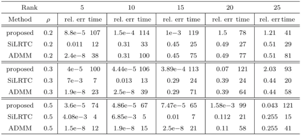
Table 1 Tensor completion results for the experiment setup from (Liu et al 2013). Values in the table are mean values of relative error and time (in seconds) over 100 random realizations. ρis the fraction of known elements in a tensor.
Rank 5 10 15 20 25
Method ρ rel. err time rel. err time rel. err time rel. err time rel. err time proposed 0.2 8.8e−5 107 1.5e−4 114 1e−3 119 1.5 78 1.21 41
SiLRTC 0.2 0.011 12 0.31 33 0.45 25 0.49 27 0.51 29 ADMM 0.2 2.4e−8 38 0.31 100 0.45 75 0.49 77 0.51 81 proposed 0.3 4e−5 100 4.44e−5 106 3.89e−4 113 0.07 121 2.03 93 SiLRTC 0.3 7e−3 7 0.013 13 0.29 24 0.39 24 0.44 20 ADMM 0.3 1.9e−8 23 2.5e−8 39 0.29 71 0.39 64 0.44 58 proposed 0.5 3.6e−5 74 4.86e−5 67 7.47e−5 65 1.58e−3 99 0.043 121
SiLRTC 0.5 4.08e−3 4 6.85e−3 5 0.01 7 0.112 21 0.255 15 ADMM 0.5 1.5e−8 12 1.9e−8 15 2.5e−8 21 0.11 58 0.255 41
of augmented Lagrangian of the problem (10)) was set to the standard deviation of the set of elements of XΩ (as suggested in (Tomioka et al. (2011)1)), error
tolerance was 0.001, and maximal number of iterations was 2000.
The results are shown in Table 1. Values in the table are mean values of relative error and time. Relative error was calculated as
ˆ X−X ΩC, F kXkΩC, F (18)
where ˆX denotes the output of the algorithm and k · kΩC, F denotes the error calculated only on the setΩC. The above defined relative error was referred to as generalization error in (Tomioka et al. (2011)1). It should be noted that the results in Table 1 differ from the results reported in (Liu et al 2013) since we couldn’t reproduce them. Also, in (Liu et al 2013) they considered onlyρ= 0.3 andρ= 0.5. It can be seen that in our simulations the proposed method outperformed the nuclear norm minimization methods from (Liu et al 2013) and (Tomioka et al. (2011)1), especially forρ= 0.2. It found the true solution in all simulations when rank was≤15. The relative error for SiLRTC was above 1e−3 in all simulations. In any case, this experiment shows that the proposed method can yield accurate solutions when the fraction of known entries, as well as the underlying tensorn -ranks are low. It also shows that the proposed method is not too sensitive to rank estimations. On the contrary, in (Gandy et al 2011) and (Tomioka et al. (2011)1) it was stated that the Tucker factorization-based method for tensor completion is too sensitive to rank estimates.
3.2 Experimental setup 2
In the second experiment, setup from (Tomioka et al. (2011)1) was used. Namely, tensor size was 50×50×20. The elements of the core tensor were generated
i.i.d. from standard normal distribution. The elements of factor matrices were also generated i.i.d. from standard normal distribution, but every factor matrix was orthogonalized (through QR factorization). Multilinear rank of the tensor was set to (7,8,9) in all simulations. For this value of multilinear rank, the method proposed in (Tomioka et al. (2011)1) generally requires at least 35 percent known tensor entries to be able to reconstruct it (see Figure 5.3 in that paper). Here we demonstrate that the method proposed here can reconstruct the underlying tensor for even lower fraction of known elements. MATLAB code for reproducing the results from (Tomioka et al. (2011)1) was taken from3and used in this experiment. The parameters of the method proposed here were as follows. Rank estimations ˆ
riwere set to 2ri, whereri denote the true ranks (7, 8 and 9). ˆXwas initialized by
randncommand in MATLAB, wherein known elements are set to their true values.
Maximal number of iterations was set to 400. Nonlinear conjugate gradient method implemented in the Poblano toolbox was used, as in the previous experiment. However, here we have also used a gradient descent with backtracking line search, initialized with the output of the nonlinear conjugate gradient method, since we found that it can increase the accuracy of the solution. We have included only the ‘constraint’ approach from (Tomioka et al. (2011)1) in the comparison for simplicity, but it can be seen from Figure 5.1 in that paper that it outperformed other approaches proposed there on this problem setting.
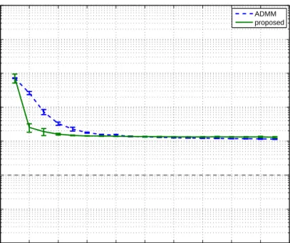
Obtained results are shown in Figure 1. It can be seen that the proposed method can reconstruct the underlying low-n-rank tensor even for small num-ber of observed entries (for 20 percent or more), smaller than the nuclear norm minimization approach, despite the fact that the ranks were significantly overes-timated. This is a clear advantage of the proposed method compared to Tucker factorization-based method used for comparison in (Tomioka et al. (2011)1).
It should be said that the proposed method does not perform well in another synthetic experiment from (Tomioka et al. (2011)1). Namely, they considered rank-(50,50,5) tensor with dimensions 50×50×20. This tensor is low-rank only in mode 3. Therefore, this problem can be treated as a matrix completion problem after matricization in mode 3. The proposed method could not compete with matrix completion approach in this experiment, especially if the true ranks were unknown.
3.3 Experimental setup 3
We also compare the proposed method with another nuclear norm minimization method from (Gandy et al 2011). We use their problem setup, which is as fol-lows. The elements of the core tensor were generated i.i.d. from standard normal distribution. In (Gandy et al 2011) it wasn’t specified how the elements of factor matrices were generated. We generated them from standard normal distribution. In the first setting, the size of the tensor was 20×20×20×20×20, all n-mode ranks were set to 2, and the fraction of known entries of the tensor was 0.2. It was demonstrated in (Gandy et al 2011) that a Tucker factorization with missing data implemented in theN-way toolbox (Andersson and Bro 2000) for MATLAB outperforms their method when exact ranks are given to the Tucker factorization algorithm. However, already if the ranks are overestimated as ˆri = ri + 1, the
0 0.1 0.2 0.3 0.4 0.5 0.6 0.7 0.8 0.9 1 10−4 10−3 10−2 10−1 100 101 102
Fraction of observed elements
Generalization error
ADMM proposed
Fig. 1 Comparison of the generalization error vs. fraction of known elements with the method from (Tomioka et al. (2011)1 ). The graph shows mean values and standard deviations of the generalization error over 50 realizations of the low-n-rank tensor and indices of the observed tensor elements.
algorithm fails to recover the underlying tensor. Here we demonstrate that the method proposed here is not too sensitive with respect to rank estimates. For the proposed method, the unknown elements in the initial approximation were set randomly, from standard normal distribution. In all experiments except the last one, rank estimates ˆrin the proposed algorithm were set to r+ 10 (ranks along every mode are equal in a single experiment, so we denote them byr). In the last experiment, we also include a result using ˆr=r+ 5, since the result obtained with ˆ
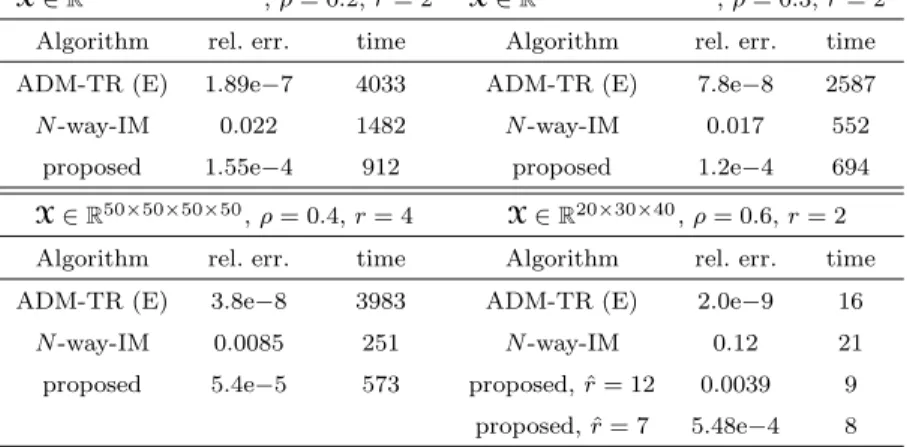
r=r+ 10 was slightly less accurate, as can be seen in Table 2. We compare our results, which are obtained as means over 20 random realizations of the tensor, with those in (Gandy et al 2011) in Table 2. We have also tested our method on other problem settings from (Gandy et al 2011). All the results are shown in Table 2. Note that the algorithm for Tucker factorization with missing data fromN-way toolbox (Andersson and Bro 2000) performed (much) worse than the proposed method, although the ranks were only slightly overestimated: ˆri =ri+ 1. On the
other hand, the proposed method yielded accurate results for ˆri=ri+ 10.
3.4 Experimental setup 4
To illustrate good performance of the proposed method, we also show some image inpainting examples. The first example is shown in Figure 2. The image of a castle, taken from the Berkeley segmentation dataset (Martin et al 2001), was artificially made low rank. This was done because natural images are generally not
low-Table 2 Tensor completion results for the experiment setup from (Gandy et al 2011). Values in the table are mean values of relative error and time (in seconds) over 20 random realizations. ρis the fraction of known elements in a tensor. ADM-TR (E) refers to alternating direction method with exact update proposd in (Gandy et al 2011).N-way IM refers to the algorithm for Tucker factorization with missing data and incorrect model information used in (Gandy et al 2011)
X∈R20×20×20×20×20, ρ= 0.2, r= 2 X∈R20×20×20×20×20, ρ= 0.3, r= 2
Algorithm rel. err. time Algorithm rel. err. time ADM-TR (E) 1.89e−7 4033 ADM-TR (E) 7.8e−8 2587
N-way-IM 0.022 1482 N-way-IM 0.017 552
proposed 1.55e−4 912 proposed 1.2e−4 694 X∈R50×50×50×50, ρ= 0.4, r= 4 X∈R20×30×40, ρ= 0.6, r= 2
Algorithm rel. err. time Algorithm rel. err. time ADM-TR (E) 3.8e−8 3983 ADM-TR (E) 2.0e−9 16
N-way-IM 0.0085 251 N-way-IM 0.12 21
proposed 5.4e−5 573 proposed, ˆr= 12 0.0039 9 proposed, ˆr= 7 5.48e−4 8
Table 3 Comparison of reconstruction quality depending on rank estimates for the image from Figure 2. Values in the table are peak signal-to-noise ratios (PSNR-s) in decibels (dB).
Rank
30 35 50 60
28.29 31.98 49.2 25.4
rank, and therefore direct rank minimization methods can not be expected to work very well in this case. When the image was not made low-rank, nuclear norm minimization method from (Liu et al 2013) performed much better than the method proposed here. However, in that case there are methods that are specialized for inpainting problems and therefore perform much better than nuclear norm minimization (for example, (Mairal et al 2008)). The ranks of the image along spatial modes were set to 40, while the parameters of the proposed methods were as follows. Rank estimates in modes 1 and 2 were set to 50. Missing pixels were initialized as the mean of observed pixels. Maximal number of iterations was set to 200. For this number of iterations, the algorithm took about 22 minutes (the algorithms from (Tomioka et al. (2011)1) took about 42 minutes for 5000 iterations).
Of course, the reconstruction quality depends on rank estimates. In Table 3 we show the results obtained with different rank estimates. It can be seen that good quality of reconstruction (better than using the nuclear norm minimization) can be obtained when the true ranks are over- or even underestimated.
(a) (b)
(c) (d)
Fig. 2 Inpainting experiments on an artificially low-rank color image. (a) Original image that was artificially made low-rank. Image size is 481×321×3. Ranks along modes 1 and 2 were set to 40. (b) Image with 80 percent pixels removed. (c) Reconstruction using the method from (Tomioka et al. (2011)1). PSNR value is 28.85 dB. (d) Reconstruction using the proposed method. Rank estimates were set to 50. PSNR value is 49.2 dB
3.5 Experimental setup 5
We also compare the proposed method with the nuclear norm minimization method from (Tomioka et al. (2011)1) on a semi-realistic amino acid fluorescence dataset (Bro 1997). This data set consists of five simple laboratory made samples mea-sured by fluorescence, with each sample containing different amounts of three amino acids. The dimensions of the original data tensor are 5×201×61. Since each individual amino acid gives a rank-one contribution to the data, the tensor is approximately rank-(3,3,3). Rank estimates in the proposed method were set to (6,6,6). Only the ‘constraint’ approach from (Tomioka et al. (2011)1) was in-cluded in the comparison, as a representative of methods considered in (Tomioka et al. (2011)1). There, it was shown that nuclear norm minimization outperformed Tucker factorization-based approach (both with correct and incorrect rank infor-mation). However, Figure 3 shows that the method proposed here performed a little better than the nuclear norm minimization method from (Tomioka et al. (2011)1). 0 0.1 0.2 0.3 0.4 0.5 0.6 0.7 0.8 0.9 1 10−4 10−3 10−2 10−1 100 101 102
Fraction of observed elements
Generalization error
ADMM proposed
Fig. 3 Generalization performance of the proposed method and the ADMM method for nu-clear norm minimization from (Tomioka et al. (2011)1)
4 Conclusions
We have proposed a Tucker factorization-based approach to low-n-rank tensor completion using similar approach as in (Acar et al 2011), where it was used for PARAFAC decomposition with missing data. The idea is to fit the Tucker model to observed tensor elements only. It was demonstrated that the proposed method can recover the underlying low-n-rank tensoreven when the true tensor ranks are unknown. This is the essence of the proposed approach. An important assumption was that the true ranks can be overestimated. However, approximate reconstruc-tion can be obtained when the ranks are underestimated. This is in contrast to Tucker-factorization algorithm with missing data from (Andersson and Bro 2000) that was used in comparative performance analysis in several recent papers on low-n-rank tensor completion. There, it was shown that the Tucker factorization-based method (Andersson and Bro 2000) is too sensitive to rank estimates. As another contribution, we show that the proposed method performs better than nuclear norm minimization methods when the fraction of known tensor elements is low.
Of course, there are no theoretical guarantees for the proposed method (since it is based on non-convex optimization), which is its main flaw. Here, we have con-centrated on numerical demonstrations only. Still, we believe that the results are interesting since they show potential advantages of non-convex methods compared to methods based on convex relaxation(s) of the rank function.
Since the proposed approach is based on unconstrained optimization, possible extensions include introducing some constraints on the factors in the model, for example orthogonality or non-negativity.
Acknowledgements This work was supported through grant 098-0982903-2558 funded by the Ministry of Science, Education and Sports of the Republic of Croatia. The authors would like to thank the project leader Ivica Kopriva. Also, the authors would like to thank the anonymous reviewer whose comments helped us to improve the manuscript.
References
Acar E, Dunlavy DM, Kolda TG, Mørup M (2011) Scalable tensor factorizations for in-complete data. Chemometrics and Intelligent Laboratory Systems 106(1):41–56, DOI 10.1016/j.chemolab.2010.08.004
Andersson CA, Bro R (1998) Improving the speed of multi-way algo-rithms:: Part i. tucker3. Chemometrics and Intelligent Laboratory Sys-tems 42(1-2):93 – 103, DOI 10.1016/S0169-7439(98)00010-0, URL http://www.sciencedirect.com/science/article/pii/S0169743998000100
Andersson CA, Bro R (2000) The n-way toolbox for matlab. Chemometrics and In-telligent Laboratory Systems 52(1):1 – 4, DOI 10.1016/S0169-7439(00)00071-X, URL http://www.sciencedirect.com/science/article/pii/S016974390000071X
Bro R (1997) Parafac. tutorial and applications. Chemometrics and Intelligent Laboratory Systems 38(2):149 – 171, DOI 10.1016/S0169-7439(97)00032-4, URL http://www.sciencedirect.com/science/article/pii/S0169743997000324
Candes EJ, Recht B (2009) Exact matrix completion via convex optimization. Founda-tions of Computational Mathematics 9:717–772, DOI 10.1007/s10208-009-9045-5, URL http://dx.doi.org/10.1007/s10208-009-9045-5
De Lathauwer L, De Moor B, Vandewalle J (2000) A multilin-ear singular value decomposition. SIAM Journal on Matrix Analy-sis and Applications 21(4):1253–1278, DOI 10.1137/S0895479896305696,
URL http://epubs.siam.org/doi/abs/10.1137/S0895479896305696, http://epubs.siam.org/doi/pdf/10.1137/S0895479896305696
Dunlavy DM, Kolda TG, Acar E (2010) Poblano v1.0: A matlab toolbox for gradient-based optimization. Tech. Rep. SAND2010-1422, Sandia National Laboratories, Albuquerque, NM and Livermore, CA
Gandy S, Recht B, Yamada I (2011) Tensor completion and low-n-rank tensor recovery via convex optimization. Inverse Problems 27, URL http://dx.doi.org/10.1088/0266-5611/27/2/025010
H˚astad J (1990) Tensor rank is np-complete. Journal of Algo-rithms 11(4):644 – 654, DOI 10.1016/0196-6774(90)90014-6, URL http://www.sciencedirect.com/science/article/pii/0196677490900146
Kolda TG, Bader BW (2009) Tensor decompositions and applications. SIAM Review 51(3):455 – 500, URLhttp://dx.doi.org/10.1137/07070111X
Liu J, Musialski P, Wonka P, Ye J (2009) Tensor completion for estimat-ing missing values in visual data. In: Proc. 2009 IEEE ICCV, URL http://dx.doi.org/10.1109/ICCV.2009.5459463
Liu J, Musialski P, Wonka P, Ye J (2013) Tensor completion for estimating miss-ing values in visual data. IEEE Trans Pattern Anal Mach Int 35(1):208-220, URL http://doi.ieeecomputersociety.org/10.1109/TPAMI.2012.39
Mairal J, Elad M, Sapiro G (2008) Sparse representation for color image restoration. IEEE Trans Image Process 17(1):53–69, DOI 10.1109/TIP.2007.911828
Martin D, Fowlkes C, Tal D, Malik J (2001) A database of human segmented natural im-ages and its application to evaluating segmentation algorithms and measuring ecological statistics. In: Proc. 8th Int’l Conf. Computer Vision, vol 2, pp 416–423
Recht B, Fazel M, Parrilo P (2010) Guaranteed minimum-rank solutions of lin-ear matrix equations via nucllin-ear norm minimization. SIAM Review 52(3):471– 501, DOI 10.1137/070697835, URLhttp://epubs.siam.org/doi/abs/10.1137/070697835, http://epubs.siam.org/doi/pdf/10.1137/070697835
Tomasi G, Bro R (2005) Parafac and missing values. Chemometrics and Intelli-gent Laboratory Systems 75(2):163 – 180, DOI 10.1016/j.chemolab.2004.07.003, URL http://www.sciencedirect.com/science/article/pii/S0169743904001741
Tucker LR (1966) Some mathematical notes on three-mode factor analysis. Psychometrika 31:279–311, DOI 10.1007/BF02289464, URLhttp://dx.doi.org/10.1007/BF02289464