Kirandeep Kour1 Sergey Dolgov2 Martin Stoll3 Peter Benner1 3
Abstract
Deploying the multi-relational tensor structure of a high dimensional feature space, more efficiently improves the performance of machine learning al-gorithms. One encounters thecurse of dimension-ality, and working with vectorized data fails to preserve the data structure. To mitigate the nonlin-ear relationship of tensor data more economically, we propose the Tensor Train way Multi-level Kernel (TT-MMK). This technique combines kernel filtering of the initial input data (Kernelized Tensor Train (KTT)), stable reparametrization of the KTT in the Canonical Polyadic (CP) format, and the Dual Structure-preserving Support Vector Machine (SVM) Kernel for revealing nonlinear relationships. We demonstrate numerically that the TT-MMK method is more reliable computa-tionally, is less sensitive to tuning parameters, and gives higher prediction accuracy in the SVM clas-sification compared to similar tensorised SVM methods.
1. Introduction
In many real world applications, resulted data are high-dimensional and stored as tensors. It is also often very expensive to generate or collect the data and we assume that we are not necessarily given a large number of test and training data. Nevertheless, it remains crucial to classify the obtained, and, in the cases considered here, tensorial data points. A prototypical example of this type are fMRI brain images (Glover,2011) that come with voxel valued rather than pixel valued images and a temporal dimension. Among the most popular methods for classifying data points are support vector machines (SVM). These are based on a margin maximization and the computation of the
corres-1
Max Planck Institute for Dynamics of Complex Technical Systems, Magdeburg, Germany. 2Department of Mathematical Sciences, University of Bath, Bath, United Kingdom. 3Faculty of Mathematics, Technische Universit¨at Chemnitz, Chemnitz, Germany. Correspondence to: Kirandeep Kour < [email protected]>.
ponding weights via an optimization framework, typically the SMO algorithm (Platt,1999). These methods often show outstanding performance, but the standard SVM model ( Cor-tes & Vapnik,1995) is designed for vector-valued rather than tensor-valued data. Although tensor objects can be reshaped into vectors, much of the information inherent in the data is lost. For example, in an fMRI image, adjacent voxels usually show a similarity in the data (He et al.,2014). As a result, the transition of vector-valued SVM to tensor-valued SVM has been proposed under the name supervised tensor learning (STL) (Tao et al.,2007;Zhou et al.,2013;Guo et al.,2012). In (Wolf et al.,2007) the authors proposed to minimize the rank of the weight parameter with the ortho-gonality constraints on the columns of the weight parameter instead of the classical maximum-margin criterion and ( Pir-siavash et al.,2009) relaxed the orthogonality constraints to further improve Wolf's method. (Hao et al.,2013) consider rank-one tensor factorization of each input tensor, while (Kotsia & Patras,2011) adopted the Tucker decomposition of the weight parameter instead of rank-one tensor decom-positions to retain more structural information. (Zeng et al.,
2017) extended this by using a Genetic Algorithm (GA) prior to the Support Tucker Machine for contraction of the input feature tensor. Along with these rank-one and Tucker representations, recently the weight tensor of STL has been approximated using a Tensor Train (TT) decomposition (Chen et al.,2018). We point out that these methods are mainly focusing on a linear representation of the data. It is well known for standard classification that a linear decision boundary is often not suitable for separation of the given data.
Naturally, the goal is to design a nonlinear transformation of the data and we refer to (Signoretto et al.,2011;2012;Zhao et al.,2013) where kernel methods have been used for tensor data. These methods have in common that their approaches are based on MLSVD/HOSVD, which rely on the flattening of the tensor data. Therefore, the resulting vector and matrix dimensions are so high that the methods are prone to over-fitting. Moreover, the intrinsic tensor structure is typically lost. Thus, other approaches are desired.
Throughout scientific computing and data science the ap-proximation of tensors based on low-rank tensor formats has received much attention over recent years (Cichocki et al.,
2016;Kolda & Bader,2009;Cichocki, 2013; Liu et al.,
2015). Particularly tailored to SVM and tensor data is the method introduced in (He et al.,2014), where the authors construct structure-preserving kernels for STL. The map-ping is defined on a rank-one tensor. The authors consider a rank-one tensor decomposition coming from the Canon-ical Polyadic/ PARAFAC (CP) format (Hitchcock,1927;
1928). This kernel is known as Dual Structure-preserving Kernel (DuSK) and we discuss its properties in more detail in Section3.6. The CP approximation results in an accur-ate and efficient scheme but the CP factorization can be numerically unstable (de Silva & Lim,2008), and choosing the best rank for CP is an NP hard problem (H˚astad,1989). Lately, kernelized tensor factorizations, specifically a ker-nelized CP (KCP) factorization, have been used in (He et al.,
2017a), which is called the Multi-way Multi-level Kernel (MMK) method. Further elaborating and understanding the approach of KCP (He et al.,2017b) provides a kernelized Tucker model, inspired from (Signoretto et al.,2013). Going further into tensor decomposition, recently, kernel approximation for TT has been introduced in (Chen et al.,
2020). We had pursued similar ideas, but the results ob-tained for the datasets we will later present were not satis-factory. Hence, we tried to come up with a better exploita-tion of the data structure, which led to the results presented in this paper.
Tensor decompositions have become an indispensable tool in many learning tasks. For example, (Novikov et al.,2016) uses the TT decomposition for both the input tensor and the corresponding weight parameter in generalized linear models of machine learning. A Kernel Principal Component Analysis (KPCA), a kernel based nonlinear feature extrac-tion technique, was proposed in (Wu & Farquhar,2007). The paper (Lebedev et al.,2014) proposes a way to speed up Convolutional Neural Networks (CNN) by applying a low-rank CP decomposition on a kernel projection tensor.
1.1. Main Novelty
As can be seen from our previous discussion, tensor methods bring great potential for dealing with high-dimensional data. Nevertheless, several gaps remain, and we address these challenges through the following contributions.
• We are expanding the use of efficient learning from rank-one decomposition to a general framework by using a TT decomposition. This is more robust, stable and computationally efficient.
• We are proposing an exact expansion of a TT to the CP format, where we add two more constraints, namely the norm equilibration and the uniqueness of Singular Value Decomposition (SVD). The norm equilibration ensures equal chances of each TT core to be important and allows using same tuning parameters for all TT
cores. The uniqueness of SVD provides a stable TT decomposition, in a sense that close tensors yield close TT cores, which is in general not true. We have ob-served that this is the most crucial part of the proposed classification model, which increases the classification accuracy of STL.
• For STL to learn effectively, we regularize the input data by means of defining a best low-rank approxim-ation via kernel projection over latent factors of the tensor input.
• We also provide a kernel approximation for the best low-rank input data by defining a nonlinear mapping into the tensor product Hilbert space. This way we extract information from the low-rank tensor factors.
In order to achieve this, we structure the paper as follows. In Section2, we set the stage introducing basic definitions and important tools. The extension to the tensor format SVM is explained in Section2.3and we also introduce the Kernel-ized Support Tensor Machine (KSTM) via the kernel trick (Sec.2.2.1). In Section3we explain the entire proposed al-gorithm. In particular, In Section3we introduce the TT-CP expansion, the norm equilibrium and discuss the uniqueness of SVD along with the proposed algorithm. Section4shows a range of numerical results for standard datasets and in comparison to a variety of competing approaches.
2. Preliminaries
2.1. Tensor decompositions2.1.1. CANONICALPOLYADIC DECOMPOSITION The Canonical Polyadic (CP) decomposition of an
Mth−order tensorX ∈ RI1×I2×...×IM is a factorization into a sum of rank-one components (Hitchcock,1927) which is given elementwise as Xi1,...,iM ∼= R X r=1 a(1)i 1,ra (2) i2,r· · ·a (M) iM,r, or shortly X∼=JA (1),A(2), · · · ,A(M)K, (1) whereA(m) = ha(m)im,ri ∈ RIm×R,m = 1, . . . , M, are called factor matrices of the CP decomposition, see Fig-ure1, andRis called the CP-rank. CP can be computed via the Alternating Least Squares (ALS) method (Nion & Lathauwer,2008), but the convergence can be slow, also it is unclear how to chooseR.
2.1.2. TENSORTRAIN DECOMPOSITION
The Tensor Train (TT) (Oseledets,2011) decomposition is the basis for our proposed algorithm. The TT approximation
I2 | {z } I1 | {z } I3 |{z } X ∼= a(1) 1 a(2)1 a(3) 1 + +· · ·+ a(1) 2 a(2)2 a(3) 2 a(1) R a(2)R a(3) R
Figure 1.CP decompositions for a 3-way tensor.
of anMth
−order tensorX∈RI1×I2×...×IM is defined as Xi1,...,iM ∼= X r0,...,rM G(1)r0,i1,r1G(2)r1,i1,r2· · ·G(M)rM−1,iM,rM, X∼=hhG(1),G(2), . . . ,G(M)ii, (2) where G(m) ∈ RRm−1×Im×Rm, m = 1, . . . , M, are 3rd-order tensors called TT-cores (see Figure 2), and
R0, . . . , RM withR0=RM = 1are calledTT-ranks.
G2 r0= 1 G1 r3= 1 G3 X I2 I1 I3 I2 I1 I3 ≈ R1 R2 I1 I2 I3 R3 R0 r1 r2 I1 I2 I3
Figure 2.TT decompositions for a 3-way tensor.
The alluring capability of the TT format is its ability to perform algebraic operations directly on TT-cores avoiding full tensors. Moreover, we can compute a quasi-optimal TT approximation of any given tensor using SVD. For more details on TT foundations we refer to (Oseledets,2011).
2.2. Support Vector Machine
In this section, we review the SVM method. For a given training dataset{(xi, yi)}Ni=1, withinput dataxi∈Rmand labelsyi∈ {−1,1}, the dual-optimization problem can be
defined as follows, max α N X i=1 αi− 1 2 N X i=1 N X j=1 αiαjyiyjhφ(xi), φ xji (3) subject to 0≤αi ≤C, M X i=1 αiyi= 0. (4)
where, the unknown functionφdefines a nonlinear decision boundary with φ: xi → φ(xi). Efficient evaluation of
hφ(xi), φ xjiis done by theKernel Trickapproximation.
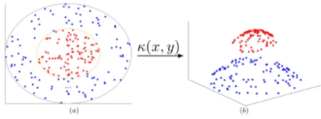
κ(x, y)
(a) (b)
Figure 3.Nonlinear mapping using kernel trick. (a) Nonlinear
classification of data inR2. (b) Linear classification in high-dimension (R3).
2.2.1. FEATUREMAP ANDKERNELTRICK
Thefeature mapis a mapφ: X → F, whereFis a Hil-bert Space (HS), the feature space. Also, every feature map is defined via a kernel such thatκi,j =κ xi,xj=
hφ(xi), φ(xj)iF. Employing properties of inner products,
[κi,j]is a symmetric positive definite matrix. This approach
is known as the kernel trick, it is used in order to get a linear learning algorithm to learn a nonlinear boundary, without explicitly knowing the nonlinear functionφ. In case of SVM, the only task needed is to choose a legitimate kernel function. That is how we work with the multi-way input data in the high-dimensional space while doing all the computation in the original low dimensional space. Figure
3illustrates the linear separation in a higher dimensional space.
2.3. Kernelized Support Tensor Machine
In our case, we have a dataset{(Xi, yi)}Ni=1with input data
in the form of a tensorXi ∈ RI1×I2×...×IM. Hence, the tensor extension of the dual nonlinear SVM from (3) can written as follows: max α N X i=1 αi−1 2 N X i=1 N X j=1 αiαjyiyjhφ(Xi), φ(Xj)i subject to 0≤αi≤C, N X i=1 αiyi= 0. (5)
The classification setup given in (5) is known as Support Tensor Machine (STM) (Tao et al.,2007). Also, the nonlin-ear feature mappingφ:X→φ(X)takes tensor input data to a higher dimensional space, similar to the vector case. Therefore, by using the kernel trick, explained in Section
2.2.1, STM can defined as follows: max α N X i=1 αi− 1 2 N X i=1 N X j=1 αiαjyiyjκ(Xi,Xj) (6) subject to 0≤αi≤C, M X i=1 αiyi = 0. (7)
We call this setup, the Kernelized STM (KSTM). For the learning algorithm KSTM, the essential term is the kernel
κ(Xi,Xj). Therefore this is the preeminent part for
com-putational aspects. We are proposing a comcom-putationally efficient kernelκ, containing all the dominant features re-quired for training and testing of the algorithm next.
2.4. Tensor Product Reproducing Kernel Hilbert Space AssumeHm,h·,·im, κ(m)
is a Reproducing Kernel Hil-bert Space (RKHS) of a functionκ(m)defined on the set
Xm, whereκ(m): Xm×Xm → Ris a reproducing ker-nel (Berlinet & Thomas-Agnan,2004) of HSHm, for any
m= 1, . . . , M, andh·,·imdefines an inner product on the
same space. Following the definition provided in ( Signor-etto et al.,2013), the spaceH=H1⊗ H2⊗ · · · ⊗ HM is
called a Tensor product RKHS (TP-RKHS) and is denoted by H,h·,·i,κwithκas areproducing kernel.
We are interested in representing functionsf(x) ∈Hof the tuplex = x(1), x(2), . . . , x(M) ∈ X, where X :=
X1×X2×· · ·×XM. This allows us to express anyf ∈H,
and hence to form the tensor product space using linear combination of tensor product (“rank-one”) functions:
f(x) =X
j
αjfj(1)1 (x1)⊗ · · · ⊗f
(M) jM (xM),
wherej= (j1, . . . , jM)is a tuple index, andfj(m)m ∈ Hm,
m= 1, . . . , M. Additionally, from the definition of RKHS on each setXmit holds that
f(x) =X j αj M Y m=1 D fj(m)m , κ (m) xm E m, (8) whereκ(m)xm =κ (m)(x
m,·)is the reproducing kernel
eval-uated at the target pointxm. This gives the tensor product
reproducing kernel
κ=κ(1)⊗ · · · ⊗κ(M).
The concept of RKHS can be used to associate a given tensor input data to a function, which allows us to filter irrelevant components from the tensor, such as the measurement noise. This is explained in Section3.5.
3. The proposed algorithm
In this paper, the whole research idea evolves around solving the basic classification problem. Further, we have given a training dataset{Xi ∈ RI1×I2×...×IM, yi}Ni=1 ⊂ X×Y,
whereXis an input tensor space andYis a set of class labels containing{−1,1}. The main accomplishment is to find a functionf:X→Y, which can approximate and predict the corresponding class labels for any test input data, while maintaining the Bias-Variance trade-off (Hastie et al.,
2001) of the predicted model.
3.1. TT-CP Expansion
Despite the numerical difficulties outlined in the introduc-tion, the simplicity of the CP decomposition makes it a convenient and intuitive tool for structuring and analyzing the input tensor data. The TT decomposition is easy to com-pute, but different TT blocks might have different scales; besides, they may be not unique. This complicates the TT data classification with SVM. In this section, we propose a combined representation to elucidate both of these obstacles. First, we compute a TT decomposition of the data in order to get a robust approximation. Second, the resulting TT-cores are converted into the CP format keeping the structure of the original data. This means the data is basically coming from TT cores, while being structured in CP format. This can be done in the following manner.
Let the TT approximation of the inputX∈RI1×I2×I3be Xi1,i2,i3 = X r1,r2 G(1)i 1,r1G (2) r1,i2,r2G (3) r2,i3
then we can merger1, r2into one indexr=r1+(r2−1)R1
and write a CP decomposition,
Xi1,i2,i3 =
RX1R2
r=1
Hi(1)1,rHi(2)2,rHi(3)3,r,
where the CP factors are defined as
Hi(1)1,r =G (1) i1,r11r2, Hi(2)2,r =G(2)r1,i2,r2, Hi(3)3,r =1r1G (3) r2,i3,
using1for a vector of all ones. This is simply rearranging of the data using permutation and reshaping from one form of a tensor decomposition to another (TT to CP). Notice that this expansion is exact and actually does not need any new computations (only copying of data). In particular, the CP factors can be computed in Matlab using the following commands: H1 = reshape(permute(G1,[2,1,3]),I1,R1); H1 = kron(ones(1,R2), H1); H2 = reshape(permute(G2,[2,1,3]),I2,R1*R2); H3 = reshape(permute(G3,[2,1,3]),I3,R2); H3 = kron(H3, ones(1,R1));
3.2. Norm Equilibration
The above explained TT-CP expansion is used in our pre-liminary version of the kernel for solving the optimization problem (6). However, this did not lead to better classi-fication results. Notice that (He et al., 2017a) used the CP-ALS algorithm (Nion & Lathauwer,2008) to compute a CP decomposition, in which the norms of all CP vectors
a(1)r , . . . ,a(M)r for the samerwere equal. In contrast, the
plain TT-SVD algorithm (Oseledets,2011) does not enforce the norm equilibration itself. Therefore, we add the norm equilibrium constraint to the TT-CP expansion. We have found it to be one key ingredient for the successful applica-tion of the proposed TT-SVM method.
For each given input tensorX ∈ RI1×I2×I3, the TT-CP
expansion isJH(1), H(2), H(3)
Kwith rankr, where we use
the so-called Kruskal notation from (1). The norm equilib-ration of the first core of the TT-CP expansion is completed in the following way,
kNrk= Hr(1) ∗Hr(2) ∗Hr(3) , Hr(1):= Hr(1) Hr(1) ∗k Nrk1/3, Hr(1):=Hr(1)∗ Hr(2) ∗Hr(3) 1/3 Hr(1) 2/3 .
A similar approach has been used for each core of each input tensor. The motivation behind norm equilibrium is to distribute equal chances to each core to be important enough in terms of accumulating the original data in it.
3.3. Uniqueness of SVD
Since the TT decomposition is computed using the SVD (Oseledets, 2011), the particular factors G(1),G(2),G(3)are defined only up to a sign indeterminacy. For example, in the first step we compute the SVD of the 1-mode unfolding,
X(1)=σ1u1v1>+· · ·+σI1uI1v
>
I1,
followed by truncating the expansion at rankR1or
accord-ing to the accuracy threshold ε, choosing R1 such that
σR1+1 < ε. However, any set of vectors{ur1, vr1} can
be replaced by{−ur1,−vr1}without changing the whole
tensor. While this is not an issue for data compression, clas-sification using TT factors can be affected significantly by this indeterminacy. For example, tensors that are close to each other should likely produce the same label. In contrast, even a small difference in the original data may lead to a different sign of the singular vectors, and the SVM might assign different labels to such factors.
To circumvent this issue, we fix the signs of the singular vectors as follows. For eachr1 = 1, . . . , R1, we find the
position of the maximum in modulus element in the left sin-gular vector,i∗= arg maxi|ur1(i)|, and make this element
positive, ¯
ur1 :=ur1/sign(ur1(i∗)), v¯r1 :=vr1·sign(ur1(i∗)).
Finally, we collectu¯r1into the first TT core,G
(1)(i 1, r1) =
¯
ur1(i1), and continue with the TT-SVD algorithm using¯vr1
as the right singular vectors. In contrast to the sign, the whole dominant singular termsur1v
>
r1 depend continuously
on the input data, and so do the maximum absolute elements. This ensures that close tensors produce close TT cores.
3.4. Noisy Data and Threshold
Generally, data coming from real world applications are affected by measurement or preprocessing noise. This can affect both computational and modeling aspects, increasing the TT ranks (since a tensor of noise lacks any meaningful TT decomposition), and spoiling the classification if the noise is too large. However, SVD can serve as a de-noising algorithm automatically: the dominant singular vectors are often “smooth” and hence represent a useful image, while the latter singular vectors are more oscillating and capture primarily the noise. Therefore, it is actually beneficial to compute the TT approximation with deliberately low TT ranks / large truncation threshold. On the other hand, the TT rank must not be too low in order to approximate the features of the tensor with sufficient accuracy. Since the precise magnitude of the noise is unknown, we carry out a cross-validation test to find the optimal TT rank.
3.5. Kernelized Tensor Train (KTT)
Tensor decompositions can provide a compact form, while containing the multi-way array structure and keeping the meaning of tensor input data. However, we may need to regularize the underlying input tensor data, so that inform-ation can be captured well enough by the learning model (STL). This regularization for the learning model has been proposed for rank-one decomposition of data in (Signoretto et al.,2013), and is based on RKHS.
Therefore, for getting most out of all the latent struc-tural features of a tensor, we treat anM-th order tensor X∈RI1×I2×...×IMas an element of the TP-RKHSH, and assume that it has low-rank structure in spaceH, such that the following fitting criterion holds (He et al.,2017b):
f?=argmin fjm(m) X i Xi− X j M Y m=1 D fj(m)m , κ(m)xim E m 2 (9) =⇒ min F(m) X−JK(1)F(1),· · · , K(M)F(M)K 2 F, (10)
whereK(m)
∈ RIm×Im andF(m) ∈ RIm×Jm consist of samples ofκ(m)andf(m)
jm , respectively. This formulation is called Kernelized Tensor Factorization (KTF).
In particular, we are using the TT-CP expansion as a tensor factorization for KTF and we call it Kernelized Tensor Train (KTT). The formulation of a kernelized projection on tensor input dataXwas demonstrated in (Lebedev et al.,2014) for the CP-decomposition, which achieves considerable spee-dups with minimal loss in accuracy. Acknowledging it and using (Bazerque et al.,2012), we extend the rank-one idea to TT-CP and work towards getting a best KTT approximation. For keeping it simple, without loss of generality, let the input is a 3-dimensional tensorX∈RI×J×K, with the TT-CP expansionJH(1), H(2), H(3)
K. In order to get the the
kernel version of the tensor factorization cores, we define a mapping from input tensor to TT-CP expansion cores. Fol-lowing the (Bazerque et al.,2012), a nonparametric function
f:X×Y×Z→Ris introduced such that
FR= f:f(x, y, z)7→ R X r=1 ˆ h(1)r (x)ˆh(2)r (y)ˆh(3)r (z), s.t. ˆh(1)r ∈ H1,ˆh(2)r ∈ H2,ˆh(3)r ∈ H3 ,
whereH1,H2andH3are HS constructed with respect to
kernelsκ(1), κ(2), κ(3), respectively. From the definition of
RKHS, ˆ h(1)r (x) =PIi=1h (1) i,rκ(1)(xi, x), ˆ h(2)r (y) =PJj=1h(2)j,rκ(2) yj, y, ˆ h(3)r (z) =PKk=1h (3) k,rκ(3)(zk, z),
therefore, the interpolation of TT-CP expansion into a con-tinuous function is,
F?= ˆf(x, y, z) = R X r=1 ˆ h(1)r (x)ˆh(2)r (y)ˆh(3)r (z).
Hence, the optimization problem mentioned in (9) can be written in the following parametric way (He et al.,2017a):
f?=argmin f∈FR I X i=1 J X j=1 K X k=1 xi,j,k−f xˆ i, yj, zk 2 (11) =⇒ min H(m) X−JK(1)H(1), K(2)H(2), K(3)H(3)K 2 F, (12) with kernel matrices
K(1) =hκ(1)(xi, xj) i ∈RI×I, K(2) =hκ(2)(yi, yj) i ∈RJ×J, and K(3) =hκ(3)(zi, zj) i ∈RK×K.
These kernel matrices work as a filter over latent structure along each dimension (mode) of a tensor factorization. Con-sequently, this helps to reveal the pattern of an input image data, similarly to an affine transformation of the first layer of a CNN. To simplify the presentation, we will assume that KTT form of two tensorsX,Y∈RI×J×Kdenoted by using the same notationJH(1), H(2), H(3)
K,JP
(1), P(2), P(3) K.
3.6. Nonlinear Mapping
The optimal features or the best low-rank approximation of the input tensor object have been obtained via the KTT. After this, the next step is to get the nonlinear classification boundary using KSTM. This leads to the formulation of the most expensive and prominent term in (6). Therefore, the corresponding kernel approximation will be explained further in this section.
In order to get a nonlinear classification boundary for the input tensor data. The downstream computation is that the extracted optimal features (KTT) should reach to the learning model (KSTM) efficiently. As we have seen, the KTT factorization provides factor matrices. Each of these matrices is associated with each of the tensor modes. These factor matrices can be defined in a tensor fashion by using the outer product. Therefore, we extend the idea of the MMK (He et al.,2017a) method for KTT. Hence, a nonlinear mapping from the original feature space for the KTT factors to a third-order HS can be defined in the following way Ψ :X×Y×Z7→RH1×H2×H3 Ψ : R X r=1 h(1)r ⊗h(2)r ⊗h(3)r 7→ R X r=1 φ(h(1)r )⊗φ(h(2)r )⊗φ(h(3)r ). (13) Similarly to the standard SVM, applying the kernel trick in equation (13) gives us a practically computable kernel inspired by DuSK (He et al.,2014;2017a):
hΨ(X),Ψ(Y)i ≈κ(X,Y) ≈κPRr=1h(1)r ⊗h(2)r ⊗hr(3),PRr=1p(1)r ⊗p(2)r ⊗p(3)r , =hΨ( R X r=1 h(1)r ⊗h(2)r ⊗h(3)r ),Ψ( R X r=1 p(1)r ⊗p(2)r ⊗p(3)r )i 7→ R X i,j=1 hφ(h(1)i ),φ(p(1)j )ihφ(h(2)i ),φ(p(2)j )ihφ(h(3)i ),φ(p(3)j )i ≈ R X i,j=1 κ(h(1)i , p (1) j )κ(h (2) i , p (2) j )κ(h (3) i , p (3) j ). =⇒ κ(X,Y)≈ R X i,j=1 3 Y k=1 exp − h(k)i −p(k)j 2 2σ2 . (14)
Algorithm 1Kernel approximation as an input of STM Input:dataX∈RI×J×K, rankR
1=R2=R.
Output:G(1),G(2),G(3)
(Optional) Set kernel matricesK(1), K(2), K(3).
fori, j= 1toNdo ComputehhG(1),G(2),G(3)ii ∼=Xi(TT-SVD) ComputehhU(1),U(2),U(3)ii ∼=Xj(TT-SVD) JH (1), H(2), H(3) K=hhG (1),G(2),G(3) ii(TT-CP) JP (1), P(2), P(3) K=hhU (1),U(2),U(3) ii(TT-CP) fork= 1,2,3do (Optional)H(k) ←(K(k))TH(k), KTT filtering (Optional)P(k) ←(K(k))TP(k), KTT filtering end for κ Xi,Xj≈ PR i,j=1κ h(1)i , p (1) j κh(2)i , p (2) j κh(3)i , p (3) j . end for
This kernel approximation (14) performs on each pair of tensor input data. This means on each pair of the best low-rank structure (KTT). The width parameterσ >0needs to be chosen judiciously to ensure accurate learning.
As an input of the KSTM learning model, we are using the TT-CP factors. Therefore, we call this proposed model the Tensor Train Multi-way Multi-level Kernel (TT-MMK). It fulfills the objectives of extracting optimal low-rank features, and of building a more accurate and efficient classification model. Plugging the kernel values (14) into the SVM optim-izer (6) completes the algorithm. The performance of this model is shown by numerical experiments in the next sec-tion. Along with this, the overall idea is summarized in Al-gorithm1, where the computation ofH(k)
←(K(k))TH(k)
is optional and can be switched on and off, depending on the input dataset.
4. Numerical Tests
4.1. Experimental SettingsAll the experimental implementation has been done in
MATLAB 2016b. In the first step, we compute the TT format of an input tensor using theTT-Toolbox1, where we modified the function@tt_tensor/round.mto en-force the uniqueness of SVD (Sec. 3.3). Moreover, we have implemented the TT-CP conversion, together with the norm equilibration. For the training of the TT-MMK model, we have used the svmtrainfunction available in theLIBSVM2 library. The kernel filtering matrices are chosen fromrandom, identityorcovariancematrices by
1https://github.com/oseledets/TT-Toolbox
2
https://www.csie.ntu.edu.tw/˜cjlin/ libsvm/
comparing the cross-validation errors and choosing the mat-rix providing the best accuracy. We have run all experiments on a machine equipped with Ubuntu release 16.04.6 LTS (Xenial Xerus) 64-bit, 7.7 GiB of memory, and an Intel Core i5-6600 CPU @ 3.30GHz×4 CPU.
Figure 4.3D tensor corresponding to the fMRI brain image.
4.1.1. PARAMETERTUNING
The ensemble designed model has three various parameters. First, to simplify tuning of the model to noise, we take all TT ranks equal to the same value R ∈ {1,2, . . .10}. Another parameter is the width of the Gaussian Kernelσ. Finally, the third parameter is trade-offC for the KSTM optimization technique (7). BothσandCare chosen from
{2−8,2−7, . . . ,27,28
}. For tuningR, σandCto the best classification accuracy we use thek-fold cross validation. More specifically, we use five fold cross-validation. Along with this, we run all computations 50 times and average the accuracy over these runs. This ensures confident and reproducible comparison of different techniques.
4.2. Data Collection
Alzheimer Disease (ADNI): The ADNI stands for Alzheimer Disease Neuroimaging Initiative. This dataset is collected from ADNI3. It contains the resting state fMRI images of 33 subjects. The dataset was collected from the authors of the paper (He et al.,2017a). The data contain two labels, one stands for Mild Cognitive Impairment (MCI) or Alzheimer Disease (AD), and normal controls. The sample size is61×73×61 = 271633. The AD+MCI is labeled with−1, and the normal control is labeled with1. Prepro-cessing of datasets is explained in (He et al.,2014). Attention Deficit Hyperactivity Disorder (ADHD):The ADHD dataset is collected from ADHD-200 global compet-ition dataset4. It is a publicly available preprocessed fMRI
dataset from eight different institutes, collected at one place. The dataset is unbalanced, so we have chosen 200 subjects randomly. The classification labels are ADHD patient (−1)
3http://adni.loni.usc.edu/
4http://neurobureau.projects.nitrc.org/
and healthy person (1). Each of the 200 resting state fMRI samples contains49×58×47 = 133574voxels.
4.3. Methods Compared
We compare the classification accuracy of the proposed TT-MMK method with the accuracy of the following existing approaches.
SVM:This is the standard SVM with Gaussian Kernel. This is the most used optimization method for vector input based on maximum margin technique.
STuM: The Support Tucker Machine (STuM) (Kotsia & Patras,2011) uses the Tucker decomposition. The weight parameters of SVM are computed for optimization into Tucker factorization form.
DuSK: The idea of DuSK (He et al.,2014) is based on defining the kernel approximation for the rank-one decom-position. This is one of the first methods in this direction. MMK:This method is an extension of DuSK to the KCP input. It uses the covariance/random matrix projection over the CP factor matrices, to get a KCP for the given input tensor (He et al.,2017a).
Improved MMK:This is a slightly improved MMK, where identity matrices are used for projecting CP onto KCP in-stead of the covariance/random matrices. This we found out and named it as Improved MMK.
TT-MMK:This is Algorithm1proposed in this paper.
4.4. Results
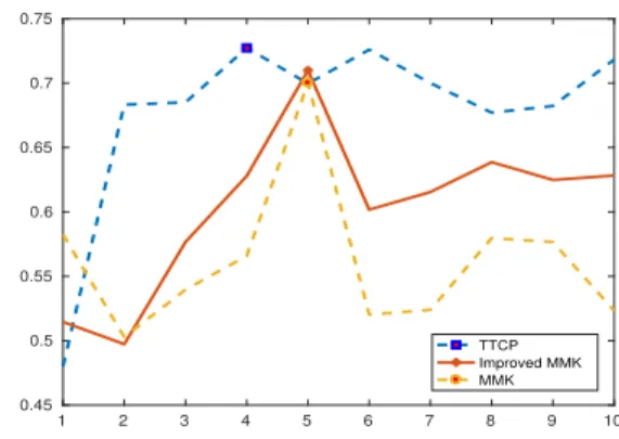
We used original codes provided by the authors of the paper (He et al.,2017a) for comparing the DuSK and MMK meth-ods to our methmeth-ods. Our key observations are as follows. (In)sensitivity to the TT rank selection: Figure5, show that the proposed method gives almost the same accuracy for different TT ranks. For some samples, even the TT rank 2gives good classification. Note that this is not the case for MMK, which requires a careful selection of the CP rank. Kernel filtering: the best accuracy is achieved with the identity filter. This may indicate that the TT decomposition captures already a resolution that is just about right, such that no further filtering is needed. We anticipate that pre-filtering might be necessary for larger noise levels, though. Computational robustness:while the CP decomposition can be computed using only iterative methods in general, all steps of the kernel computation in TT-MMK are “direct” in a sense that they require a fixed number of established linear algebra operations, such as SVD and matrix products. Classification accuracy: the proposed method gives the best average classification accuracy (over73%), compared to five other state of the art techniques.
In addition to the TT-MMK method as described in Al-gorithm1, we tried also a straightforward implementation
Table 1.Average classification accuracy for different methods and
datasets
METHODS ADNI ADHD
SVM 49 % 52% STUM 51 % 54% DUSK 55 % 58% MMK 69 % 60% IMPROVEDMMK 71 % 61% TT-MMK 73% 64%
of the DuSK Kernel (14) for the TT cores obtained directly from the TT-SVD approximation, without enforcing the uniqueness of SVD, the TT-CP conversion and the norm equilibration. A similar approach was recently proposed in (Chen et al.,2020). However, for the ADNI dataset this “simplified” TT-MMK gives only an accuracy of 60%, which is lower than the accuracy of the MMK (He et al.,2017a) method. This demonstrates that all steps of the unification procedure proposed in Section3are important for a reliable TT-SVM classification. 1 2 3 4 5 6 7 8 9 10 0.45 0.5 0.55 0.6 0.65 0.7 0.75 TTCP Improved MMK MMK
Figure 5.Accuracy of TT-MMK (TTCP), MMK and Improved
MMK methods for the ADNI dataset using different TT/CP ranks respectively. TT-MMK and Improved MMK methods use identity kernel filtering while the MMK uses random kernel filtering.
5. Conclusion
We have proposed a new kernel model for SVM classific-ation of tensor input data. Our kernel extends the DuSK approach (He et al.,2017a) to the TT decomposition of the input tensor with enforced uniqueness. The TT de-composition can be computed more reliably than the CP decomposition used in the original DuSK kernel. Using classical fMRI benchmark datasets, we have demonstrated that the new TT-DuSK method provides higher classifica-tion accuracy for an unsophisticated choice of the TT ranks. We have also found out that the uniqueness constraints are
crucial for achieving this accuracy. Further research will consider improving the computational complexity of the current scheme, as well as a joint optimization of TT cores and SVM weights. Similarly to the neural network compres-sion in the TT format (Novikov et al.,2015), such a targeted iterative refinement of the TT decomposition may improve the prediction accuracy.
Acknowledgment
This work is supported by the International Max Planck Research School for Advanced Methods in Process and System Engineering-IMPRS ProEng, Magdeburg. The authors are grateful to Lifang He for providing codes for the purpose of comparison.
References
Bazerque, J. A., Mateos, G., and Giannakis, G. B. Nonpara-metric low-rank tensor imputation. InIEEE Statistical Signal Processing Workshop (SSP), pp. 876–879, 2012. Berlinet, A. and Thomas-Agnan, C. Reproducing Kernel
Hilbert Space in Probability and Statistics. 01 2004. Chen, C., Batselier, K., Ko, C.-Y., and Wong, N. A support
tensor train machine.arXiv preprint arXiv: 1804.06114, 2018.
Chen, C., Batselier, K., Yu, W., and Wong, N. Ker-nelized support tensor train machines. arXiv preprint arXiv:2001.00360, 2020.
Cichocki, A. Tensor decompositions: A new concept in brain data analysis. arXiv preprint arXiv:1305.0395, 2013.
Cichocki, A., Lee, N., Oseledets, I., Phan, A.-H., Zhao, Q., and Mandic, D. P. Tensor networks for dimensionality reduction and large-scale optimization: Part 1 low-rank tensor decompositions.FNT in Machine Learning, 9(4-5): 249–429, 2016.
Cortes, C. and Vapnik, V. Support-vector networks. Ma-chine Learning, 20:273–297, 1995.
de Silva, V. and Lim, L.-H. Tensor rank and the ill-posedness of the best low-rank approximation problem. SIAM J. Matrix Anal. Appl., 30(3):1084–1127, 2008. Glover, G. H. Overview of functional magnetic resonance
imaging.Neurosurgery Clinics of North America, 22(2): 133 – 139, 2011.
Guo, W., Kotsia, I., and Patras, I. Tensor learning for re-gression. IEEE Transactions on Image Processing, 21(2): 816–827, 2012.
Hao, Z., He, L., Chen, B., and Yang, X. A linear sup-port higher-order tensor machine for classification.IEEE Transactions on Image Processing, 22(7):2911–2920, 2013.
H˚astad, J. Tensor rank is np-complete. InAutomata, Lan-guages and Programming, pp. 451–460, Berlin, Heidel-berg, 1989. Springer Berlin Heidelberg.
Hastie, T., Tibshirani, R., and Friedman, J. The Elements of Statistical Learning. Springer Series in Statistics. Springer New York Inc., New York, USA, 2001. He, L., Kong, X., Yu, P. S., Ragin, A. B., Hao, Z., and Yang,
X. Dusk: A dual structure-preserving kernel for super-vised tensor learning with applications to neuroimages. CoRR, abs/1407.8289, 2014.
He, L., Lu, C.-T., Ding, H., Wang, S., Shen, L., Yu, P. S., and Ragin, A. B. Multi-way multi-level kernel modeling for neuroimaging classification. InThe IEEE Conference on Computer Vision and Pattern Recognition (CVPR), pp. 6846–6854, 2017a.
He, L., Lu, C.-T., Ma, G., Wang, S., Shen, L., Yu, P. S., and Ragin, A. B. Kernelized support tensor machines. InProceedings of the 34th International Conference on Machine Learning-Volume 70, pp. 1442–1451, 2017b. Hitchcock, F. L. The expression of a tensor or a polyadic as
a sum of products.Journal of Mathematics and Physics, 6(1-4):164–189, 1927.
Hitchcock, F. L. Multiple invariants and generalized rank of a p-way matrix or tensor. Journal of Mathematics and Physics, 7(1-4):39–79, 1928.
Kolda, T. G. and Bader, B. W. Tensor decompositions and applications.SIAM Review, 51(3):455–500, 2009. Kotsia, I. and Patras, I. Support tucker machines. CVPR
2011, pp. 633–640, June 2011.
Lebedev, V., Ganin, Y., Rakhuba, M., Oseledets, I. V., and Lempitsky, V. S. Speeding-up convolutional neural networks using fine-tuned CP-decomposition. CoRR, abs/1412.6553, 2014.
Liu, X., Guo, T., He, L., and Yang, X. A low-rank approximation-based transductive support tensor machine for semisupervised classification.IEEE Transactions on Image Processing, 24(6):1825–1838, 2015.
Nion, D. and Lathauwer, L. D. Fast communication: An enhanced line search scheme for complex-valued tensor decompositions. Application in DS-CDMA. Signal Pro-cessing, 88(3):749–755, 2008.
Novikov, A., Podoprikhin, D., Osokin, A., and Vetrov, D. P. Tensorizing neural networks. InAdvances NIPS 28, pp. 442–450. 2015.
Novikov, A., Trofimov, M., and Oseledets, I. V. Exponential machines. arXiv preprint arXiv:1605.03795, 2016. Oseledets, I. V. Tensor-train decomposition. SIAM Journal
on Scientific Computing, 33(5):2295–2317, 2011. Pirsiavash, H., Ramanan, D., and Fowlkes, C. C. Bilinear
classifiers for visual recognition. InAdvances in Neural Information Processing Systems 22, pp. 1482–1490. Cur-ran Associates, Inc., 2009.
Platt, J. C.Fast Training of Support Vector Machines Using Sequential Minimal Optimization, pp. 185–208. MIT Press, 1999.
Signoretto, M., Olivetti, E., Lathauwer, L. D., and Suykens, J. A. K. A kernel-based framework to tensorial data ana-lysis.Neural Networks, 24(8):861 – 874, 2011. Artificial Neural Networks: Selected Papers from ICANN 2010. Signoretto, M., Olivetti, E., Lathauwer, L. D., and Suykens,
J. A. K. Classification of multichannel signals with cumulant-based kernels. IEEE Transactions on Signal Processing, 60(5):2304–2314, 2012.
Signoretto, M., Lathauwer, L. D., and Suykens, J. A. Learn-ing tensors in reproducLearn-ing kernel Hilbert spaces with mul-tilinear spectral penalties. ArXiv, abs/1310.4977, 2013. Tao, D., Li, X., Hu, W., Stephen, M., and Wu, X. Supervised
tensor learning.Knowledge and Information Systems, pp. 1–42, 2007.
Wolf, L., Jhuang, H., and Hazan, T. Modeling appearances with low-rank SVM. InIEEE Conference on Computer Vision and Pattern Recognition, 2007.
Wu, M. and Farquhar, J. A subspace kernel for nonlinear feature extraction.Proceedings of the 20th International Joint Conference on Artificial Intelligence (IJCAI-07), 1125-1130 (2007), 2007.
Zeng, D., Wang, S., Shen, Y., and Shi, C. A GA-based feature selection and parameter optimization for support tucker machine. Procedia Computer Science, 111:17 – 23, 2017. The 8th International Conference on Advances in Information Technology.
Zhao, Q., Zhou, G., Adali, T., Zhang, L., and Cichocki, A. Kernelization of tensor-based models for multiway data analysis: Processing of multidimensional structured data. IEEE Signal Processing Magazine, 30(4):137–148, 2013.
Zhou, H., Li, L., and Zhu, H. Tensor regression with applica-tions in neuroimaging data analysis. Journal of the Amer-ican Statistical Association, 108(502):540–552, 2013. PMID: 24791032.