Design of multi-parametric NCO tracking controllers for linear dynamic systems
Muxin Suna, Benoˆıt Chachuata,∗, Efstratios N. Pistikopoulosb
aCentre for Process Systems Engineering, Department of Chemical Engineering, Imperial College London, London, SW7 2AZ, UK bMcFerrin Department of Chemical Engineering, Texas A&M University, College Station, TX 77843, USA
Abstract
A methodology for combining multi-parametric programming and NCO tracking is presented in the case of linear dynamic systems. The resulting parametric controllers consist of (potentially nonlinear) feedback laws for tracking optimality conditions by exploiting the underlying optimal control switching structure. Compared to the classical multi-parametric MPC controller, this approach leads to a reduction in the num-ber of critical regions. It calls for the solution of more difficult parametric optimization problem with linear differential equations embedded, whose critical regions are potentially nonconvex. Examples of con-strained linear quadratic optimal control problems with parametric uncertainty are presented to illustrate the approach.
Keywords: multi-parametric programming, NCO-tracking, feedback control, explicit MPC
1. Introduction
Driven by the need to improve performance and reduce economic costs in industrial processes, on-line optimization and real-time control have been receiving a lot of attention. Many such industrial applications involve fast dynamic systems operated under constraints, typically reflecting physical operation bounds and/or safety requirements [1]. Optimal control strategies can be determined by solving constrained op-timization problems based on a dynamic model of the system. One major challenge with this approach is how to effectively deal with uncertainty stemming from model mismatch and process disturbances, as optimal operation needs to be decided on-line using real-time feedback. The strategy employed in classical model predictive control (MPC) [2] handles this uncertainty by repeatedly solving the optimization problem on-line in order to update the optimal inputs. This is often a rather computationally demanding task that may cause serious delays especially for systems with fast dynamics, leading to suboptimal performance or even infeasibility.
Several approaches have been proposed in the literature to overcome the need for repeatedly solving optimization problems on-line. In the multi-parametric programming paradigm [3], the optimization is performed off-line, resulting in a priori explicit mapping of the solutions, effectively control strategies, as a function of measurable quantities. For continuous-time systems, this approach calls for the solution of multi-parametric dynamic optimization problems (mp-DO) [4].
In practice, such mp-DO can either be transformed into a finite-dimensional multi-parametric program via control vector parameterization [4] or handled directly into its native infinite-dimensional form using
∗
Corresponding author.
Email addresses:[email protected](Muxin Sun),[email protected](Benoˆıt Chachuat),
[email protected](Efstratios N. Pistikopoulos)
the corresponding optimality conditions. In the context of solving the finite-dimensional multi-parametric program, there exist numerous publications [3,5–10], whereas solving the infinite-dimensional counterpart has received relatively little attention [4].
Parametric optimal solutions for the latter can be obtained by sensitivity analysis, also known as neigh-boring extremal (NE) control. In this approach a feedback law is derived in the neighborhood of a nominal solution, where the switching structure—namely, the sequence of active path and terminal constraints— remains the same [11–14]; see also [12, 15, 16] for a discussion of the differentiability and stability of parametric solutions. For constrained linear-quadratic optimal control problems in particular, Sakizlis and coauthors [4] have shown that the mp-DO can be written as a multi-parametric boundary value problem using the Pontryagin Minimum Principle [17–19]. The continuous-time optimal control trajectory is ex-pressed as a time-varying functions of selected parameters, which provides a means for determining the control switching structure using standard multi-parametric programming techniques.
Another approach to reducing the on-line computational burden involves tracking the necessary condi-tions for optimality, namely NCO-tracking [20,21]. There, an optimal control policy is obtained indirectly by forcing the NCOs to zero. Such a forcing requires knowledge of the switching structure of the optimal control, based on which feedback control laws can be derived on account of the available output measure-ments, effectively converting an optimal control problem into a set of self-optimizing feedback control laws [20,22]. However, a key assumption for this controller to enable optimal or even feasible operation is that the switching structure should remain unchanged, which may not be the case when large uncertainty is present.
This paper presents a methodology for combining mp-DO and NCO-tracking into a unified framework for model predictive control, for which we coin the namemulti-parametric NCO-tracking control. Such a combination is especially promising in that multi-parametric programming provides a means for relaxing the fixed switching structure assumption in NCO-tracking, thereby paving the way towards a theoretical justification for NCO-tracking too. In addition, the use of feedback laws tracking the optimality conditions inside multi-parametric controller provides a means for reducing the number of critical regions compared with classical mp-MPC controllers based on control vector parameterization.
The rest of the paper is organized as follows. Sect. 2 provides some background for both multi-parametric programming and NCO tracking method. Sect.3presents the multi-parametric NCO-tracking methodology, including the use of mp-DO for mapping subregions of the uncertain parameters to various switching structure and the implementation of the corresponding NCO-tracking controllers in a receding horizon manner. Several numerical examples are given in Sect.4to illustrate the approach. Finally, Sect.5
concludes the paper.
2. Background
2.1. Multi-parametric MPC
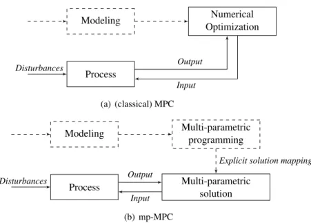
Multi-parametric programming provides a means for computing the solution mapping of an optimization-based control problem off-line, based on a model of the dynamic system. The optimal con-trol trajectory is expressed as a function of given parameters, usually some uncertain measured quantities, thus avoiding the need for repeatedly solving optimization problems on-line when these parameters vary [5,6,9,23,24]. In the context of MPC, this approach is referred to as mp-MPC or explicit MPC. A com-parison of the control framework of MPC and mp-MPC is shown in Fig.1. Instead of repeatedly solving the optimization problem during run-time as in MPC, mp-MPC computes a mapping between the uncertain parameters and their corresponding optimal solutions off-line, then simply selects the pre-computed control
Modeling Numerical Optimization Process Output Input Disturbances (a) (classical) MPC Modeling Multi-parametric programming Multi-parametric solution
Explicit solution mapping Process
Output Input Disturbances
(b) mp-MPC
Figure 1: Framework of receding horizon control. Dashed lines: off-line task. Solid lines: on-line task.
law at run-time after the uncertainty is revealed. In the multi-parametric solution, the parameter space is partitioned into a number of critical regions, where the optimal input variable, u, is described by a given function of the parameters,θ, as
u= κ1(θ) ifθ∈CR1, κ2(θ) ifθ∈CR2, ... κn(θ) ifθ∈CRn. (1)
Each critical region corresponds to a unique combination of active constraints, the boundary of which can be computed from sensitivity analysis of the KKT conditions by keeping the inactive constraints non-binding and the multipliers associated with the active constraints non-negative.
A basic procedure for determining the critical regions is the following [6]: 0. Define the uncertainty domainΘ, and setN=0.
1. Select a feasible pointθin the regionΘ\ ∪Ni=1CR(i). If no such point exists, stop; else, setN ←N+1. 2. Construct the critical regionCR(N) aroundθ, wherein the active constraints are the same, e.g. using
sensitivity analysis of the KKT conditions. 3. Return to step 1.
4. Unify the regions and solutions for a more compact representation.
A linear mp-MPC problem is considered next to illustrate this procedure. The same example will be used throughout the theoretical part of the paper to illustrate the developments.
Illustrative example. We consider the problem to steer the statex(t) of the following second-order system to zero, by manipulating the bounded inputu(t)∈[−2,2]:
˙ x(t)= " −3 −2 1 0 # | {z } Fx x(t)+ " 1 0 # |{z} Fu u(t). (2)
The mp-MPC problem obtained by discretizing the dynamics onNt time intervals along the time horizon 0≤t≤1 reads min u,x x(Nt) TQ fx(Nt)+ 1 Nt Nt−1 X k=0 x(k)TQx(k)+u(k)2 (3) s.t. x(k+1)=Fxx(k)+Fuu(k), k=0. . .Nt−1 −2≤u(k)≤2, k=0. . .Nt−1 x(0)=θ,
where the parametersθ∈[−2,2]2corresponds to the initial state; the matricesFxandFuin the discretized are given by Fx=exp (FxT) and Fu = "Z T 0 exp (Fx(T −t))dt # Fu,
with the sampling timeT :=1/Nt; and the weighting used in the objective function is as follows
Qf = " 0.8198 0.8198 0.8198 10.82 # , Q= " 10 0 0 10 # , and R=0.1.
Numerical solution of the mp-QP (3), here using the PAROC framework [8], provides expressions of the optimal controlsu = [u(0), . . . ,u(Nt−1)] as explicit functions of the initial conditions θ, in the form (1). The critical regions for the optimal solution are shown in Fig.2(a)in the caseNt = 10, whereby each
region CRicorresponds to a piecewise affine functionsu= Kiθ+ki, withKi ∈RN×2andki ∈R2. Here, the region labeledCR08in the central part corresponds to the case that none of the input constraints are active. The regions aboveCR08correspond to the input lower bound being active for one or more time intervals, and the farther fromCR08the larger the number of active constraints. Likewise, the regions belowCR08
correspond to the input upper bound being active for one or more time intervals.
For comparison, critical regions in the case Nt = 20 are shown in Fig.2(b). Here again, the region in
the center corresponds to unconstrained solution and other regions, either above or below it, correspond to input constraints being active for the first few time intervals. The multi-parametric solution becomes more accurate due to the use of a smaller sampling time, but at the same time the number of critical regions increases significantly, thereby defining a trade-off between accuracy and computational tractability. In contrast, the approach proposed in this paper removes the need for discretizing the dynamics and the control trajectories, in order to reduce the number of critical regions.
2.2. NCO tracking
NCO tracking is a measurement-based optimization approach to enforcing optimality in the presence of uncertainty, via tracking of the necessary conditions for optimality (NCO). This way, a dynamic
optimiza-(a) Nt=10 (b)Nt=20
Figure 2: Critical regions for the mp-QP (3).
tion problem is transformed into a feedback control problem [20,25], which may lead to a large reduction of the on-line computational effort by avoiding the repeated solution of an optimal control problem.
The design of the NCO-tracking controllers starts by detecting the switching structure of the optimal control in order to formulate a feedback strategy via appropriate pairing between the input and output variables—the so-calledsolution model[26,27], see Fig.3(a). Along each arc, a certain combination of inputs may be used for tracking the active path constraints, whereas the remaining inputs are adapted for forcing stationarity conditions (gradients) to zero. This latter forcing usually calls for approximation tech-niques, such as neighboring-extremal control [28–31] or extremum-seeking control [32,33]. It is some-times possible to arrive at a fully decentralized control scheme, for instance using directional information [20,22,34].
A key limitation with the current NCO-tracking methodology nonetheless lies in the fact that the un-derlying optimal control switching structure might change in the presence of uncertainty. As a result, the NCO-tracking controller may be suboptimal and could even lead to infeasible operation due to constraint violation. Although the assumption of a constant structure is often satisfied in batch process optimization applications [35], it is not well suited for MPC applications where constraints frequently activate or deac-tivate. It has been suggested that the control switching structure could be monitored by some supervisory system [28]. The developments in Sect.3provide the foundations for such an approach to handling a varying optimal switching structure. It relies on the mapping between uncertain parameters and optimal switching structures using mp-DO, and the subsequent formulation of optimal control laws that can be applied in a receding horizon manner, namely multi-parametric NCO-tracking controllers.
Modeling Numerical Optimization NCO-tracking Controller Solution Model Process Output Input Disturbances
(a) classical NCO-tracking
Modeling Multi-parametric Dynamic Optimization
Multi-parametric NCO-tracking Controller
Multi-parametric Solution Model Process
Output Input Disturbances
(b) multi-parametric NCO-tracking Figure 3: Principle of NCO-tracking methodology
3. Methodology for multi-parametric NCO-tracking control
3.1. Problem statement
The main contribution of the paper is a methodology for the derivation of multi-parametric NCO-tracking controllers for constrained linear-quadratic optimal control problem in the form:
Φ(θ) := min u(t),x(t), t0≤t≤tf 1 2x(tf) TQ fx(tf)+ Z tf t0 1 2x(t) TQx(t)+ 1 2u(t) TRu(t)dt s.t. x˙(t)= f(x(t),u(t)) :=Fxx(t)+Fuu(t)+Fθθ+ f0 g(x(t),u(t)) :=Gxx(t)+Guu(t)+Gθθ+g0≤0 h(x(tf)) :=Hxx(tf)+Hθθ+h0≤0 x(t0)=Bθθ+b0, (Pθ)
whereΦis the optimal value function;x(t)∈Rnx andu(t)∈Rnu are the state variables and input variables,
respectively, at a given time t; t0 and tf are the initial and final times; g : Rnx ×Rnu → Rng and h : Rnx → Rnh define the path and terminal inequality constraints; and Q
f 0, Q 0, and R 0 are
given weighting matrices. We assume that the uncertain parametersθ ∈ Rnθ appear linearly in the initial conditions, dynamics, path constraints, and terminal constraints of problem (Pθ).
The proposed methodology involves two steps, as depicted in Fig.3(b):
• The first (off-line) step defines the multi-parametric control structure, namely mapping the optimal control structure to given measurable quantities, such as the uncertain initial conditions, using mp-DO. This results in a partitioning of the uncertain parameter domain into a number of critical regions, each corresponding to a unique sequence of active path constraints and active terminal constraints. As well as giving a set of conditions for characterizing each critical region, mp-DO determines feedback control laws in the form:
u(t)=K(i) t, θ,t(1i)(θ), . . . ,t(i) Nt(i)(θ) , (4)
where the junction timest(1i)(·), . . . ,t(i)
Nt(i)(·) in the optimal switching structure for critical region CRi are themselves dependent onθ.
• In the subsequent (on-line) step, the multi-parametric NCO-tracking controller is applied in a receding horizon manner. This involves determining the critical regions containing the measured parametersθ and applying the corresponding feedback law until a new measurement becomes available at the next sampling time. Because the switching time functionst(ki)(·) are typically defined implicitly in practice, even for constrained linear-quadratic control problems, one can either derive fully explicit feedback laws by approximating this functional dependency, or else apply a Newton iteration to compute the
tk(i)for given values ofθat each sampling time. Both steps are detailed subsequently.
Notation. Dixf denotes the i-th partial derivative of a function f with respect to xand f(j), the j-th order derivative of with respect tot. The path constraintgiis said to be of order (or degree)σi ≥ 0 ifDug(
j)
i ≡ 0 for j=0. . . σi−1 andDug(iσi),0, or equivalently,
Gx,iFσi−1
x Fu ,0 and Gu,i=Gx,iFxFu =· · ·=Gx,iFxF σi−2F
u=0. For simplicity, we introduce the notation
gi(j)(x,u) :=G(x,ij)x+Gu,i(j)x+G(θ,ij)θ+g(0j,i),
where the row vectorG(x,ij),Gu,i(j),G(θ,ij) and scalarg0(j,i) can be expressed in terms ofFx,Fu,Fθ,fθ,Gx,Gu,Gθ andg0, for each j=1. . . σi. We also make use of the notation
g(σ)(x,u) :=Gx(σ)x+Gu(σ)u(t)+Gθ(σ)θ+g(0σ), with G(xσ):= G(x,σ11) ... G(x,nσngg) , G(uσ):= G(u,σ11) ... G(u,nσngg) , G(θσ):= G(θ,σ11) ... G(θ,nσng) g , and g(0σ):= g(0σ1,1) ... g(0σ,nng) g .
Finally, by a slight abuse of the notation, an overbar is used to indicate subsets of the terminal or path constraints that are active along a given arc, such as ¯g(x(t),u(t))=G¯xx(t)+G¯uu(t)+G¯θθ+g¯0 ≤0 and ¯µ(t). 3.2. Multi-parametric dynamic optimization
3.2.1. Solution structure
For each instance of the parametersθ, the optimal solution of problem (Pθ) exhibits a certain switching structure, denoted by S(θ). The sequence of active path constraints and active terminal constraints can be characterized by solving the first-order NCO for Problem (Pθ), which come in the form of a multi-point boundary value problem [17]. Under the assumption that the number of arcsNt(θ) is finite for each parameter value [36], we denote by tk(θ),k = 1. . .Nt − 1(θ), the sequence of junction times for each arc inS(θ), with t0(θ) = t0 and tNt(θ) = tf. These times correspond to the activation or deactivation a
particular path constraint or to a touch-and-go point for a higher order path constraint. We denote the sets of path constraints activating, deactivating, or contacting attk(θ) by ENk(θ), EXk(θ) and COk(θ), respectively. Moreover, ACk(θ) and NACk(θ) denote the sets of active/inactive path constraints along thekth arc,t+k−1(θ)≤
Besides its switching structure, characterizing an optimal solution involves determining: (i) the quadru-plet of trajectories (u(t),x(t),p(t), µ(t)) along each arc, wherep(t)∈Rnx are the co-state (adjoint) variables,
andµ(t)∈Rng, the multipliers for the path constraints; (ii) the values of the multipliersν∈Rnhfor the
termi-nal constraints; and (iii) the values for the multipliersπk,ij for j=1. . . σi−1,i=1. . .ng,k=1. . .Nt(θ)−1 at points of discontinuity of the co-state trajectoriesp(t) (if any). Provided certain controllability and reg-ularity assumptions hold (see below), the following conditions must be satisfied at an optimal solution of Problem (Pθ), according to the indirect adjoining approach [19]:
(i) Along each arct+k−1(θ)≤t≤tk−(θ), fork=1. . .Nt(θ):
˙ x(t)= ∂H ∂p(u(t),x(t),p(t), µ(t))=Fxx(t)+Fuu(t)+Fθθ+ f0 (5) ˙ p(t)=−∂H ∂x (u(t),x(t),p(t), µ(t))=−Qx(t)−F T xp(t)−G (σ) x T µ(t) (6) 0= ∂H ∂u (u(t),x(t),p(t), µ(t))=Ru(t)+F T up(t)+G (σ) u T µ(t) (7)
0=µi(t)gi(x(t),u(t))=µi(t) Gx,ix(t)+Gu,iu(t)+Gθ,iθ+g0,i (8)
(−1)jµ(ij)(t)≥0≥gi(x(t),u(t))=Gx,ix(t)+Gu,iu(t)+Gθ,iθ+g0,i, (9)
for eachi=1. . .ngand each j=1. . . σi, and with the Hamiltonian function
H(u,x,p, µ) := 1 2x TQx+ 1 2u TRu+ pT(F xx+Fuu+Fθθ+ f0) +µT G(xσ)x+G(uσ)u+G(θσ)θ+g(0σ) .
(ii) At the terminal timetf =tNt(θ)(θ):
p(tf)=Qfx(tf)+HTxν (10)
0=νihi(x(tf))=νi Hx,ix(tf)+Hθ,iθ+h0,i (11)
νi≥0≥hi(x(tf))= Hx,ix(tf)+Hθ,iθ+h0,i, (12)
for eachi=1. . .nh.
(iii) At each junction timetk(θ), fork=1. . .Nt(θ)−1:
H(u(tk−),x(tk),p(tk−), µ(t−k))=H(u(t+k),x(tk),p(t+k), µ(tk+)) (13) p(tk−)= p(tk+)+ ng X i=1 σi−1 X j=1 πj k,iDxg( j) i (x(tk),u(t+k))= p(t+k)+ ng X i=1 σi−1 X j=1 πj k,iG( j) x,i (14) 0=πk,ij gi(x(tk),u(tk+)) (15) πj k,i ≥(−1)σi−1µ(σi−1)
i (tk+), ifi∈ENk(θ)∪COk(θ) and j=1
=(−1)σi−jµ(σi−j) i (t+k), ifi∈ENk(θ) and j>1 =0 otherwise (16) µ(σi−j) i (t −
k)=0, ifi∈EXk(θ)∪COk(θ) and 0≤ j≤σi−2, (17)
Note that the multipliersπmay only appear in the optimal conditions for problems with pure state path con-straints of order 1 or higher; they can be discarded in problems having mixed control-state path concon-straints only, where the adjoint trajectories are continuous at junction times.
In general, the foregoing optimality conditions (5)-(17) are only necessary under the additional assump-tions that: (i) the pair (Fx,Fu) is controllable, which precludes abnormality [37]; and (ii) both the active path and active terminal constraints are regular [19],
rankhG¯(uσ) g(x(t),u(t)) i =ng, t+k−1(θ)≤t≤t − k(θ), k=1. . .Nt(θ), and rankhHx h(x(tf)) i =nh.
Moreover, under the extra assumption of strict complementarity slackness for the multipliersν,πk,ij andµ(t) along each arct+k−1(θ0) ≤ t ≤ t−k(θ0) for a given parameter valueθ0, and by strict convexity of the objec-tive function and linearity of the dynamics and constraints, the optimal trajectoriesu(t), x(t), p(t),µ(t) for
tk+−1(θ0)≤ t≤ t−k(θ0), optimal multipliersνandπk,ij , and optimal switching/contact timestk describe diff er-entiable functions in an (open) neighborhood ofθ0 [14–16]; see also [4]. Expressions for these functions
are established in the following subsection.
3.2.2. Feedback control laws
Using the previous optimality conditions, explicit feedback control laws can be derived along each arc of the optimal solution. Using condition (7), together with the fact that ¯g(σ)(x(t),u(t))=G¯(xσ)x(t)+G¯(uσ)u(t)+
¯
G(θσ)θ+g¯(0σ)=0 along an arc, we have
¯ µ(t)= ¯ G(uσ)R−1G¯( σ) u T−1h ¯ G(xσ)x(t)−G¯( σ) u R−1FTup(t)+G¯ (σ) θ θ+g¯(0σ) i (18) u(t)= −R−1 FuTp(t)+G¯u(σ)Tµ¯(t) (19)
which are both well-defined under the assumption that ¯G(uσ) is full rank. In turn, the state and co-state equations (5)-(6) can be rewritten in the form
" ˙ x(t) ˙ p(t) # = Φ(k) xx Φ( k) xp Φ(k) px Φ( k) pp | {z } A(xpk) " x(t) p(t) # + Φ(k) xθ Φ(k) pθ |{z} A(θk) θ+ ϕ(k) x0 ϕ(k) p0 |{z} a(0k) (20) with: Φ(xxk):=Fx−FuR−1G¯(uσ) T ¯ G(uσ)R−1G¯(uσ)T −1 ¯ G(xσ) Φ(k) xp := − " Fu−FuR−1G¯(uσ) T ¯ G(uσ)R−1G¯(uσ) T−1 ¯ G(uσ) # R−1FuT Φ(k) xθ :=Fθ−FuR−1G¯(uσ) T ¯ G(uσ)R−1G¯(uσ) T−1 ¯ G(θσ) ϕ(k) x0 := f0−FuR −1G¯(σ) u T ¯ G(uσ)R−1G¯(uσ) T−1 ¯ g(0σ) Φ(k) px:= −Q−G¯(xσ) T ¯ G(uσ)R−1G¯(uσ) T−1 ¯ G(xσ)
Φ(k) pp:= −Φ( k) xx Φ(k) pθ := − G¯(xσ) T ¯ G(uσ)R−1G¯( σ) u T−1 ¯ G(θσ) ϕ(k) p0:= − G¯ (σ) x T ¯ G(uσ)R−1G¯( σ) u T−1 ¯ g(0σ).
This way, we may express x(t) and p(t) at each t ∈ [t+k−1(θ),tk(θ)−], and therefore also u(t) and µ(t), as parametric functions of the uncertaintyθ, the junction timestk, and the state/co-state values attk:
" x(t) p(t) # =expA(xpk)[t−tk−1(θ)] " x(tk−1(θ)) p(t+k−1(θ)) # +Z t tk−1(θ) expA(xp[k) t−τ] hAθ(k)θ+a(θk)i dτ . (21)
In the case thatA(xpk)is nonsingular, we have:
" x(t) p(t) # =expA(xpk)[t−tk−1(θ)] " x(tk−1(θ)) p(t+k−1(θ)) # + A(xpk) −1 h A(θk)θ+a(θk)i ! −A(xpk) −1 h A(θk)θ+a(θk)i. (22)
WhenA(xpk)is singular, an explicit expression can be obtained by considering the normal Jordan form ofA(xpk)
instead.
At this point, parametric expressions for the terminal and interior-point constraint multipliersνandπk can be obtained by piecing together (21) on [t0,tf] and exploiting the equality conditions in (10)-(11) and (14)-(17). In the case of mixed state-input path constraints only, the optimal state and co-state trajectories are both continuous at the junction times. Then, since ¯Hx is full rank, and provided thatA(xpk)is invertible on each arc, parametric expressions for the active terminal constraint multipliers ¯ν, terminal statex(tf) and initial adjointp(t0) can be obtained from the following linear system:
0=H¯xx(tf)+H¯θθ+h¯0 (23) " x(tf) Qfx(tf)+H¯Txν¯ # = exp Nt(θ) X k=1 A(xpk)[tk(θ)−tk−1(θ)] " Bθθ+b0 p(t0) # (24) + Nt(θ) X k=1 exp Nt(θ) X j=k+1 A(xp[j) tj(θ)−tj−1(θ)] h expA(xpk)[tk(θ)−tk−1(θ)] −Ii A(xpk) −1h A(θk)θ+a(0k)i.
(In the case of a single control arc,Nt(θ) = 1, the termPNj=t(kθ+)1A( j)
xp[tj(θ)−tj−1(θ)] in the right-hand side of
(24) cancels to zero.)
Overall, for a given structureS(θ), the solution of Problem (Pθ) can therefore be expressed in parametric form as
(u(t),x(t),p(t), µ(t), ν, π)=FS(θ) t, θ,t1(θ), . . . ,tNt(θ)−1(θ). (25)
Naturally, this construction can be automated in a practical implementation. One could also exploit the remaining optimality conditions (13) in order to determine parametric expressions of the junction timestk as a function ofθalone. Explicit expressions are often not possible, however, due to the inherent nonlinearity of the parametric state/co-state expressions (21) intk andθ. In practice, one may either use approximate explicit expressions for tk(θ), or compute these junction times on-line using a Newton iteration. These considerations are discussed further in Sect.3.3.
3.2.3. Critical regions
Each critical region corresponds to a subset of the uncertain parameter domainΘ⊆ Rnθ, whereby the corresponding optimal control solutions all share the same switching structure in terms of the sequence of active path constraints and active terminal constraints. Formally, given the switching structureScomprised ofNt arcs with corresponding index sets ENk, EXk, COk, ACk, NACk, ACf, and NACf, the critical region
CRSassociated withSis defined as
CRS:= θ∈Θ ∃x(·),u(·),p(·), µ(·), ν, π,t1, . . . ,tNt−1: (u(t),x(t),p(t), µ(t), ν, π)=FS t, θ,t1, . . . ,tNt−1 t0≤t1 ≤ · · · ≤tNt−1≤tf H(u(t−k),x(tk),p(t−k), µ(tk−))=H(u(t+k),x(tk),p(t+k), µ(tk+)), k=1. . .Nt−1 (−1)jµ(ij)(t)≥0, i∈ACk, t∈[t+k−1,t−k], k=1. . .Nt gj(x(t),u(t))≤0, j∈NACk, t∈[tk+−1,tk−], k=1. . .Nt π1
k,i ≥(−1)σi−1µi(σi−1)(tk+) ifσi>0, i∈ENk∪COk, k=1. . .Nt−1
νi≥0, i∈ACf hj(x(tf))≤0, j∈NACf (26) The boundary between two critical regions thus corresponds to either an inactive terminal or path constraint activating, or an active terminal or path constraint inactivating, or two subsequent junction times becoming equal.
Similar to the procedure outlined in Sect. 2.1 for the construction of critical regions in mp-MPC, a systematic procedure for constructing critical regions in mp-DO is as follows:
0. Define the uncertainty domainΘ⊂Rnθ, and setN=0.
1. Select a point θ ∈ Θ\ ∪Ni=1CR(i) that is feasible for (Pθ). If no such point exists, stop; else, set
N ←N+1.
2. Compute a solution to the control problem (Pθ), and characterize the corresponding switching struc-tureS(N) :=S(θ).
3. Define the new critical region CR(N) :=CRS(θ), with corresponding feedback lawsF(N) :=FS(θ).
4. Return to step1.
On termination, this procedure returns the numberNof critical regions contained in the initial domainΘ, together with the solution structure S(i) and the feedback laws F(i) in each region CR(i), i = 1. . .N, as
defined implicitly by (26). A number of remarks are in order regarding the practical implementation of this procedure:
• The selection of a point θ ∈ Θ\ ∪Ni=1CR(i) in step 1 is a difficult problem in general, since (26) may describe non-convex subsets. Suppose, without loss of generality, that the critical regions can be written in the form CR(i) = {θ ∈ Θ | Γ(ji)(θ) ≤ 0,j = 1. . .M(i)}, for given inequality constraint functionsΓ(1i), . . . ,Γ(i)
M(i). Then, finding a pointθ ∈ Θ\ ∪ N i=1CR
(i)amounts to finding a feasible point
for the disjunctive constraint N ^ i=1 M(i) _ j=1 Γ(i) J (θ)>0 ∧(θ∈Θ)=true.
In particular, techniques based on complete search have become available in recent years to address such constraint satisfaction problems; see, e.g., [38]. More and more constraints are appended as the number of critical regions found increases, and the problem eventually becomes infeasible when the parameter region has been exhausted.
• Step 2 involves solving the constrained dynamic optimization problem (Pθ) and characterizing its underlying solution structure. A numerical solution can be computed using direct solution methods [39], which discretize the control and/or state variables in order to arrive at an approximate, finite-dimensional optimization problem. In the present case, this approximate problem is a convex QP for which efficient and reliable large-scale solvers are available. Moreover, such direct solution methods can be used in combination with adaptive structure detection techniques, as discussed e.g. in [26,40]. The computation of critical regions and characterization of the corresponding feedback laws is now illus-trated for the linear mp-MPC problem first considered in Sect.2.1.
Illustrative example (continued). We consider a mp-DO problem for the second-order dynamic system (2) in the form of Problem (Pθ), with
Fx = " −3 −2 1 0 # , Fu = " 1 0 # , Gu = " −1 1 # , g0= " −2 −2 # , Bθ = " 1 0 0 1 # ,
andFθ, f0,Gx,Gθ,Hx,Hθandh0all zero. This mp-DO aims to solve the same optimization-based control
problem as in (3), yet in continuous-time form—that is, without discretizing the time horizon and the dynamics. The solution for Θ = [−2,2]2 using the approach described in this subsection yields N = 3 critical regions, as shown in Fig.4(a):
• The optimal control strategy for an initial state in the critical regionCR01is comprised of a unique unconstrained arc, which is therefore identical to classical unconstrained LQR;
• For an initial state inCR02, the optimal solution structure is comprised of two arcs, namely a con-strained arc with the input at its lower bound followed by an unconcon-strained arc;
• For an initial state inCR03likewise, the optimal solution consists of a constrained arc with the input at its upper bound followed by an unconstrained arc.
Expressions for the feedback lawsF(i) in each region CR(i),i = 1. . .3 are reported inAppendix A. For instance, the open-loop optimal trajectories for the initial statesθ(1) =(1,−0.8)∈CR01andθ(2) =(1,1)∈
CR02are shown in Fig.4(b)and4(c), respectively. Note that an explicit expression for the switching time
t1in bothCR02andCR03as a function of the initial conditionsθcan also be found for this simple problem
ast1(θ) := 0.5 ln(0.8039(1+θ1+θ2)), θ∈CR02 0.5 ln(0.8039(1−θ1−θ2)), θ∈CR03
The critical regions of the mp-DO problem are closely related to those of the discretized mp-MPC problem in Fig.2. First of all, the central regionCR01in Fig.4(a)matches the central regionsCR08and
CR15in Fig.2(a)and2(b), respectively, and all three feedback laws correspond to the same unconstrained LQR strategy,u(t)=[8.198 8.198]x(t). The rest of the critical regions in Fig.2have their first few control stages either at the upper bound or at the lower bound, and the farther the central region, the larger the number of time intervals with active constraints. This behavior is fully consistent with the switching time
(a) Critical regions (b)θ(1)=(1,−0.8)∈CR01 (c)θ(2)=(1,1)∈CR02
Figure 4: Optimal solution of mp-DO in illustrative example.
moving further away fromCR01. By construction, the feedback laws corresponding to the critical regions other than the central region in Fig.2are approximations of the feedback laws computed for the critical regionsCR02andCR03in Fig.4(a). The finer the discretization, the closer the approximate feedback laws to the continuous-time ones; but this comes at the price of a significant increase in the number of critical regions in order to better capture the variations in switching time, about double the number fromN=10 to
N =20.
In this interpretation, mp-DO thus provides a means of reducing the number of critical regions by accounting for the underlying switching structure and introducing the switching times in the feedback law parameterization. This reduction becomes more effective as certain arcs in the mp-DO solution spans many time intervals in the discretized mp-MPC problem.
3.3. Multi-parametric NCO-tracking controller
The critical regions CR(1), . . . ,CR(N) and their corresponding feedback lawsF(1), . . . ,F(N) define a multi-parametric NCO-tracking controller for the problem (Pθ) at hand. At this point, we like to
reiter-ate that the feedback laws are determined off-line via a (continuous-time) mp-DO formation, whereas the closed-loop mp-NCO-tracking controller selects the appropriate control law after the uncertainty has been revealed and applies them in a receding horizon manner. In this respect, mp-QP and mp-MPC are the discrete-time counterparts of mp-DO and mp-NCO-tracking, respectively.
The application of the mp-NCO-tracking controller, in a receding horizon manner, involves determining the critical region corresponding to the uncertainty revealed at the current sampling time. Checking whether or notθ∈CR(i)for a giveni=1. . .Ncan be done in two steps:
1. Given the feedback laws F(i), determine the switching times t1(θ), . . . ,tN(i)
t (θ)−1(θ) satisfying the
Hamiltonian continuity conditions (13);
2. Test whether all the auxiliary inequalities defining CR(i)as in (26) are satisfied.
Once the correct critical region CR∗has been identified, the controller simply applies the associated feed-back lawF∗until the following sampling time.
In this approach, the switching times may be computed using a Newton iteration (or a robustified variant such as the dog-leg method). The on-line computational burden can be reduced by initializing the switching times with the values at the previous sampling time. This warm-starting strategy is most effective when the
sampling frequency is fast, so the variations in switching times between two sampling times remain small. Moreover, since only the first part of the optimal feedback law is applied in a receding horizon strategy, the same control law may be applied several times when not foreseeing any switching time nearby. Detection of such instances can lead to large computational-time reductions. An alternative approach involves approxi-mating the functional dependency of the switching times with respect to the uncertainty, for instance using linear or polynomial functions inθ. These extra laws can be determined via parametric programming too, possibly after further partitioning of the critical regions for keeping the approximation level under control.
The application of a multi-parametric NCO-tracking controller for the same linear mp-MPC problem as in Sect.2.1is presented below.
Illustrative example (continued). The critical regions and feedback laws given inAppendix Aand shown in Fig.4(a) define a multi-parametric NCO-tracking controller for the linear system (2). The application of this controller in a receding horizon scheme is illustrated in Fig.5, for a sampling period of∆T =10−2 and from the initial stateθ(2) = (1,1) ∈ CR02. The control and state trajectories in the noise-free case (Fig.5(a)) closely match those of the nominal, open-loop case in Fig.4(c). A difference here is the value of the switching timet1, which is postponed with the closed-loop controller due to the finite sampling period.
The closed-loop trajectories for the same problem, now with Gaussian white noise with signal-to-noise ratio of 50dB added to the state measurements at each sample time, are shown in Fig.5(b)for comparison. Recall also that explicit expressions of the switching timet1 as a function ofθ can be obtained in both
critical regionsCR02andCR03, so no Newton iteration or approximation is needed in this instance.
(a) Noise-free case (b) With Gaussian white noise
Figure 5: Control and response of the multi-parametric NCO-tracking controller in illustrative example.
3.4. Computational aspects
The computational burden for the proposed multi-parametric NCO-tracking framework involves two distinct components, namely the off-line controller design and its on-line application. The former is domi-nated by the solution of an mp-DO problem, where all the variables are linear functions of the parameters, but the switching times. Because of this nonlinearity, the critical regions do not describe convex polytopes anymore, but yield general non-convex regions. Even though the explicit characterization of a region’s boundary is not needed, the enumeration procedure in Sect. 3.2.3 calls for the application of complete search methods in order to find a new critical region or to establish that all the critical regions have been mapped already, which can be computationally demanding (if at all tractable) [38]. In practice, one can
apply model reduction techniques for reducing the order of the dynamic model and improve the computa-tional tractability of the mp-DO problem, yet without causing too big a performance loss for the resulting controllers.
With regards to the on-line application aspects, mp-NCO-tracking controllers provably reduce the num-ber of critical region compared with their discretized mp-QP counterparts. Nonetheless, the on-line compu-tational burden with mp-NCO-tracking is typically dominated by the determination of the switching times corresponding to the measured uncertainty θ, e.g. using a Newton iteration. In practice, efficient warm-starting strategies could be developed for minimizing this burden, especially for short sampling periods. Whether or not such strategies will make mp-NCO-tracking competitive with simple look-up table evalua-tion in discretized mp-QP despite a possibly much larger number of critical regions will be explored as part of future work.
4. Numerical case studies
The objective of the numerical case studies in this section is two-fold: (i) illustrate the computation of mp-DO critical regions for problems with first- and higher-order state path constraints along with terminal constraints, thereby complementing the foregoing illustrative example with simple bound constraints only (Sects.4.1and4.2); and (ii) present the mp-DO construction and the corresponding multi-parametric NCO-tracking controller for a more challenging FCC unit with multiple inputs (Sect.4.3).
4.1. Critical regions in mp-DO problem with first-order state path constraints
We consider the following problem:
min u(t),x1(t),x2(t), 0≤t≤1 1 2 " x1(1) x2(1) #T" 0.1242 0.0846 0.0846 0.9854 # " x1(1) x2(1) # + Z 1 0 1 2 " x1(t) x2(t) #T" 1 0 0 0.8 # " x1(t) x2(t) # + 0.01 2 u(t) 2dt s.t. " ˙ x1(t) ˙ x2(t) # = " 1.5 −0.5 1 0 # " x1(t) x2(t) # + " 1 0 # u(t) with " x1(0) x2(0) # = " θ1 θ2 # 1.5x1(t)+x2(t)≤2, (27)
where the path constraintg(x) := 1.5x1+ x2−2 ≤ 0 is of first order with respect to dynamics. Moreover,
the uncertainty is in the initial state conditions only, and the corresponding uncertainty domain is chosen as
Θ:=[−8,8]×[−10,0].
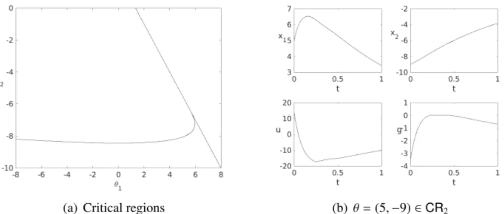
Two critical regions found on application of the algorithm in Sect.3.2are shown in Fig.6(a), where part of the uncertainty domain is discarded due to infeasibility. The structure of the optimal control solutions in the critical regionCR1consist of a unique interior arc, whereas those solutions inCR2are comprised of three
arcs, an interior arc, followed by a boundary arc where the path constraint is binding, and a final interior arc constrained arc sharing the same control law as inCR1. Here, the boundary betweenCR1andCR2consists of those optimal control solutions where the path constraint activates at a single critical point along the time horizon [0,1], and turns out to be nonlinear. For illustration, the optimal control and response trajectories along with the path constraint profile are shown in Fig.6(b)for the uncertainty realizationθ=(5,−9) in the critical regionCR2; the path constraint is active over the time interval [0.2465,0.4205].
(a) Critical regions (b)θ=(5,−9)∈CR2
Figure 6: Optimal solution of the mp-DO problem (27).
4.2. Critical regions in mp-DO problem with second order state constraints
We now consider the following problem:
min u(t),x1(t),x2(t), 0≤t≤1 Z 1 0 1 2u(t) 2dt s.t. " ˙ x1(t) ˙ x2(t) # = " 0 1 0 0 # " x1(t) x2(t) # + " 0 1 # u(t) with " x1(0) x2(0) # = " 0 θ2 # −θ1 ≤x1(t)≤θ1 x1(1)≤0, x2(1)≤θ2, (28)
where the path constraints are of second order. Here, uncertaintyθ∈Θ:=[0,1]×[−1,1] is present both in the initial conditions and the path/terminal constraints.
(a) Critical regions (b)θ(1)=(0.15,0.8)∈CR
2 (c) θ(2)=(0.1,0.8)∈CR4
Figure 7: Optimal solution of the mp-DO problem (28).
A total of five critical regions is obtained for this mp-DO problem on application of the method presented in Sect. 3.2, as shown in Fig. 7(a). It turns out that this partition could in fact be extended to the entire right-half plane {θ1 ≥ 0}. The critical region CR1 corresponds to unconstrained optimal solutions. In CR2 andCR3, the solutions are comprised of two interior arcs separated by a touch-and-go point for the
constraints; this behavior is illustrated for the optimal control solution forθ=(0.15,0.8)∈CR2on Fig.7(b),
where the terminal constraint x1(1) ≤ 0 is also seen to be active. Finally, inCR4 andCR5, the optimal solutions are comprised of three arcs, the first and last ones unconstrained and the middle one binding for the path constraints x1(t) ≤ θ1 and x1(t) ≥ −θ1, respectively; this behavior is illustrated for the optimal
control solution forθ = (0.1,0.8)∈CR4on Fig.7(c), where the path constraintx1(t) ≤ 0.1 remains active along the time interval [0.375,0.625].
4.3. Multi-parametric NCO-tracking control of an FCC unit
This final case study considers a fluidized catalytic cracking (FCC) unit operated in partial combus-tion mode [41]. The objective is to steer the system to a given operating point, defined in terms of the mass fraction of coke on regenerated catalyst,Crc, and the regenerator dense bed temperature, Trg. The manipulated variables are the flow rate of air sent to the regenerator,Fa, and the catalyst flow rate, Fs. A
linear input-output dynamic model is obtained via linearization and reduction of a first-principles nonlinear model around the equilibrium pointCrc∗ = 5.207×10⁻³, Trg∗ = 965.4 K, Tro∗ = 776.9 K, Tcy∗ = 988.1 K, andTf∗ = 400 K, where Tf denotes the feed oil temperature. The control and state variables in this linear
dynamic system are
x(t) := " Crc(t)−C∗rc Trg(t)−Trg∗ # , and u(t) := " Fs(t)−Fs∗ Fa(t)−F∗a # .
The optimization-based control problem is given by
min u(t),x(t),y(t) 1 2x(tf) TQ fx(tf)+ Z 10 0 1 2x(t) TQx(t)+1 2u(t) TRu(t)dt s.t. x˙(t)= Fxx(t)+Fuu(t)+Fθθ3 g(x(t),u(t))≤0 x(0)=(θ1, θ2) (29) with: Qf = " 3.011×10⁷ 1334 1334 1.260 # , Q= " 108 0 0 1 # ,R= " 1 0 0 1 # , Fx = " −2.55×10⁻² 1.51×10⁻⁶ 227 −4.10×10⁻² # ,Fu= " 3.29×10⁻⁶ −2.60×10⁻⁵ −2.8×10⁻² 7.80×10⁻¹ # ,Fθ= " 6.87×10⁻⁷ 2.47×10⁻² # ,
and the path constraintsg(x(t),u(t))≤0 given by:
∀t∈[0,10], " −100 −15 # ≤u(t)≤ " 100 15 # and " −10−3 −20 # ≤ x(t)≤ " 10−3 20 # .
The parametersθin this mp-DO formulation correspond to uncertainty inCrc,Trg, andTf.
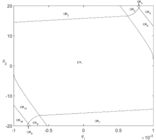
We solve the mp-DO problem (29) with the approach presented in Sect. 3.2, for the uncertainty set
Θ:= [−10−3,10−3]×[−20,20]×[−10,10]. Overall, 11 critical regions are obtained, as shown in Fig.8– both in a 3-d plot (Fig.8(a)) and the corresponding 2-d projections for the parameter valueθ3=0 (Fig.8(b));
the discretized mp-QP counterparts for the latter will be presented later on (Fig.10).
• The critical region CR1 corresponds to unconstrained optimal controls; for instance, the optimal
(a) Full parameter space (b) Projections forθ3=0
Figure 8: Critical regions of the mp-DO problem (29).
• The solutions in bothCR2 andCR7are comprised of two arcs, a boundary arc whereu2 reaches its
lower bound or its upper bound, respectively, followed by an interior arc. This situation is illustrated in Fig.9(b)forθ(2) =(10−4,20,0)∈CR2.
• The solutions in both CR6 and CR11 are comprised of three arcs, with a boundary arc where x1
reaches its upper bound or its lower bound, respectively, located in between an initial interior arc and a final one. In bothCR5andCR10, the solutions have the same constrained arc as CR6 andCR11,
respectively, yet without the final interior arc as the state constraint remains active until the terminal time.
• The solutions inCR3andCR8combine the previous two cases inCR2+CR6orCR7+CR11, and give rise to four arcs, starting with a boundary arc foru2(as inCR2 orCR7), followed by an interior arc,
a boundary arc forx1(as inCR6orCR11), and another interior arc; this case is illustrated in Fig.9(c)
forθ(3)= (6×10−4,20,0)∈CR3. The solutions inCR4andCR9present the same structure asCR3
andCR11, respectively, but lack the final interior arc after the boundary arc wherex1is active.
(a)θ(1)=(5×10−4,5,0)∈CR
1 (b)θ(2)=(10−4,20,0)∈CR2 (c)θ(3)=(6×10−4,20,0)∈CR3
For comparison, the critical regions shown in Fig. 10 are for the discretized mp-QP counterparts of (29) with eitherN = 20 or N = 50 time subintervals and forθ3 = 0. In both cases, the central regions
correspond to unconstrained solutions, likeCR1in Fig.8; all the other critical regions contain one or more
active constraints along certain time subintervals, thereby approximating the six critical regionsCR2-CR11
in Fig.8and the nonlinear feedback control laws thereof in terms of affine control laws only. The actual switching structure gets better approximated as the time discretization is refined, but this also leads to a significant increase in the number of critical regions, namely 175 withN = 20 and 1687 withN = 50. In sum, the comparison with a classical mp-QP approach confirms the clear benefit offered by a continuous-time mp-DO approach in terms of a lesser number of critical regions, along with the ability to capture the underlying nonlinear feedback control nature.
(a) N=20 (b) N=50
Figure 10: Critical regions of discretized mp-QP counterparts of problem (29) forθ3=0.
Closed-loop responses of the FCC unit based on the multi-parametric NCO-tracking controller derived from mp-DO problem (29) are shown in Fig.11, starting from the uncertainty scenario (8×10−4,15,0)∈
CR6att=0. A sampling period of∆T =10−2and signal-to-noise ratios of 50dB (Gaussian white noise) are
considered in both cases, yet with different scenarios for the feed temperature. In the left plot (Fig.11(a)), a nominal feed temperatureT/rm f is used, soθ3=0 at all times; whereas the right plot (Fig.11(b)correspond
to multiple step changes in the value ofθ3as
θ3=0 if 0≤t≤5; θ3 =5 if 5≤t≤10; θ3 =−5 if 10≤t≤15; θ3=0 ift≥15.
The resulting control and response trajectories (solid lines) present a good control performance compared to the nominal case (dashed lines: noise-free and infinite sampling).
5. Conclusions
This paper has introduced a framework for parametric NCO tracking that exploits the multi-parametric solution structure of an uncertain optimal control problem, without the need for applying a time discretization. In the special case of linear-quadratic optimal control problems, an algorithm has been
(a)θ3=0 all the time and 50dB signal-to-noise ratio (b)θ3with step changes and 50dB signal-to-noise ratio
Figure 11: Closed-loop response of the multi-parametric NCO-tracking controller for problem (29).
proposed for characterizing the corresponding multi-parametric solution structure in terms of the exact critical regions and nonlinear feedback control laws. In practice, these feedback laws can be applied in a receding horizon manner, effectively resulting in a closed-loop, multi-parametric NCO-tracking controller for the system. In comparison to classical NCO tracking, this approach no longer requires the assumption of an invariant active set in the presence of uncertainty and extends the scope of NCO tracking to receding horizon control; whereas addressing the uncertain optimal control problem in its native, continuous-time form may lead to a dramatic reduction in the number of critical region compared to the classical mp-QP approach based on time discretization, due to the ability to capture the underlying nonlinear feedback control nature. These properties have been illustrated with several examples throughout the paper, including the two-input control problem of an FCC unit. Future work will focus on an extension of this approach to addressing (certain classes of) nonlinear systems.
Acknowledgments. M. Sun is grateful to the Department of Chemical Engineering and the Faculty of Engi-neering of Imperial College London for an EPSRC International Doctoral Training Award (DTA). Financial support from Texas A&M University and from the Centre of Process Systems Engineering (CPSE) of Im-perial College is also gratefully acknowledged.
References
[1] S. S. Bahakim, L. A. Ricardez-Sandoval, Simultaneous design and MPC-based control for dynamic systems under uncer-tainty: A stochastic approach, Computers & Chemical Engineering 63 (2014) 66–81.
[2] J. B. Rawlings, D. Q. Mayne, Model Predictive Control: Theory and Design, Nob Hill Publishing, 2009.
[3] E. N. Pistikopoulos, From multi-parametric programming theory to MPC-on-a-chip multi-scale systems applications, Com-puters & Chemical Engineering 47 (2012) 57–66.
[4] V. Sakizlis, J. D. Perkins, E. N. Pistikopoulos, Explicit solutions to optimal control problems for constrained continuous-time linear systems, IEE Proceedings: Control Theory and Applications 152 (4) (2005) 443–452.
[5] E. N. Pistikopoulos, M. C. Georgiadis, V. Dua, Multiparametric programming: Theory, algorithms and applications, Wein-heim: Wiley-VCH, 2007.
[6] E. N. Pistikopoulos, Perspectives in multiparametric programming and explicit model predictive control, AIChE Journal 55 (2009) 1918–1925.
[7] E. N. Pistikopoulos, L. Dominguez, C. Panos, K. Kouramas, A. Chinchuluun, Theoretical and algorithmic advances in multi-parametric programming and control, Computational Management Science 9 (2) (2012) 183–203.
[8] E. N. Pistikopoulos, N. A. Diangelakis, R. Oberdieck, M. M. Papathanasiou, I. Nascu, M. Sun, PAROC - an integrated framework and software platform for the optimisation and advanced model-based control of process systems, Chemical Engineering Science 136 (2015) 115–138.
[9] A. Bemporad, M. Morari, V. Dua, E. N. Pistikopoulos, The explicit linear quadratic regulator for constrained systems, Auto-matica 38 (2002) 3–20.
[10] L. F. Dominguez, E. N. Pistikopoulos, Recent advances in explicit multi-parametric nonlinear model predictive control, Industrial & Engineering Chemistry Research 50 (2011) 609–619.
[11] H. J. Pesch, Real-time computation of feedback controls for constrained optimal control problems part 1: Neighboring extremals, Optimal Control Applications & Methods 10 (2) (1989) 130–145.
[12] K. Malanowski, H. Maurer, Sensitivity analysis for parametric control problems with control-state constraints, Computational Optimization & Applications 5 (1996) 254–283.
[13] K. Malanowski, H. Maurer, Sensitivity analysis for state constrained optimal control problems, Discrete & Continuous Dy-namical Systems 4 (2) (1998) 241–272.
[14] K. Malanowski, H. Maurer, Sensitivity analysis for optimal control problems subject to higher order state constraints, Annals of Operations Research 101 (2001) 43–73.
[15] H. Maurer, H. J. Pesch, Solution differentiability for parametric nonlinear control problems with control-state constraints, Journal of Optimization Theory & Applications 86 (2) (1995) 285–309.
[16] D. Augustin, H. Maurer, Computational sensitivity analysis for state constrained optimal control problems, Annals of Oper-ations Research 101 (2001) 75–99.
[17] A. E. Bryson, Y. Ho, Applied Optimal Control, Wiley, New York, 1975.
[18] E. Kreindler, Additional necessary conditions for optimal control with state-variable constraints, Journal of Optimization Theory & Applications 38 (2).
[19] R. F. Hartl, S. P. Sethi, R. Vickson, A survey of the maximum principle for optimal control problems with state constraints, SIAM Review 37 (1995) 181–218.
[20] J. V. Kadam, M. Schlegel, B. Srinivasan, D. Bonvin, W. Marquardt, Dynamic optimization in the presence of uncertainty: From off-line nominal solution to measurement-based implementation, Journal of Process Control 17 (2007) 389–398. [21] D. Bonvin, B. Srinivasan, On the role of the necessary conditions of optimality in structuring dynamic real-time optimization
schemes, Computers & Chemical Engineering 51 (2013) 172–180.
[22] G. Franc¸ois, B. Srinivasan, D. Bonvin, Use of measurements for enforcing the necessary conditions of optimality in the presence of constraints and uncertainty, Journal of Process Control 15 (2005) 701–712.
[23] A. Grancharova, T. Johansen, P. Tøndel, Computational aspects of approximate explicit nonlinear model predictive control, in: R. Findeisen, F. Allgower and L. Biegler, eds. Assessment and Future Directions of Nonlinear Model Predictive Control, Springer, 2007, pp. 3181–192.
[24] E. N. Pistikopoulos, M. C. Georgiadis, V. Dua, Multi-parametric model-based control: Theory and applications, Weinheim: Wiley-VCH, 2007.
[25] B. Srinivasan, D. Bonvin, E. Visser, S. Palanki, Dynamic optimization of batch processes: II. Role of measurements in handling uncertainty, Computers & Chemical Engineering 44 (2003) 27–44.
[26] M. Schlegel, W. Marquardt, Detection and exploitation of the control switching structure in the solution of dynamic opti-mization problems, Journal of Process Control 16 (2006) 275–290.
[27] B. Srinivasan, D. Bonvin, Real-time optimization of batch processes by tracking the necessary conditions of optimality, Industrial & Engineering Chemistry Research 46 (2007) 492–504.
[28] B. Srinivasan, D. Bonvin, Dynamic optimization under uncertainty via NCO tracking: A solution model approach, BatchPro Symposium Plenary talk (2004) 17–35.
[29] S. Gros, B. Srinivasan, D. Bonvin, Optimizing control based on output feedback, Computers & Chemical Engineering 33 (2009) 191–198.
[30] S. Gros, B. Srinivasan, B. Chachuat, D. Bonvin, Neighboring-extremal control for singular dynamic optimization problems. I – Single-input systems, International Journal of Control 82 (6) (2009) 1099–1112.
[31] S. Gros, B. Srinivasan, B. Chachuat, D. Bonvin, Neighboring-extremal control for singular dynamic optimization problems. II – Multiple-input systems, International Journal of Control 82 (7) (2009) 1193–1211.
[32] K. B. Ariyur, M. Krstic, Real-Time Optimization by Extremum-Seeking Control, Wiley, 2003.
[33] D. Dochain, M. Perrier, M. Guay, Extremum seeking control and its application to process and reaction systems: A survey, Mathematics & Computers in Simulation 82 (2011) 369380.
[34] S. A. Deshpande, D. Bonvin, B. Chachuat, Directional input adaptation in parametric optimal control problems, SIAM Journal on Control and Optimization 50 (4) (2012) 19952024.
[35] D. Bonvin, B. Srinivasan, D. Hunkeler, Control and optimization of batch processes, IEEE Control Systems Magazine 26 (6) (2006) 34–45.
[36] P. Brunovsk´y, Regular synthesis for the linear-quadratic optimal control problem with linear control constraints, Journal of Differential Equations 38 (3) (1980) 344–360.
[37] C. Bruni, D. Iacoviello, A study on abnormality in variational and optimal control problems, Journal of Optimization Theory & Applications 121 (2004) 41–64.
[38] B. Chachuat, B. Houska, R. Paulen, N. Peri´c, J. Rajyaguru, M. E. Villanueva, Set-theoretic approaches in analysis, estimation and control of nonlinear systems, IFAC-PapersOnLine 48 (8) 2015 981–995.
[39] L. T. Biegler, Nonlinear Programming: Concepts, Algorithms and Applications to Chemical Processes, MOS-SIAM Series on Optimization, 2010.
[40] M. Schlegel, W. Marquardt, Adaptive switching structure detection for the solution of dynamic optimization problems, In-dustrial & Engineering Chemistry Research 45 (24) (2006) 8083–8094.
[41] M. Hovd, S. Skogestad, Procedure for regularity control structure selection with application to the FCC process, AIChE Journal 39 (12) (1993) 1938–1953.
Appendix A. Feedback law derivation for the illustrative example
We follow the steps presented in Sect.3.2.3in order to determine the critical regions in the uncertainty domainΘ:=[−2,2]2.
• We start with the pointθ=(0,0), whose corresponding optimal control solution is unconstrained. We denote byS(1)this solution structure, which is comprised of a single arc (Nt(1) =1). Expressions for the state and adjoint trajectories as a function ofθare obtained directly from (22), with the missing initial adjoints determined from (24) as
" x(t0) p(t0) # = 1 0 0 1 1.6396 1.6396 1.6396 21.6396 θ .
An expression ofu(t) follows from (19) as
u(t, θ)=h−8.198 −8.198iθexp(−10.198t), (A.1)
Finally, an implicit characterization of the critical region CR(1) corresponding to S(1) is obtained
from (26) which, in the absence of active constraints, corresponds to values ofθfor which both input constraints remain inactive:
CR(1) := ( θ∈[−2,2]2 " 1 1 −1 −1 # θ≤ " 0.2440 0.2440 # ) .
• The pointθ = (1,1) happens to be in the uncertainty domain Θ, yet outside CR(1). The structure
S(2)of the optimal control at this point is comprised of two arcs (Nt(2) = 2), namely a boundary arc corresponding to an active lower input bound, followed by an interior arc. The determination of an explicit feedback control law starts by computing the adjoint initial conditionp(t0) as a function ofθ
from (24), then expressing the state/co-state trajectories as a function ofθby (22), and finally using (19). In this specific case, an explicit expression of the switching time functiont1(θ) can be obtained by expressing continuity of the optimal control att1as
and an expression of the feedback controlu(t) is given by u(t, θ)= −2, ift≤t1(θ) −2 exp(−18.396[t−t1(θ)]), otherwise
An implicit characterization of this critical region is obtained from (26) as CR(2) := nθ∈[−2,2]2 h −1 −1iθ≤ −0.2440o.
• The pointθ = (−1,−1) happens to be in the uncertainty domainΘ, yet outside CR(1)∪CR(2). The structureS(3)of the optimal control at this point is also comprised of two arcs (N(3)
t = 2), namely a boundary arc corresponding to an active upper input bound, followed by an interior arc. The determi-nation of an explicit feedback control law and the characterization of CR(3)are similar to the previous case: u(t, θ)= 2, ift≤t1(θ) 2 exp(−18.396[t−t1(θ)]), otherwise witht1(θ)=0.5 ln(0.8039(1−θ1−θ2)), and CR(3) := nθ∈[−2,2]2 h 1 1iθ≤ −0.2440o.
• At this point, we have CR(1)∪CR(2)∪CR(3) = Θand the procedure terminates with a total of three critical regions.