Infinite-Term Memory Classifier for Wi-Fi
Localization Based on Dynamic Wi-Fi Simulator
AHMED SALIH AL-KHALEEFA 1, MOHD RIDUAN AHMAD1,
AZMI AWANG MD ISA1, (Member, IEEE), MONA RIZA MOHD ESA2,
AHMED AL-SAFFAR3, AND YAZAN ALJEROUDI4
1Broadband and Networking Research Group, Centre for Telecommunication and Research Innovation, Fakulti Kejuruteraan Elektronik dan Kejuruteraan
Komputer, Universiti Teknikal Malaysia Melaka, Durian Tunggal 76100, Malaysia
2Institute of High Voltage and High Current, School of Electrical Engineering, Faculty of Engineering, Universiti Teknologi Malaysia, Skudai 81310, Malaysia 3Faculty of Computer System and Software Engineering, Universiti Malaysia Pahang, Gambang 26300, Malaysia
4Department of Mechanical Engineering, International Islamic University of Malaysia, Gombak 53100, Malaysia
Corresponding author: Ahmed Salih Al-Khaleefa ([email protected])
This work was supported by the Malaysia Ministry of Education, Universiti Teknikal Malaysia Melaka, under Grant PJP/2018/FKEKK(3B)/S01615, and in part by Universiti Teknologi Malaysia under Grants 14J64 and 4F966.
ABSTRACT Wi-Fi localization is an active research topic, and various challenges are not yet resolved in this field. Researchers develop models and use benchmark datasets for Wi-Fi or fingerprinting to create a quantitative comparative evaluation. These benchmarking datasets are limited by their failure to support dynamical navigation. As a result, Wi-Fi models are only evaluated as usual classifiers without including actual navigation maneuvers in the evaluation, which makes the models incapable of handling the actual navigation behavior and its impact on the performance. One common navigation behavior is the cyclic dynamic behavior, which occurs frequently in the indoor environment when a person visits the same place or location multiple times or repeats the same trajectory or similar one more than once. For this purpose, we developed two models: a simulation model for generating time series data to support actual conducted navigation scenarios and a Wi-Fi classification model to handle dynamical scenarios generated by the simulator under cyclic dynamic behavior. Various testing scenarios were conducted for evaluation, and a comparison with benchmarks was performed. Results show the superiority of our developed model which is infinite-term memory online sequential extreme learning machine (OSELM) to the benchmarks with a percentage of 173% over feature adaptive OSELM and 1638% over OSELM.
INDEX TERMS Indoor localization, extreme learning machine, Wi-Fi cyclic dynamics, feature adaptive.
I. INTRODUCTION
Indoor localization or indoor positioning systems (IPSs) are considered non-fully resolved research problems. Different technologies, such as personal dead reckoning (PDR) [1] and wireless-based systems [2], have been used for IPS. Wireless local area networks (WLANs), which are collectively known as Wi-Fi technology, are widespread and readily available to enable and support broadband communications. Wi-Fi-based positioning, particularly indoor Wi-Fi-Wi-Fi-based position-ing, is a mature positioning technology due to its simplicity, ease of access to Wi-Fi received signal strength (RSS) mea-surements on various devices and systems, and low cost of implementation. Considerable research has been dedicated to Wi-Fi-based indoor positioning. Surveys on this topic can be found in [3].
The research community recognizes that Wi-Fi-based posi-tioning can reach an accuracy down to a few meters. However, available benchmarking datasets for Wi-Fi-based position-ing are limited. Most researchers use them in conventional machine learning scheme for training and testing. This usage is useful for testing localization performance under static scenarios. The practical installation of systems includes the dynamical aspect that is essential in driving the localization prediction. Therefore, a valuable benchmarking must support the generation of data depending on the entire navigation scenario.
Some researchers [4] argued that the four factors below hinder the objective evaluation of existing Wi-Fi-based IPSs: • Non-standardized measurement spaces: Studies have measured spaces ranging from one or two rooms to
multi-floor, multi-corridor, or even multiple multi-story buildings.
• Non-standardized conventions regarding stored data: Works have focused on storing the RSS of heard access points (APs) in a certain measurement point (dBm ver-sus linear scale and conventions for non-heard AP), determining the number of RSS and AP values to store per measurement point (all heard versus some truncation rules), and deciding on the number of times the measure-ments should be collected and which spacing or grid to use.
• Non-standardized localization hardware: Studies have considered different AP models and many possible strategies to deploy the Wi-Fi network infrastructure. • Non-unified understanding regarding the available data:
Researchers have dedicated efforts on treating a heard AP over multiple floors (separately, per floor, or in a 3D space) and interpreting data stored by floors with missing height dimension.
Such factors have been resolved by providing open source datasets [4]. Nevertheless, an important factor can be added to the limitation of using datasets as benchmarking for develop-ment. This factor is the static nature of the provided dataset, which prevents its utilization by the developer for evaluating dynamical scenarios of its IPS.
The actual nature of mobility of people in an indoor ronment is its dynamical aspect. People in an indoor envi-ronment have the following features as reflected by their recorded trajectories:
1- These people have cyclic dynamic nature. Specifically, when a person goes from one place to another, he or she may return to the previous place. Going back and forth is also a general behavior of these people. For example, a person in an office area goes to the restroom or another office in the building.
2- The velocity of the moving person is not constant and varies within certain range. This condition brings addi-tional dynamics to the trajectory.
3- Certain segments of the path are repeated. For example, using corridors requires a person to go from the same segment in the going and returning directions.
The above-mentioned characteristics bring difficulty to the classifier during classification. Specifically, the APs that are used for feeding the classifier with features will change in number. This change is due to the limited range of one AP; accordingly, some APs will go out of the range, and others will enter the range of the Wi-Fi sensor. As a result, the classical learning classifiers, such as OSLEM, will not be effective anymore. Several researchers have aimed to address this matter by using adaptive feature classifiers, such as FA-OSELM, which create a new neural network and perform transfer learning when the number of features changes. The transfer learning is responsible of transferring the knowledge from the old to the new neural network. However, these classifiers cannot restore the old knowledge from previous
neural networks when a person visits an early visited place. The contributions of this study are summarized as follows:
1- An approach for extending the available datasets for benchmarking Wi-Fi localization and making it sup-portive to dynamical scenarios for evaluation is pro-posed.
2- An extreme learning-based classifier that can perform two functions, namely, transfer learning when the num-ber of features changes and restoring old knowledge if needed, is proposed.
3- The simulator and the developed classifier are evaluated on the basis of state-of-the-art approaches.
The remainder of the article is organized as follows. Section 2 provides the literature review. Section 3 presents the needed background. Section 4 presents the developed methodology, and Section 5 shows the experimental results and evaluation. Finally, Section 6 gives the summary and conclusion.
II. LITERATURE REVIEW
The literature review contains two subsections. Subsection A provides a review of the existing fingerprint datasets in lit-erature. Subsection B presents a review of previous machine learning approaches for solving Wi-Fi localization.
A. FINGERPRINT DATASETS
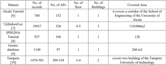
Literature contains several datasets that have been collected as fingerprint to help researchers in Wi-Fi localization. These datasets differ in sizes, dimensions, covered space, and the nature of the studied building. Some datasets are collected in corridor-type environments [4]. Other datasets include sev-eral floors [5]. Some datasets contain a combination of single buildings [6], whereas others contain a combination of multi-ple buildings [7]. The number of APs installed in the building also differs from one dataset to another. Table 1 presents a quantitative comparison of frequently used datasets as bench-marking for Wi-Fi localization.
The problem with these datasets is that they cannot sup-port dynamical scenarios. Researchers usually partition the dataset into parts: training, validation, and testing parts. In such case, the location prediction is evaluated on the basis of the partitioning. However, Wi-Fi localization has a dynamic nature, and the trajectory of the moving person with respect to time affects the predicted location. Therefore, the dataset must be arranged as time series depending on the mobility of the user for realistic and practical classification.
Some researchers have developed channel models for Wi-Fi antenna to generate fingerprint data based on simula-tion. This way provides high possibility of evaluating differ-ent scenarios and characterizing the localization model from different aspects and factors related to the number of APs, its distribution, and the geometry of the building [11].
From the literature review, we can conclude that no work on Wi-Fi localization has been conducted to generate time series data of APs under different mobility scenarios.
TABLE 1. Quantitative description of different Wi-Fi datasets in literature.
Such model will make the empirical dataset useful for evalu-ating Wi-Fi localization models.
Several datasets for Wi-Fi localization are avail-able [4], [7]. Such benchmarks are useful as benchmark evaluation for different approaches developed for solving Wi-Fi localization. However, they are limited in the number of the scenarios to be tested. Specifically, when a user wants to evaluate scenarios with a dynamic nature, such as frequent mobility among several areas or any other scenario that includes cycles, the data should be in time series order. To generate such time series from the benchmarks, a simu-lator that accepts scenarios defined by the user and translates these scenarios to trajectory of features (i.e., time series) on the basis of the original benchmark data must be developed. In such case, the simulator will provide realistic data and resolve the static nature of the published data because data for unlimited number of dynamical scenarios can be generated.
Our developed simulator will be based on UJIIndoor-Loc and TampereU. The UJIIndoorUJIIndoor-Loc database comprises three buildings of Universitat Jaume I that have at least four levels with areas of nearly 110.000 m2 [7]. This database can be utilized for classification purposes, such as regression or actual floor and building identification and actual estimation of longitude and latitude. UJIIndoorLoc was developed in 2013 with over 20 distinct users and 25 Android devices. The database consists of 1,111 val-idation/test records and 19,937 training/reference records. A total of 529 attributes all have the Wi-Fi fingerprint, includ-ing the coordinates of where the information was obtained, and other relevant information.
The TampereU dataset is an indoor localization database used for testing IPSs that are dependent on the WLAN/Wi-Fi fingerprint. The database was created by Cramariuc and Lohan [10] for testing indoor localization techniques. Tam-pereU incorporates two buildings of the Tampere Uni-versity of Technology that have three and four levels, respectively. The database contains 489 test attributes
and 1,478 training/reference records of the first build-ing, and 312 attributes of the second building. The coordinates (latitude, longitude, and height) and the Wi-Fi fingerprint (309 WAPs) are also contained in this database.
B. MACHINE LEARNING APPROACHES FOR SOLVING WI-FI LOCALIZATION
Numerous machine learning algorithms, such as OSELM [12], have been used for Wi-Fi localization. OSELM has a fast learning speed that can lessen manpower and time costs associated with the offline site survey. This algorithm pos-sesses an online sequential learning ability that allows the proposed localization algorithm to adapt to the environmen-tal dynamics in a timely and automatic manner. Weighted extreme learning machine has also been integrated with signal tendency index for Wi-Fi-based localization on the basis of standardized fingerprint. In [13], two types of robust extreme learning machines (RELMs), small-residual and close-to-mean constraints, are proposed to address noisy measurement issues in IPSs. Their performance depends on the explicit feature mapping in the extreme learning machine. Second-order cone programming is used to provide random hidden nodes and kernelized RELM formulations. These methods have been applied to indoor Wi-Fi localization and offer higher accuracy than the basic ELM. In [14], ELM is utilized for a transfer learning framework. The developed framework can remove or add APs to the environment, thereby leading to changes in the fingerprint model. Transfer learning is utilized for the neural network to adapt to a new situation without collecting the new fingerprint. The old information obtained within the neural network may be moved to the new network with the assistance of two matrices for the input weight transfer matrix and an input weight supplement vector. The latter will aid the system to undertake the required adjust-ments concerning the evolving dimension of feature matrices among the domains along with online sequential learning.
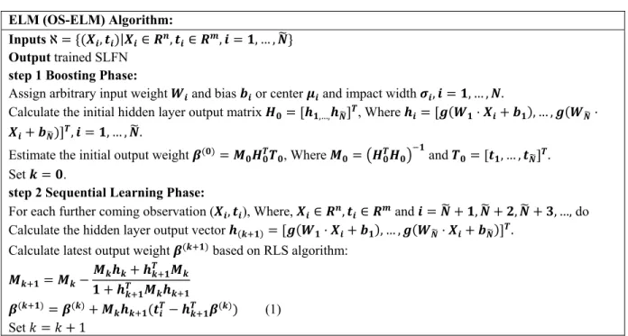
TABLE 2. Procedure of OSELM training.
This model is useful for avoiding traditional and exhaust-ing trainexhaust-ing processes when an expected update occurs in the data distribution because of domain or environmental changes. However, the model suffers from losing all the old knowledge and information acquired from the network. This knowledge is important when a high dynamical change occurs in the environment, which drives the restoration of the old knowledge in the system when another change occurs. One specific example regarding Wi-Fi localization is when users travel back and forth in areas of an indoor environment.
III. BACKGROUND
This section provides the needed background for our devel-oped ITM-OSELM. Subsections A and B present an overview of OSELM and FA-OSELM, respectively.
A. OSELM REVIEW
Data are unavailable in advance for a broad range of applica-tions. Instead, data are continuously generated with respect to time. Thus, each time a new block becomes available, training on the block of data is needed. In [15], a mathemat-ical method to perform online sequential learning for ELM called OSELM is developed. OSELM involves two main phases. In the boosting phase, SLFNs are trained using the primitive ELM method along with some batches of training data used in the initialization stage. After the boosting phase is completed, the training data in this phase are discarded. Then, OSELM learns the training data by chunks or indi-vidually. After the data are trained, all of them are dis-carded. The procedure of the OSELM algorithm is presented in Table 2.
B. FA-OSELM REVIEW
FA-OSELM [14] transfers old knowledge to a new network from a pre-trained neural network when the number of fea-tures between the two networks differs. If same amounts of hidden nodesLare available, then FA-OSELM offers an input weight supplement vectorQi and an input weight transfer matrixPto move to the new weighta0ifrom the old weightsai. To perform this task, FA-OSELM uses the equation that considers that the amount of feature changes frommttomt+1.
{a0i=ai·P+Qi}Li=1, (2) where P= P11 · · · P1mt+1 ... ... ... Pmt1 · · · Pmtmt+1 mt×mt+1 (3) Qi =[Q1 . . . Qmt+1]1×mt+1. (4)
Matrix P must obey the following rules:
• Each line has only one ‘‘1’’, and the rest of the lines has all ‘‘0’’.
•Each column has only one ‘‘1’’ at most, and the rest of the lines has all ‘‘0’’.
•Pij =1 indicates that, after a change in the feature dimen-sion, the ith dimension for the original feature vector will become thejthdimension for the new feature vector. When the feature dimension increases,Qiwill serve as the supplement. The corresponding input weight is also added for the newly added features. Moreover, the following rules serve as part ofQi.
FIGURE 1. Wi-Fi-SCD simulator architecture and its sub-blocks.
•Low feature dimensions indicate thatQican be considered an all-zero vector. Thus, no additional corresponding input weight is needed by the newly added features.
•If the new feature is represented by theithitem ofa0iwhen feature dimension increases, then a random generation of the ith item of Qi should be conducted on the basis of the ai distribution.
IV. METHODOLOGY
This section provides the developed method of building sim-ulator for dynamical scenarios based on benchmark finger-print. Subsection A presents the simulator architecture, and Subsection B gives the detailed procedure of the simulation. Subsection C discusses the developed ITM-OSELM archi-tecture, and Subsection D provides the algorithmic part of ITM-OSELM. Finally, Subsection E presents the evaluation measures.
A. SIMULATOR ARCHITECTURE
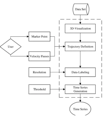
The simulator is composed of four blocks: 3D visualization, trajectory definition, data labeling, and time series genera-tion. Each of the blocks provides an input to the subsequent block. A block diagram of the sequential relation among the blocks is shown in Fig. 1. The 3D visualization block determines the measurement points of the fingerprint of the environment in 3D geometrical plot. With this visualization, the user can estimate the trajectory that he or she will provide to the system. The trajectory is represented under three types of information: marker points that refer to the stop points in the trajectory, velocities that refer to the average velocity between two marker points, and pauses that refer the stopping
period at each marker point. The trajectory definition block processes the trajectory information and generates the time series of point data that will be used for data labeling under the provided resolution or grid granularity. The time series generation block produces the features data with the labels. This block uses the threshold parameter that represents the radius of the circle. With this circle, the APs that can be sensed from certain location can be determined. Therefore, the final time series data are labeled depending on the defined resolution and contain features depending on the sensed APs in each location.
These data are generated on the basis of the actual charac-teristics of the navigated trajectory with respect to velocities and pauses. Fig. 2 shows two examples of data visualization from TampereU and UJIndoorLoc. Fig. 3 shows the final generated trajectory depending on user input in one and two floors.
B. PROCEDURE OF WI-FI SIMULATOR FOR CYCLIC DYNAMICS
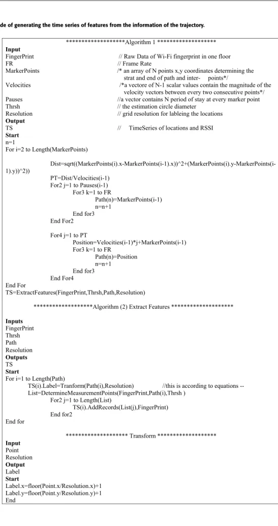
We aim to convert the predefined trajectory to time series of features with their corresponding labels depending on the number of APs in each point of the path. The gen-erated records of the time series are dependent on the velocity of the moving person. The algorithm of this generation is called Wi-Fi simulator for cyclic dynamics (Wi-Fi-SCD).
To achieve this goal, the trajectory will be provided through three parts of information: the marker point vector, which represents the location of the stop points of the trajectory; the velocity vector, which represents the velocity vector between two marker points; the pauses, which represent the time period for each stop in the trajectory. The frame rate of the Wi-Fi sensor is regarded as an input to the algorithm. The algorithm will use this information to generate time series of the locations that the person has visited while moving. In each location, the Wi-Fi sensor will sense a set of APs to provide RSSI to the features of the record. The variable Thrsh is used to determine the sensed AP in certain location. This variable represents the radius of sensing of the Wi-Fi sensor. All the measurement points inside the fingerprint will be used as markers to include the RSSI of their APs inside the record of this location. The mathematical model of building the time series is given in Equations (5)–(8).
PTi =
dist(mpi−1,mpi)
vi
(5)
i=1,2. . .N, whereNdenotes the number of marker points
N1 =FR×Ti (6)
pt =vt+pt−1 (7)
N2 =FR (8)
wherempidenotes the marker points of the stop points dur-ing the path provided by the user,vi denotes the velocities between two stop points,Ti denotes the time of pauses at
FIGURE 2. Fingerprint of multiple floors (measurement points) from (a) TampereU and (b) UJIndoorLoc.
FIGURE 3. Simulated trajectory in (a) multiple floors and (b) single floor.
the stop points, FR denotes the frame rate of the sensors, N1 represents the number of repeating the point of the pause in the time series, and N2 represents the number of repeating any point pt of the trajectory in the time series within a period of 1 s. After the points of the time series are generated, they will be transformed to new coordi-nate system depending on the defined resolutions by using Equations (9)–(10). xi0 = b xi Res.xc +1, (9) y0i = y i Res.y +1, (10)
where Res.x and Res.y represent the grid granularity. The pseudocode that describes this algorithm is presented in Table 3.
C. ARCHITECTURE OF ITM-OSELM
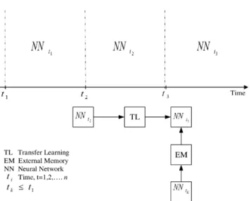
ITM-OSELM is a novel variant of OSELM and is presented to address the problem of knowledge loss. ITM-OSELM is composed of two blocks: one is transfer learning similar to that of FA-OSELM, and the other is external memory. The transfer learning block (TL block) transfers the knowledge from the old network to the new network when the number of features changes. This procedure is useful to avoid the knowledge loss in OSELM when some APs disappear and others appear. The external memory block (EM block) stores the weights related to the features that become disabled at certain point of time t. Whenever the features are active again, the EM block will provide the classifier with the weights related to these features. As a result, the classifier gains initial knowledge from the EM block to perform effectively. Consid-ering that the classifier has already gained knowledge from
FIGURE 4. Block diagram of the operation of ITM-OSELM with respect to time.
the TL block, the EM block will complement this knowledge because the TL block is using the previous classifier to feed the EM block. However, the previous classifier does not contain any knowledge related to the new active features. Therefore, the EM block is needed to restore this knowledge. A block diagram to explain the concept of ITM-OSELM is provided in Fig. 4. Notably, the neural network is evolving at certain time pointst1,t2,t3. . .when the number of features changes. At each moment of changetk, a new neural network
NNtk will receive knowledge from two sources: one is the TL
block that will capture the needed knowledge fromNNtk−1,
and the other is the EM block that will capture the needed knowledge from old neural networkNNtj, wheretj≤tk−1.
The structure of the EM block is depicted in Fig. 5. The EM block is represented by a matrix with an input size denoted as N, which represents the total number of features in the sys-tem; and a number of columns denoted as L, which represents the number of hidden neurons in the classifier. The memory will be updated only when the number of features changes through storing the values of the weights of the features that become non-active. The memory will also be used when the number of features changes to initialize the classifiers with the weights of the features that become active.
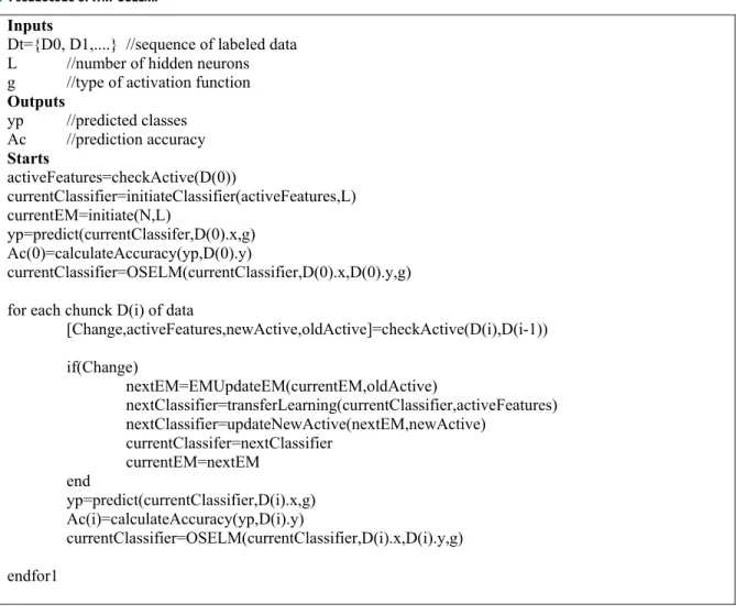
D. ITM-OSELM ALGORITHM
The pseudocode of ITM-OSELM is presented in Table 4. The data are received as chunks or blocks denoted as
Dt = {D0,D1, . . .}. The algorithm receives two types of
information about the setting of the neural network that will operate: one isL, which represents the hidden number of neu-rons; the other isg, which represents the activation function. The output of the pseudocode is the predicted classes at each moment of prediction and the resulted accuracy that will be calculated once the labels of the data are given. From a Wi-Fi localization perspective, the person will use the AP values to predict where he or she exists. The actual location of the person can be determined in future moments. Thus, the neural
FIGURE 5. Representation of the EM block in ITM-OSELM.
network will use the ground truth as labels for updating the knowledge. The pseudocode indicates that, when the number of features changes, the following processes occur: update of the EM block for the old active features, transfer learning from the previous neural network for the same active features, and update from the EM block for the old active features. E. EVALUATION SCENARIOS
Two datasets, namely, TampereU and UJIndoorLoc, are used to evaluate our approach. Two scenarios are generated for the two datasets: The first one is one-floor scenario which is (rectangular) scenario and the second one is multi-floor scenario which is (cubic) scenario. WiFi-SCD will be used for generating the different trajectory scenarios. After the time series are generated, they can be validated using machine learning models. We use online learning models because of the sequential nature of the data available. OSELM is a typi-cal model for sequential learning. However, OSELM creates a new neural network every time new APs are sensed or old APs are lost. This procedure may cause some loss of old knowl-edge. By contrast, FA-OSELM preserves fair amount of old knowledge through knowledge transferring from the old to the new neural network. Thus, OSELM and FA-OSELM are used as benchmarks for comparison with our ITM-OSELM. The trajectories that are generated from the three models will be compared with ground truth. The trajectory will be repre-sented for visualization in graphs, where the nodes represent the location and the edges represent the transition between edges.
Two main measures are generated: the accuracy of each of the calls of testing and training of chunk of data, and the correlation between the predicted path and the ground truth. A high correlation indicates improved performance of the model.
V. EXPERIMENTAL RESULTS AND EVALUATION
ITM-OSELM and Wi-Fi-SCD were evaluated using two datasets: TampereU and UJIIndoorLoc. As stated earlier, our aim was to evaluate the Wi-Fi localization model based on
TABLE 4. Pseudocode of ITM-OSELM.
TABLE 5. Types of the conducted trajectories and their settings for TampereU and UJIIndoorLoc.
dynamical scenarios. Therefore, actual trajectories were gen-erated using the Wi-Fi-SCD, and they were used for training and testing on ITM-OSELM. Two benchmarks were used for comparison: FA-OSELM and OSELM. The generated trajectories are rectangular and cubic. The average velocity of the moving person is 0.3 m/s. The time of pauses is 1 s. Every path was repeated for three times to show the repeatability of the experiment. Table 5 shows the configurations of the scenarios.
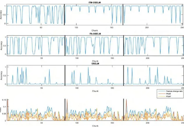
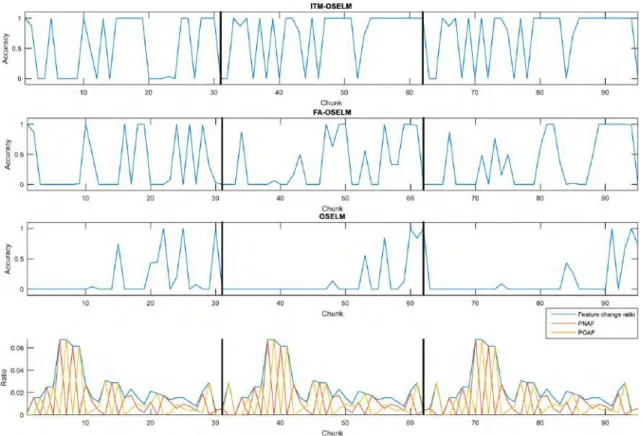
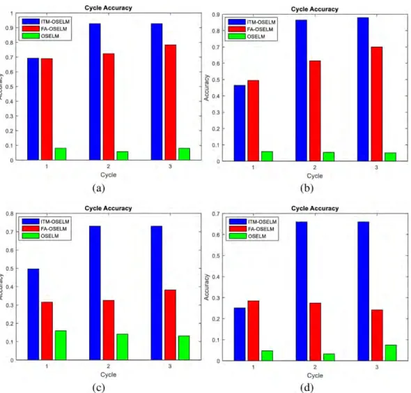
We calculated the prediction accuracy of the scenario with respect to each chunk of data. Figs. 6–9 show the results. The accuracy in each cycle was plotted (Fig. 10) to determine the improvement from one cycle to another. We plotted all figures for ITM-OSELM, FA-OSELM, and OSELM.
From the results, the following observations are obtained: 1. In the first cycle, ITM-OSELM and FA-OSELM show similar performance in accuracy. This trend is general for all evaluation scenarios.
2. In the first cycle, OSELM performs worse than the two other models. The reason is that OSELM lacks any transfer learning capability.
3. For all scenarios, ITM-OSELM shows an increasing trend in accuracy from one cycle to the subsequent one. This performance is due to its knowledge preservation capability, which is lacking in FA-OSELM.
4. For some scenarios, FA-OSELM exhibits an increasing trend in accuracy from one cycle to the subsequent one. By contrast, it shows a decreasing trend in accuracy for other scenarios. This inconsistency is attributed to that the number of features changes with the change in mobility of the person. In other words, if the last neural network of one cycle is useful in transferring its weights as initial weights to the first model in the subsequent cycle, then the accuracy will increase in the second cycle.
We generated the improvement percentage of ITM-OSELM over FA-ITM-OSELM and ITM-OSELM in the last cycle with
FIGURE 6. Accuracy on data chunks for rectangular scenario and the corresponding FCR, PNAF, and POAF with TampereU dataset.
FIGURE 8. Accuracy on data chunks for rectangular scenario and the corresponding FCR, PNAF, and POAF with UJIndoorLoc dataset.
FIGURE 10. Accuracy of the models in cycles with two trajectories and two datasets (a) Rectangular trajectories with TampereU dataset (b) Cubic trajectories with TampereU dataset (c) Rectangular trajectories with UJIndoorLoc dataset (d) Cubic trajectories with UJIndoorLoc dataset.
FIGURE 11. Improvement percentage of ITM-OSELM over FA-OSELM in the last cycle for cubic and rectangular scenarios with TampereU and UJIndoorLoc datasets.
TampereU and UJIndoorLoc for summarizing the results as it shown in Figs. 11 and 12.
Evidently, the developed ITM-OSELM model shows improvement over the two benchmarks for all conducted
FIGURE 12. Improvement percentage of ITM-OSELM over OSELM in the last cycle for cubic and rectangular scenarios with TampereU and UJIndoorLoc datasets.
scenarios with the two datasets. Fig. 11 shows that ITM-OSELM obtains an improvement percentage of 173% over FA-OSELM for cubic scenario with UJIndoorLoc dataset. Fig. 12 shows that ITM-OSELM obtains an improvement
FIGURE 13. Predicted graphs and ground truth represented in graphs for rectangular scenario with TampereU dataset.
percentage of 1638% over OSELM for cubic scenario with TampereU dataset.
For further evaluation, the geometry of the trajectories was compared with the ground truth to investigate the cor-rectness of the prediction from the localization perspective. Figs. 13–16 show the predicted paths for our devel-oped models (i.e., ITM-OSELM) and for the benchmarks (i.e., FA-OSELM and OSELM). Furthermore, the ground truth or actual path is shown for two scenarios (i.e., rectan-gular and cubic) with TampereU and UJIIndoorLoc datasets. From the results, the following observations are obtained:
1. The paths are presented in graphs, where each node denotes one predicted location, whereas each edge rep-resents the previous location that is predicted before the person goes to the current predicted place.
2. Prior to evaluating the graph, two types of errors are defined:
a- Irregular edges, which are edges that connect between two nodes that are not connected in the ground truth graph.
b- Missing edges, which are edges that are missing between two nodes that are connected in the ground truth graph. The best graphs are the ones with low number of irregular and missing edges.
3. Some graphs do not contain time information. However, the frequency of the occurrence of each edge must be evaluated. Thus, we use edge thickness to indicate frequency of the occurrence of each edge in a graph. 4. For the two scenarios, ITM-OSELM provides graphs
with lower number of irregular and missing edges than those of FA-OSELM and OSELM. The thickness of edges increases when they match with their correspond-ing ones in the actual conducted graph.
5. FA-OSELM has many irregular edges. However, it out-performs OSELM, which shows the highest number of irregular edges among the three models.
6. The irregular edges in ITM-OSELM are due to the multi-path nature of Wi-Fi signal in the indoor envi-ronment. However, the frequency of the occurrence of such edges is low, which indicates that adding a simple high-frequency filter or an outlier removal model can eliminate them or at least reduce them.
For comprehensive analysis of the performance of the predicted trajectory by ITM-OSELM and comparing it with those of the benchmarks, we generated the correlation in each cycle between their predicted trajectories and the ground truth trajectory. From the results in Fig. 17, the following observations are obtained:
FIGURE 14. Predicted graphs and ground truth represented in graphs for cubic scenario with TampereU dataset.
FIGURE 15. Predicted graphs and ground truth represented in graphs for rectangular scenario with UJIndoorLoc dataset.
FIGURE 16. Predicted graphs and ground truth represented in graphs for cubic scenario with UJIndoorLoc dataset.
FIGURE 17. Correlation between the generated paths and the ground truths for our model and the benchmarks for three cycles, two datasets (TampereU and UJIndoorLoc), and two scenarios (rectangular and cubic.
1. The correlation of ITM-OSELM increases with the increase in the number of cycles for each trajectory. The reason is that repeating the cycles indicates considerable knowledge is gained and preserved.
2. The correlation of OSELM does not improve regardless of repeating the cycles. This performance is due to that OSELM does not have knowledge preservation nor transferring capability.
3. The correlation of FA-OSELM changes as the path and dataset change. The reason is that the performance of FA-OSELM is related to the changes in the percentage of common features, which is the only factor that results in transfer learning.
4. ITM-OSELM achieves the highest correlation com-pared with the two models. Therefore, it outperforms the two other benchmarks. Notably, OSELM is the least performing model among the three models.
VI. SUMMARY AND CONCLUSION
This study focuses on resolving two main problems in Wi-Fi localization literature: one is the limitation in the available benchmarking datasets for Wi-Fi-based positioning in sup-porting dynamical navigation scenarios; the other is the limi-tation of Wi-Fi localization models in the dealing with cyclic dynamical navigation because of lack of complete knowledge preservation. We established Wi-Fi-SCD simulator to solve the first problem. This simulator allows the user to enter a point, time, and velocity description of the conducted sce-nario within the map of the fingerprint and generates the fea-ture data as time series while labeling the locations depending on the needed resolution. To solve the second problem, we developed ITM-OSELM. This method is an infinite-term memory classifier that can save built knowledge at any time and use it later in the conditions when the knowledge is needed. ITM-OSELM is combined of two parts: transfer learning part TL for transferring previous state knowledge and external memory EM for restoring older knowledge with an infinite memorization capability. For evaluation, Wi-Fi-SCD was used to generate dynamical navigation scenarios. 2D and 3D navigation scenarios were performed with dif-ferent shapes and cycles. The generated scenarios were used to evaluate ITM-OSELM. A thorough comparison among ITM-OSELM and two benchmark Wi-Fi classification mod-els, namely, FA-OSELM and OSELM, was conducted. The results show the superiority of our developed ITM-OSELM model to the benchmarks. The performance of our model increases with repeating navigation cycles, which emphasizes its knowledge preservation feature under cyclic dynamical navigation. The future work will test the generalizability of the proposed model to other types of classifiers and fields of machine learning applications. Furthermore, the impact of physical factors related to Wi-Fi signal on the performance will be investigated.
REFERENCES
[1] M. Zhang, Y. Wen, J. Chen, X. Yang, R. Gao, and H. Zhao, ‘‘Pedestrian dead-reckoning indoor localization based on OS-ELM,’’IEEE Access, vol. 6, pp. 6116–6129, 2018.
[2] W. Kim, S. Yang, M. Gerla, and E.-K. Lee, ‘‘Crowdsource based indoor localization by uncalibrated heterogeneous Wi-Fi devices,’’Mobile Inf. Syst., vol. 2016, 2016, Art. no. 4916563, doi:10.1155/2016/4916563.
[3] A. Correa, M. Barcelo, A. Morell, and J. L. Vicario, ‘‘A review of pedes-trian indoor positioning systems for mass market applications,’’Sensors, vol. 17, no. 8, p. 1927, 2017.
[4] E. Lohan, J. Torres-Sospedra, H. Leppäkoski, P. Richter, Z. Peng, and J. Huerta, ‘‘Wi-Fi crowdsourced fingerprinting dataset for indoor position-ing,’’Data, vol. 2, no. 4, p. 32, 2017.
[5] A. Popleteev, ‘‘AmbiLoc: A year-long dataset of FM, TV and GSM fin-gerprints for ambient indoor localization,’’ inProc. 8th Int. Conf. Indoor Positioning Indoor Navigat., 2017, pp. 1–4.
[6] R. Montoliuet al., ‘‘IndoorLoc platform: A public repository for compar-ing and evaluatcompar-ing indoor positioncompar-ing systems,’’ inProc. Int. Conf. Indoor Positioning Indoor Navigat. (IPIN), Sep. 2017, pp. 152–153. [Online]. Available: https://ieeexplore.ieee.org/document/8115940, doi: 10.1109/ IPIN.2017.8115940.
[7] J. Torres-Sospedraet al., ‘‘UJIIndoorLoc: A new building and multi-floor database for WLAN fingerprint-based indoor localization problems,’’ inProc. Int. Conf. Indoor Positioning Indoor Navigat. (IPIN), Oct. 2014, pp. 261–270.
[8] J. Torres-Sospedraet al., ‘‘The smartphone-based offline indoor location competition at IPIN 2016: Analysis and future work,’’Sensors, vol. 17, no. 3, p. 557, 2017.
[9] J. Torres-Sospedra, R. Montoliu, G. M. Mendoza-Silva, O. Belmonte, D. Rambla, and J. Huerta, ‘‘Providing databases for different indoor posi-tioning technologies: Pros and cons of magnetic field and Wi-Fi based positioning,’’Mobile Inf. Syst., vol. 2016, 2016, Art. no. 6092618, doi:
10.1155/2016/6092618.
[10] A. Cramariuc and E. Lohan. (2016). Open-Access WiFi Measure-ment Data and Python-Based Data Analysis. [Online]. Available: http://www.cs.tut.fi/tlt/pos/meas.ht
[11] B. Roberts and K. Pahlavan, ‘‘Site-specific RSS signature modeling for WiFi localization,’’ inProc. Global Telecommun. Conf., Nov. 2009, pp. 1–8.
[12] Z. Han, ‘‘An online sequential extreme learning machine approach to WiFi based indoor positioning,’’ Center Res. Energy Syst. Transformation, Univ. California, Berkeley, Berkeley, CA, USA, Tech. Rep., 2014. [Online]. Available: https://escholarship.org/uc/item/8r39g5mm
[13] X. Lu, H. Zou, H. Zhou, L. Xie, and G.-B. Huang, ‘‘Robust extreme learning machine with its application to indoor positioning,’’IEEE Trans. Cybern., vol. 46, no. 1, pp. 194–205, Jan. 2015.
[14] X. Jiang, J. Liu, Y. Chen, D. Liu, Y. Gu, and Z. Chen, ‘‘Feature adaptive online sequential extreme learning machine for lifelong indoor localiza-tion,’’Neural Comput. Appl., vol. 27, no. 1, pp. 215–225, 2016. [15] G. Huang, N. Liang, H. Rong, P. Saratchandran, and N. Sundararajan,
‘‘On-line sequential extreme learning machine,’’ inProc. Int. Conf. Com-put. Intell. (CI), 2005, pp. 1–6.
AHMED SALIH AL-KHALEEFA received the
B.Sc. degree in software engineering from Imam Ja’afar Al-sadiq University, Iraq, in 2013, and the M.Sc. degree from the Computer Science Networks Department, Universiti Kebangsaan Malaysia, in 2017. He is currently pursuing the Ph.D. degree with the Faculty of Electronic and Computer Engineering, Universiti Teknikal Malaysia Melaka. His research interests include communication, security, routing protocols, and artificial intelligence.
MOHD RIDUAN AHMADreceived the Degree
(Hons.) in computer system and communica-tion engineering from Universiti Putra Malaysia in 2003, the M.Eng. degree with a specialization in cross-layer design of MAC protocols for multi-in multi-out-based wireless sensor network from the University of Wollongong, Australia, in 2008, and the Ph.D. degree with a specialization in atmospheric discharges from Uppsala University, Sweden, in 2014. From 2015 to 2016, he was with MIT, USA, where he focused on the understanding and characterization of microwave radiation emitted by lightning flashes. He is currently a Senior Lecturer with the Faculty of Electronics and Computer Engineering, Univer-siti Teknikal Malaysia Melaka.
AZMI AWANG MD ISAreceived the B.S. degree from Universiti Teknologi Malaysia in 1998, the M.S. degree from Universiti Kebangsaan Malaysia in 2004, and the Ph.D. degree in com-munications systems from Lancaster University, U.K., in 2011. From 1998 to 2002, he was an Engi-neer with STMicroelectronics. He is currently an Associate Professor with the Faculty of Electronic and Computer Engineering, Universiti Teknikal Malaysia Melaka. His research interests include wireless location technologies, mobile radio, and satellite communications navigation systems.
MONA RIZA MOHD ESA received the Degree with a specialization in telecommunication engi-neering and the master’s degree with a special-ization in signal processing and lightning physics from Universiti Teknologi Malaysia (UTM), Skudai, in 2003 and 2005, respectively, and the Ph.D. degree with a specialization in atmospheric discharges from Uppsala University, Sweden, in 2014. She is currently a Senior Lecturer with the Faculty of Electrical Engineering, UTM.
AHMED AL-SAFFAR received the B.Sc. degree in computer science from the AL-Mamon Univer-sity College, Iraq, in 2007, and the M.Sc. degree in computer science from the Natural Language Processing Department, Universiti Kebangsaan Malaysia, in 2015. He is currently pursuing the Ph.D. degree with the Faculty of Computer Systems and Software Engineering, Universiti Malaysia Pahang.
YAZAN ALJEROUDI received the bachelor’s degree in computer engineering and automa-tion from Damascus University in 2007 and the master’s degree in robotics from the University of Detroit Mercy in 2011. He is currently pursuing the Ph.D. degree with the Faculty of Mechanical Engineering, International Islamic University of Malaysia, Malaysia. He was a Research and Devel-opment Engineer with TRW Automotive, USA.