Bank lending and monetary policy: the effects of structural shift in interest rates

(1)

Bank lending and monetary policy: the effects of structural

shift in interest rates

Kim-Leng Goh Sook-Lu Yong

University of Malaya University of Malaya

Abstract

This paper provides evidence to show that the interest rate regime adopted by the monetary authority plays an important role in determining the effectiveness of the transmission

mechanism of monetary policy via bank lending channel using Malaysian data. As part of the strategy to deal with the recent financial crisis, the Malaysian government introduced capital control measures which subsequently led to a structural shift in interest rates. Before the shift, interest rates were relatively high. The contractionary monetary policy achieved desirable results through the bank lending channel. However, responses of bank lending to interest rate changes were limited after the structural shift which characterises a period of low interest rate regime, rendering the bank lending channel ineffective.

We are grateful to an anonymous referee and Eric Girardin, the Associate Editor, for helpful comments and suggestions that led to improvement of this paper. Any remaining errors are our own responsibility.

Citation: Goh, Kim-Leng and Sook-Lu Yong, (2007) "Bank lending and monetary policy: the effects of structural shift in

interest rates." Economics Bulletin, Vol. 5, No. 5 pp. 1-14

Submitted: June 25, 2006. Accepted: February 21, 2007.

(2)

1. Introduction

Bank lending has an intermediary role to play in the transmission of monetary policy. Monetary perturbations can affect the level of economic activity by altering the availability of bank loans through interest rate changes. A drop in bank lending after a contractionary monetary shock leads to cutbacks in consumption and investment. Bank lending behaviour therefore has a direct bearing on the relationship between monetary policy and economic activity (see, e.g., Bernanke and Gertler 1995, Bernanke and Blinder 1992).

Whether bank lending plays a role in the monetary transmission mechanism has been the subject of interest in the studies of Morris and Sellon (1995), Kasyap and Stein (1997),

Garretsen and Swank (1998, 2003), Kakes (2000), Hulsewig et al. (2001), Kaufmann and

Valderrama (2004), among others. Bernanke (1993), Hubbard (1994), Bernanke and Gertler (1995) and Kashyap and Stein (1997) reviewed recent studies on the role of the bank lending channel in the transmission of monetary policy. Mixed results were reported on the effectiveness of the bank lending channel. Banks with different characteristics have demonstrated divergent reactions to interest rate changes (see, e.g., Bondt 2000, Kakes and Sturm 2001). Kashyap and Stein (1997) showed that small banks in the U.S. tend to reduce their lending more than large banks following a restrictive monetary policy stance. Hulsewig et al.’s (2001) findings provide empirical evidence in accordance with a reaction of bank lending to monetary shocks, but the results of Hernando and Martinez-Pages (2001) are mostly against the existence of a bank lending channel in Spain. Garretsen and Swank (2003) found that the reduction in corporate loans following a contractionary monetary policy required a longer period compared to an almost instantaneous reduction of household loans. They, however, concluded that the bank lending channel is not very important since the reduction in loans is not accompanied by a fall in consumer expenditure.

There seems to be a lack of research on whether different interest rate policy stances would affect the effectiveness of bank lending for monetary policy transmission. Malaysia provides an interesting case for study as the interest rate regime of the country changed significantly after the outbreak of the 1997 East Asian currency crisis. In formulating policy response to the crisis, the government announced a series of capital controls on 1 September 1998. The exchange rate of the country was pegged to the US dollar to allow the authority to regain monetary policy autonomy so that interest rates could be lowered (Doraisami 2004). Shortly after these measures, a low interest rate regime was adopted. The interest rates have a more important role to play because money supply is endogenised and cannot be used as a monetary instrument to effectively affect the level of economic activity under the fixed exchange rate arrangement (Chong and Goh 2005).

This episode provides an opportunity to investigate how the aggregate lending of commercial

banks responds to interest rate changes for Malaysia1 under different policy regime. This

1

Banking is the largest component of the financial system in Malaysia. In 2005, the banking sector accounted for about 67 per cent of the total outstanding assets in the financial system. The commercial banks constitute a share of more than 44 per cent, making them a major player in the financial system.

(3)

paper shows that interest rates in Malaysia went through a structural shift, and bank lending responded differently to interest rate shocks of the same direction before and after the shift. The paper is organized as follows. The data used in the study are described in Section 2. Section 3 shows that interest rates went through a structural shift. The time-series properties of the variables involved in the analysis are examined in Section 4. The methodology for identifying contractionary and expansionary monetary policy through interest rate shocks is discussed in Section 5. This section also examines the effects of interest rate changes on aggregate lending. The final section concludes the paper.

2. Data

The study uses monthly data from September 1994 to September 2005. The response of aggregate commercial bank lending is investigated for changes in the 1-month, 6-month and 12-month interbank money market rate in Kuala Lumpur. These series are obtained from the Monthly Statistical Bulletin of Bank Negara Malaysia (Central Bank of Malaysia). The data on consumer price index, gross domestic product, and the total lending and total deposits of the commercial banks used in the analysis are also extracted from the same source. Only quarterly gross domestic product data are available. Monthly observations are obtained through interpolation of the series following the procedure outlined by Goldstein and Khan

(1976).2 The consumer price index is used as the price deflator to compute the aggregate real

loans and real deposits.

In the study, the following notations are used to represent the variables:

ir Money market interest rate

GDP Gross domestic product (base year 1987)

CPI Consumer price index (base year 1987)

loan Total real loans

deposit Total real deposits

All except the interest rate series are transformed into the logarithm values.

2

Goldstein and Khan (1976) interpolated quarterly observations by fitting a quadratic curve through three successive annual observations. We modified the method for interpolating monthly observations from quarterly observations. By fitting a quadratic curve through three successive quarterly observations, the monthly observations M1, M2 and M3 in quarter t (Qt) are computed as:

M1 = 0.0617Qt-1 + 0.3210Qt – 0.0494Qt+1

M2 = -0.0123Qt-1 + 0.3580Qt – 0.0123Qt+1

(4)

3. Structural Shift in Interest Rates

The interest rate series are pre-tested for structural changes. These break points are estimated using the Sup Wald test proposed by Vogelsang (1997). The test regression is specified as an

autoregressive process, around an m-th order deterministic time trend with a break at date Tb

given by: ∆irt = ∑β = m 0 j j tj + ∑ γ = m 0 j j DTjt + ∑ θ = p 1 j j ∆irt-j + ut (1)

where DTjt = (t – Tb)j if t > Tb, and zero otherwise. The test is applicable to processes that are

stationary or contain a unit root. The trimming factor is set at 15%, and equation (1) is estimated sequentially for each possible break date in the range of 0.15T < Tb < 0.85T where

T is the total sample size. For every possible Tb, the Wald statistic, m T

W (Tb/T), for testing

γ0 = γ1 = … = γm = 0 is computed. The supremum statistic defined as

Sup m T W = m T b T W sup Λ ∈ (Tb/T)

where Λ is the set of all possible break dates, is then used to evaluate the null hypothesis of no structural break against the alternative hypothesis of at least one of the trend polynomials has a break.

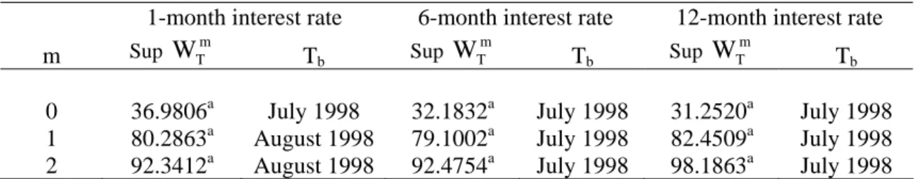
The Sup Wald test is performed on m = 0, 1 and 2 and the results are reported in Table 1. Significant break points are found in all the three interest rate series. The break point is identified as July 1998 for the 1-month interest rate for m = 0, and August 1998 for m = 1 and 2. For all the values of m, a significant break point is found at July 1998 for the other two interest rate series. The break points identified show that the interest rate went through a structural shift just before 1 September 1998 when the capital control measures were introduced.

Table 1: Sup Wald Statistics for Detection of Break Points in Interest Rate

1-month interest rate 6-month interest rate 12-month interest rate

m Sup WTm Tb Sup

m T

W _T_b Sup W_Tm _T_b

0 36.9806a July 1998 32.1832a July 1998 31.2520a July 1998

1 80.2863a August 1998 79.1002a July 1998 82.4509a July 1998

2 92.3412a August 1998 92.4754a July 1998 98.1863a July 1998

Notes: The 1% critical values are 13.02, 17.51 and 19.90, respectively, for an I(0) process. The corresponding critical values are 22.48, 30.36 and 38.35, respectively, for an I(1) process. See Vogelsang (1997, pp. 824-825).

(5)

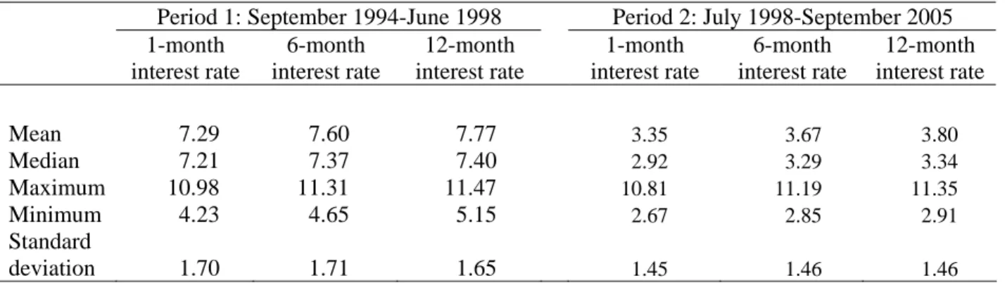
In the following analysis, we divide the period of study into two sub-periods. We use July 1998 as the starting point of the structural break. We therefore set the first sub-period to be from September 1994 to June 1998, and the second sub-period is from July 1998 to September 2005. The summary statistics in Table 2 show that the interest rates in the first period are relatively higher on average compared to the rates in the second period.

4. Time-series Properties

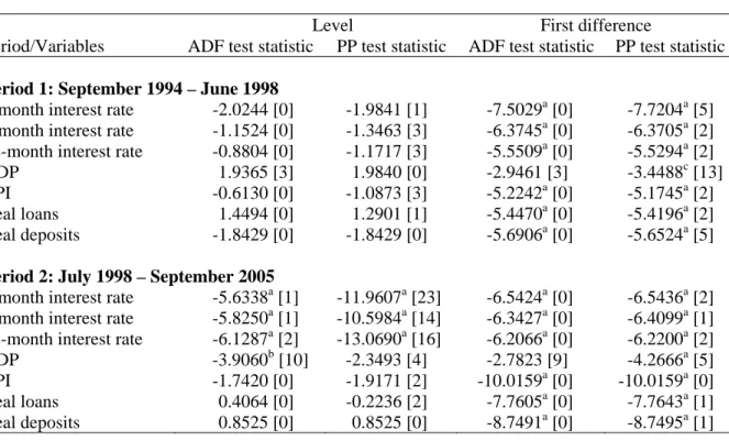
The augmented Dickey-Fuller and Phillips-Perron unit root tests are performed to examine the time-series properties of the series used in this study. The results in Table 3 indicate that the interest rate is integrated of order one in the first period, but the order of integration is zero in the second period. The results suggest that the stochastic trend in the interest rate found before implementation of capital controls no longer exists after the measures were put in place. This could have stemmed from the low interest-rate regime adopted by the authority in the second period. The other series used in the study (see below) include GDP, CPI, aggregate loans and deposits. All these series exhibited non-stationary behaviour in levels but stationarity is achieved after taking first difference.

Table 2: Summary Statistics for Interest Rate

Period 1: September 1994-June 1998 Period 2: July 1998-September 2005

1-month interest rate 6-month interest rate 12-month interest rate 1-month interest rate 6-month interest rate 12-month interest rate Mean 7.29 7.60 7.77 3.35 3.67 3.80 Median 7.21 7.37 7.40 2.92 3.29 3.34 Maximum 10.98 11.31 11.47 10.81 11.19 11.35 Minimum 4.23 4.65 5.15 2.67 2.85 2.91 Standard deviation 1.70 1.71 1.65 1.45 1.46 1.46

5. Responses of Bank Lending to Interest Rate Changes

The unit root test results show that we have a mixture of I(0) and I(1) processes. The autoregressive-distributed lag (ARDL) modelling with bounds testing approach (Pesaran and

Shin 1999, Pesaran et al. 2001) is adopted for further analysis. This testing procedure is

suitable for regressors that are of a mixture of I(0) and I(1) processes. Another advantage is that the approach is applicable even if the sample size is small.

The principle of the two-step procedure suggested by Cover (1992) and Dell’Ariccia and Garibaldi (1998) is adapted. The first step involves estimating a model that explains the

(6)

interest rate dynamics. As in these studies, the interest rate is postulated to be a function of GDP and CPI. The ARDL(p, q, r) model for the interest rate is

∆irt = µ + θ1irt-1 + θ2GDPt-1 + θ3CPIt-1 + ∑ α = p 1 i i ∆irt-i + ∑β = q 0 j j ∆GDPt-j + ∑ γ = r 0 k k ∆CPIt-k + εt (2)

and level variables are included as suggested by the modelling approach of Pesaran and Shin (1999) to account for possible cointegration among interest rate, GDP and CPI. Level relationship is present if the null hypothesis of H0: θ1 = θ2 = θ3 = 0 is rejected in equation (2).

This hypothesis is evaluated using the bounds F-test proposed by Pesaran et al. (2001). If the null hypothesis is not rejected, the level explanatory variables are dropped from the interest rate equation.

Table 3: Augmented Dickey Fuller (ADF) and Phillips-Perron (PP) Tests for Unit Roots

Level First difference

Period/Variables ADF test statistic PP test statistic ADF test statistic PP test statistic

Period 1: September 1994 – June 1998

1-month interest rate -2.0244 [0] -1.9841 [1] -7.5029a [0] -7.7204a [5]

GDP 1.9365 [3] 1.9840 [0] -2.9461 [3] -3.4488c [13]

CPI -0.6130 [0] -1.0873 [3] -5.2242a [0] -5.1745a [2]

Real loans 1.4494 [0] 1.2901 [1] -5.4470a [0] -5.4196a [2]

Real deposits -1.8429 [0] -1.8429 [0] -5.6906a [0] -5.6524a [5]

Period 2: July 1998 – September 2005

1-month interest rate -5.6338a [1] -11.9607a [23] -6.5424a [0] -6.5436a [2] 6-month interest rate -5.8250a [1] -10.5984a [14] -6.3427a [0] -6.4099a [1] 12-month interest rate -6.1287a [2] -13.0690a [16] -6.2066a [0] -6.2200a [2]

GDP -3.9060b [10] -2.3493 [4] -2.7823 [9] -4.2666a [5]

CPI -1.7420 [0] -1.9171 [2] -10.0159a [0] -10.0159a [0]

Real loans 0.4064 [0] -0.2236 [2] -7.7605a [0] -7.7643a [1]

Real deposits 0.8525 [0] 0.8525 [0] -8.7491a [0] -8.7495a [1]

Notes: The test regression contains a constant and time trend. Figures in brackets are lag lengths used in the test regression. The lag length is determined from the Schwarz information criterion for the ADF test and the Newey-West (1994) selection method using Bartlett kernel based estimators for the PP test.

a,b,c

Significant at 1%, 5% and 10%, respectively.

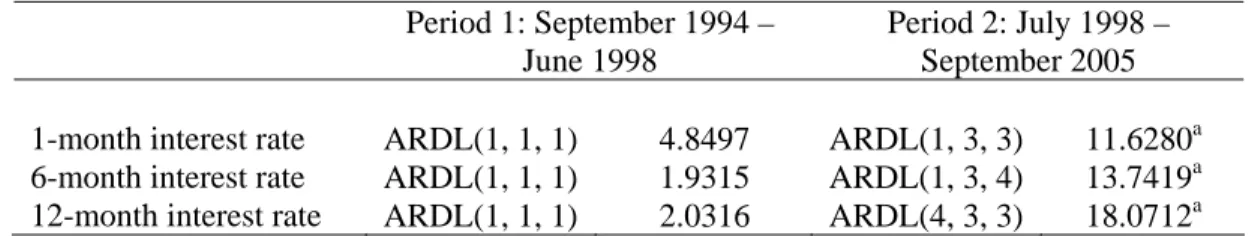
A search is conducted for p = q = r = 1,…, 6. A total of 216 equations are estimated for each interest rate series in each sub-period, and the Schwarz information criterion is used to select

(7)

the optimal lag order. The orders of ARDL are given in Table 4. For the selected model, the null hypothesis of no level relationship is rejected for all the three interest series in the second period. There is no evidence, however, to support the existence of level relationship for the first period. Therefore, lagged level variables are included only in the interest rate equations for the second period. Variables that are not significant are subsequently dropped from all the interest rate equations, and the final estimated models are reported in Appendix I.

The residuals of the estimated models (et) are used to generate the interest rate shocks as

equation (2) provides the baseline market expected interest rate. Any shocks in the money market are represented by the residual series of this equation. Following Dell’Ariccia and Garibaldi (1998), a positive shock to the money market interest rate is defined as:

tightt = max(et, 0) (3)

where else a negative shock is given by:

easyt = min(et, 0) (4)

Tight market conditions are the results of interest rate shocks from contractionary monetary policy while easy market conditions occur due to shocks from expansionary monetary policy.

Table 4: Bounds F-Test for Level Relationship among Interest Rate, GDP and CPI

Period 1: September 1994 – June 1998

Period 2: July 1998 – September 2005

1-month interest rate ARDL(1, 1, 1) 4.8497 ARDL(1, 3, 3) 11.6280a

Notes: The ARDL lag orders are selected using the Schwarz information criterion.

The 5% lower and upper limit of the critical bounds values are 3.79 and 4.85, respectively. The corresponding values at 1% are 5.15 and 6.36, respectively.

a

Significant at 1%.

The second stage of the two-step procedure involves estimating the loan equation. Total bank deposits are included in the model as they are important sources of funds for loan formation. The ARDL(p, q, r, s) model for the loan equation is specified as:

∆loant = µ + θ1loant-1 + θ2depositt-1 + ∑ α = p 1 i i ∆loant-i + ∑β = q 0 j j ∆depositt-j + ∑ γ = r 1 k k tightt-k +∑ λ = s 1 m m easyt-m + vt (5)

(8)

The contemporaneous terms of tightt and easyt are not included to allow for loans to react to

interest rate changes with a lag. The bounds F-test is used to test the null hypothesis of H0: θ1 = θ2 = 0 to examine if the level relationship between loan and deposit should enter

equation (5).

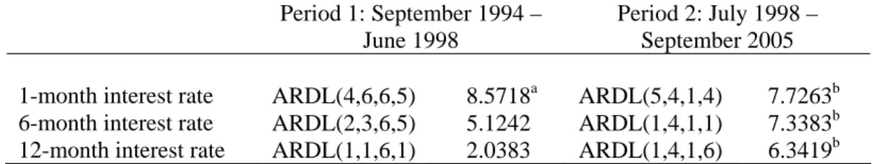
The lag orders for equation (5) are determined by searching through lag 1 to 6 for all of p, q, r and s. A total of 1,296 equations are estimated. The optimal lag orders based on the Schwarz information criterion consistently lead to selection of ARDL(1,1,1,1) in five out of six of the cases. These orders are low for analysis of the lag dynamics. We chose instead to tradeoff model parsimony and repeated the search using the Akaike information criterion. The lag orders of the final models are reported in Table 5. The bounds F-test provides evidence of level relationship between loans and deposits for the 1-month interest rate in the first period, and all the three interest rate series for the second period. The estimated loan equations are given in Appendix II.

Table 5: Bounds F-Test for Level Relationship between Real Loans and Real Deposits

Period 1: September 1994 – June 1998

Period 2: July 1998 – September 2005

1-month interest rate ARDL(4,6,6,5) 8.5718a ARDL(5,4,1,4) 7.7263b

6-month interest rate ARDL(2,3,6,5) 5.1242 ARDL(1,4,1,1) 7.3383b

12-month interest rate ARDL(1,1,6,1) 2.0383 ARDL(1,4,1,6) 6.3419b

Notes: The ARDL lag orders are selected using the Akaike information criterion.

The 5% lower and upper limit of the critical bounds values are 4.94 and 5.73, respectively. The corresponding values at 1% are 6.84 and 7.84, respectively.

a,b

Significant at 1% and 5%, respectively.

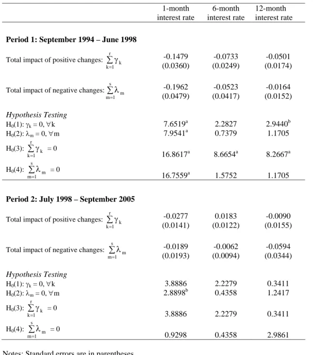
A series of four hypotheses are examined using the F- test on equation (5). These include the null hypotheses of H0(1): γk = 0, ∀k and H0(2): λm = 0, ∀m for examining if any of the

lagged interest rate shocks are significant. The null hypotheses of H0(3): ∑ γ

= r 1 k k = 0 and H0(4): ∑ λ = s 1 m m

= 0 are tested to evaluate the significance of the total impact of the positive and negative interest rate shocks, respectively.

The results in Table 6 indicate that positive interest rate shocks lead to reduction in bank lending in the first period. The rejection of H0(1) for the 1-month and 12-month interest rates

and H0(3) for all the interest rate series suggests that the tight interest rate policy is effective

in reducing credit availability in the loan market. There is, however, no evidence of significant credit expansion as a result of easy interest rate policy. On the contrary, negative shocks in the 1-month interest rate are found to lead to credit contraction.

(9)

Table 6: Impact of Interest Rate Changes on Real Loans

Total impact of positive changes: ∑ γ

= r 1 k k -0.1479 (0.0360) -0.0733 (0.0249) -0.0501 (0.0174)

Total impact of negative changes: ∑ λ

= s 1 m m -0.1962 (0.0479) -0.0523 (0.0417) -0.0164 (0.0152) Hypothesis Testing H0(1): γk = 0, ∀k 7.6519 a 2.2827 2.9440b H0(2): λm = 0, ∀m 7.9541 a 0.7379 1.1705 H0(3): ∑ γ = r 1 k k = 0 16.8617a 8.6654a 8.2667a H0(4): ∑ λ = s 1 m m = 0 16.7559a 1.5752 1.1705

Total impact of positive changes: ∑ γ

= r 1 k k -0.0277 (0.0141) 0.0183 (0.0122) -0.0090 (0.0155)

Total impact of negative changes: ∑ λ

= s 1 m m -0.0189 (0.0193) -0.0062 (0.0094) -0.0594 (0.0344) Hypothesis Testing H0(1): γk = 0, ∀k 3.8886 2.2279 0.3411 H0(2): λm = 0, ∀m 2.8898 b 0.4358 1.2417 H0(3): ∑ γ = r 1 k k = 0 3.8886 2.2279 0.3411 H0(4): ∑ λ = s 1 m m = 0 0.9298 0.4358 2.9861 Notes: Standard errors are in parentheses.

The F-statistics are reported for hypothesis testing. a,b

Significant at 1% and 5% respectively.

In the second period, the results of the hypothesis testing show that bank lending does not respond to tight interest rate policy. The total impact of positive interest rate shocks in all cases is not significant. There is a marked difference in the results when compared to those of the first period.

(10)

Again, there is some evidence of credit contraction following negative shocks in the 1-month interest rate. Expansionary monetary policy through the bank lending channel has not been effective. According to the interpretation of Tee and Goh (2006), the commercial banks are prudent in their lending in easy money market conditions when interest rates are generally low. Such behaviour could be because when the rates are low, the risk of lending becomes higher and the profit margin is tighter.

4. Conclusion

This paper shows that the interest rates in the money market of Malaysia went through a significant structural shift on the eve of the imposition of capital controls by the government. The shift characterises a period of relatively high-interest-rate regime (first period), and another regime of low interest rates (second period). The desirable outcome of bank lending contraction following positive interest rate shocks occurred only in the first period but not in the second period. The results provide evidence that the effectiveness of bank lending channel as a transmission mechanism for the conduct of monetary policy differs according to the interest rate regime.

References

Bank Negara Malaysia.(various issues) Monthly Statistical Bulletin, Bank Negara Malaysia:

Kuala Lumpur.

Bernanke, B. and A. Blinder (1992) The Federal funds rate and the channels of monetary

transmission, American Economic Review, 82, 901-921.

Bernanke, B. and M. Gertler (1995) “Inside the Black Box: The Credit Channel of Monetary

Policy Transmission” Journal of Economic Perspectives9, 27-48.

Bernanke, Ben S. (1993) “How Important is the Credit Channel in the Transmission of

Monetary Policy?: A Comment” Carnegie-Rochester Conference Series on Public

Policy 39, 47-52.

Bondt, Gabe de (2000) Financial Sturcture and Monetary Transmission in Europe, Edward

Elgar: Cheltenham.

Chong, C.S. and K.L. Goh (2005) “Intertemporal Linkages of Economic Activity, Stock

Price and Monetary Policy in Malaysia,” Asia Pacific Journal of Economics and

Business9, 48-61.

Cover, J. P. (1992) “Asymmetric Effects of Positive and Negative Money-supply Shocks” Quarterly Journal of Economics CVII, 1261-1282.

Dell’Ariccia, G. and P.Garibaldi (1998) Bank lending and interest rate changes in the

dynamic matching model, IMF Working Paper, No.WP/98/93.

Doraisami, A. (2004) “From Crisis to Recovery: The Motivations for and Effects of

(11)

Garretsen, H. and J. Swank (1998) “The Transmission of Interest Rate Changes and the Role

of Bank Balance Sheets: A VAR-Analysis for the Netherlands,” Journal of

Macroeconomics20, 325-339.

Garretsen, H. and J. Swank (2003) “The Bank Lending Channel in the Netherlands: The

Impact of Monetary Policy on Households and Firms,” De Economist, 151, 35-51.

Goldstein, M. and M.S. Khan (1976) “Large versus Small Price Changes and the Demand for

Imports” IMF Staff Papers23, 200-225.

Hernando, I. and J. Martinez-Pages (2001) “Is There a Bank Lending Channel of Monetary Policy in Spain?” Working Paper Series No. 99, European Central Bank.

Hubbard, R.G. (1994) “Is there a ‘Credit Channel’ for Monetary Policy?” NBER Working Paper no. 4977, Cambridge, Massachusetts.

Hulsewig, O., P. Winker and A. Worms (2001) “Bank Lending in the Transmission of Monetary Policy: A VECM Analysis for Germany,” Working Paper 08/2001, School of Busines Administration, International University in Germany.

Kakes, J. and J.E. Sturm (2001) “Monetary Policy and Bank Lending: Evidence from German Banking Groups,” mimeo, De Nederlandsche Bank/University of Groningen. Kakes, J. (2000) “Identifying the Mechanism: Is There a Bank Lending Channel of Monetary

Transmission in the Netherlands?” Applied Economics Letters7, 63-67.

Kashyap, A.K. and J.C. Stein (1997) “The Role of Banks in Monetary Policy: A Survey with

Implications for the European Monetary Union” Federal Reserve Bank of Chicago

Economic Perspectives21, 2-18.

Kaufmann, S. and M.T. Valderrama (2004) “The Role of Bank Lending in Market-Based and

Bank-Based Financial Systems” Monetary Policy & the Economy2, 88-97.

Morris, C.S. and G.H. Sellon, Jr. (1995) “Bank lending and Monetary Policy: Evidence on a

Credit Channel”, Federal Reserve Bank of Kansas City Economic Review, Second

Quarter, 59-75.

Pesaran, M.H. and Y. Shin (1999) “An Autoregressive Distributed Lag Modelling Approach

to Cointegration Analysis” in: Econometrics and Economic Theory in the 20th

Century: The Ragnar Frisch Centennial Symposium by S. Strom, Ed., Cambridge: Cambridge University Press.

Pesaran, M.H., Y. Shin, and R.J. Smith (2001) “Bounds Testing Approaches to the analysis

of Level Relationships” Journal of Applied Econometrics16, 289-326.

Tee, C.G. and K.L. Goh (2006) “Impacts of Unanticipated Interest Rate Shocks on

Commercial Bank Lending in Malaysia” in Statistics In Action by S. Nagaraj, K.L.

Goh and N.P. Tey, Eds., Kuala Lumpur: University of Malaya Press.

Vogelsang, T.J. (1997) “Wald-type Tests for Detecting Breaks in the Trend Function of a

(12)

APPENDIX I

The Estimated Interest Rate Equations

1-month Interest rate 6-month Interest rate 12-month Interest rate

constant 0.1979a (0.0645) 0.1986a (0.0506) 0.2015a (0.0479)

∆GDPt-1 -13.2189b (6.4182) -14.2024a (5.0361) -16.5937a (4.7662)

constant 0.3966a (0.0734) 0.4119a (0.0694) 0.4731a (0.0682) irt-1 -0.1276 a (0.0205) -0.1151a (0.0170) -0.1305a (0.0164) ∆irt-1 0.2753a (0.0793) 0.2645a (0.0736) 0.2676a (0.0688) ∆irt-4 -0.2554 a (0.0674) ∆GDPt -12.7118 a (4.1785) -16.1426a (4.3181) -20.1493a (4.2827) ∆GDPt-1 10.1958 b (4.9883) 9.9610b (4.6906) ∆GDPt-2 16.2213a (5.4122) 12.9231a (4.8677) 13.8435a (4.5719) ∆GDPt-3 -14.8262a (4.7329) -16.7734a (4.1655) -16.1143a (3.9208) ∆CPIt-1 30.0033 a (11.1674) 34.1587a (9.8425) 33.6462a (9.2360) ∆CPIt-2 25.0337 b (12.0029) ∆CPIt-3 -41.0870 a (12.0336) -39.7682a (10.2940) -39.7597a (9.6161)

Notes: Standard errors are in parentheses. a,b

(13)

APPENDIX II

The Estimated Loans Equations

constant -0.2014 (0.5810) 0.0179c (0.0096) 0.0149b (0.0054) loant-1 -0.7094b (0.2879) depositt-1 0.7265 b (0.3291) ∆loant-1 0.1822 (0.2672) 0.0417 (0.2167) 0.1085 (0.1882) ∆loant-2 0.0782 (0.3436) -0.2863 (0.2862) ∆loant-3 0.4457c (0.2456) ∆loant-4 0.2136 (0.2479) ∆depositt -0.1041 (0.1508) 0.0395 (0.1232) 0.0414 (0.1029) ∆depositt-1 -0.8658 b (0.2878) -0.0141 (0.1347) 0.0581 (0.1066) ∆depositt-2 -0.4988 c (0.2363) 0.1127 (0.1231) ∆depositt-3 -0.4377b (0.1889) 0.0613 (0.1184) ∆depositt-4 -0.3984b (0.1625) ∆depositt-5 -0.3169 c (0.1710) ∆depositt-6 -0.2384 c (0.1291) tightt-1 0.0010 (0.0094) -0.0165 (0.0147) 0.0030 (0.0108) tightt-2 0.0144 (0.0123) 0.0143 (0.0140) 0.0089 (0.0098) tightt-3 -0.0112 (0.0122) -0.0063 (0.0150) -0.0177c (0.0095) tightt-4 -0.0617a (0.0108) -0.0255c (0.0122) -0.0281b (0.0102) tightt-5 -0.0440 c (0.0208) -0.0227 (0.0186) -0.0074 (0.0116) tightt-6 -0.0464 c (0.0226) -0.0166 (0.0145) -0.0089 (0.0088) easyt-1 -0.0210 c (0.0100) 0.0109 (0.0245) -0.0164 (0.0152) easyt-2 -0.0362 a (0.0115) -0.0079 (0.0164) easyt-3 -0.0671 a (0.0132) -0.0244 (0.0180) easyt-4 -0.0354 c (0.0178) -0.0112 (0.0188) easyt-5 -0.0365c (0.0182) -0.0197 (0.0179)

(14)

Appendix II (cont’d)

constant -0.0920 (0.1908) 0.0033 (0.1702) 0.0795 (0.1731) loant-1 -0.1257 a (0.0447) -0.1230a (0.0397) -0.1643a (0.0530) depositt-1 0.1318 a (0.0369) 0.1213a (0.0330) 0.1558a (0.0454) ∆loant-1 0.2377 b (0.1052) 0.2403b (0.1037) 0.2276b (0.1034) ∆loant-2 -0.1282 (0.1048) ∆loant-3 0.0332 (0.1119) ∆loant-4 0.1799 (0.1309) ∆loant-5 -0.2508 b (0.1241) ∆depositt 0.6603 a (0.1006) 0.5986 (0.1002) 0.6063 (0.1056) ∆depositt-1 -0.2079 (0.1248) -0.0702 (0.1208) -0.1235 (0.1235) ∆depositt-2 0.0045 (0.1191) -0.0563 (0.1054) -0.1047 (0.1082) ∆depositt-3 0.0715 (0.1262) 0.0386 (0.1097) 0.0306 (0.1134) ∆depositt-4 -0.3765 a (0.1181) -0.3377a (0.1150) -0.3393a (0.1183) tightt-1 -0.0278 c (0.0141) 0.0183 (0.0122) -0.0090 (0.0155) easyt-1 0.0163 (0.0121) -0.0062 (0.0094) 0.0015 (0.0118) easyt-2 -0.0093 (0.0070) -0.0084 (0.0112) easyt-3 -0.0047 (0.0071) -0.0209c (0.0115) easyt-4 -0.0209a (0.0072) -0.0230b (0.0106) easyt-5 -0.0066 (0.0101) easyt-6 -0.0020 (0.0102)

Notes: Standard errors are in parentheses. a,b,c