Hedging speculation, and investment in balance-sheet triggered currency crises

Darmstadt Discussion Papers

in Economics

Hedging, Speculation, and Investment in Balance-Sheet Triggered

Currency Crises

Andreas Röthig, Willi Semmler and Peter Flaschel

Nr. 168

Arbeitspapiere

des Instituts für Volkswirtschaftslehre

Technische Universität Darmstadt

ISSN: 1438-2733

E

Hedging, Speculation, and Investment

in Balance-Sheet Triggered Currency Crises

Andreas R¨othig

_{, Willi Semmler}

_{and Peter Flaschel}

February 2006

Abstract

This paper explores the linkage between corporate risk management strategies, investment, and economic stability in an open economy with a flexible exchange rate regime. Firms use currency futures contracts to manage their exchange rate exposure – caused by balance sheet effects as in Krugman (2000) – and therefore their investments’ sensitivity to currency risk. We find that, depending on whether futures contracts are used for risk reduction (i.e., hedging) or risk taking (i.e., specula-tion), the implied magnitudes of recessions and booms are decreased or increased. Corporate risk management can therefore substantially affect economic stability on the macrolevel.

Keywords: Mundell-Fleming-Tobin model, foreign-debt financed investment,

cur-rency crises, real crises, curcur-rency futures, hedging, speculation.

JEL Classification: E32, E44, F31, F41.

∗_{We would like to thank Ingo Barens for extensive discussions. We are also grateful to}

partici-pants of the ‘Colloquium of Quantitative Economics, Statistics and Econometrics’ at the University of Bielefeld.

∗∗_{Institute of Economics, Darmstadt University of Technology, and Center for Empirical}

Macroe-conomics, University of Bielefeld.

†_{Center for Empirical Macroeconomics, University of Bielefeld, and New School University, New}

York.

1

Introduction

In this paper we investigate the implications of corporate risk management in a balance sheet-triggered currency crises model as it was introduced in the literature

by Krugman (1999, 2000). First, we investigate the real-financial interface on the microeconomic level. Firms’ investment policies are assumed to depend on foreign currency denominated debt. The value of this debt (measured in domestic currency)

is thus subject to exchange rate fluctuations. The higher the debt burden measured in domestic currency, the less the firms can invest, due to the operation of credit constraints. Second, we explore the relevance of these microeconomic factors for

macroeconomic stability in a flexible exchange rate regime. A currency crisis (i.e. a steep devaluation of the domestic currency) will increase firms’ debt burden and, therefore, have a deleterious effect on investment due to its financing conditions.

Significantly decreasing investment leads in turn to large output losses, as described by the IS equilibrium relationship or a dynamic multiplier process.

Hence, we have a feedback chain leading from large devaluations via the

foreign-debt burden of firms and their investment possibilities to macroeconomic activity and employment. In this basic situation, we give in this paper – compared to Flaschel and Semmler (2006) – the firms an instrument to interrupt the feedback channel right

at the beginning. We assume that firms can trade currency futures to influence their investment’s exposure to currency risk. In the literature, widespread corporate use of derivative securities is well documented. DeMarzo and Duffie (1995, p. 743-744)

point out that the demand for risk management vehicles by corporations was an important component of the “explosion in financial innovation” that has occurred

in the 1980s and 1990s. There are a number of reasons for firms to implement such hedging strategies.1_{However, firms have also incentives to speculate.}2 _Risk

management, in our approach, therefore comprises strategies for risk reduction as

well as strategies for risk taking.

There are several articles investigating the link between demand for financial deriva-tives by corporations and firms’ investment policies.3_{However, there is rarely any}

lit-erature dealing with the implications of the ‘financing-risk management-investment’ interface for macroeconomic behavior. This paper therefore examines the impact of risk management strategies on aggregate investment and on aggregate demand

and output. We show that the magnitude of potential recessions and booms signif-icantly depends on whether corporations use financial derivatives for hedging or for speculation.

The paper is organized as follows. Section 2 presents a Flaschel and Semmler (2006) type Mundell-Fleming-Tobin (MFT) model adjusted to allow for the treatment of Krugman (2000) type currency crises situations. Section 3 introduces linear hedging

and speculation into the model and considers their implications. Section 4 presents simulation results implied by our modification of the MFT approach to

macroeco-1_{See e.g. Stulz (1984), Smith and Stulz (1985), Fung and Leung (1991), Froot, Scharfstein and} Stein (1993), Nance, Smith and Smithson (1993), Beatty (1999), and Albuquerque (2003).

2_{See e.g. Guay (1999).}

3_{See e.g. Froot, Scharfstein and Stein (1993, 1994), Tufano (1998), Gay and Nam (1998), Fatemi} and Luft (2002), and Lin and Smith (2005).

nomics. In addition to hedging and speculation, the role of futures trading costs and the impact of capital flights is also investigated. Finally, Section 5 concludes.

2

The basic Krugman version of the MFT model

port-folio approach “which owes much to Tobin”4_{. The model consists of a goods market}

equilibrium curve (an IS curve) and the a financial markets equilibrium curve (called AA curve). We characterize equilibrium in the goods market by the condition that

production Y must be equal to aggregate demand, i.e., to the sum of consumption

C, investment I, government expenditure G, and net exports NX:5

Y =C(Y −δK¯ −T¯) +I(e) + ¯G+NX(Y,Y¯∗_{, e) (1)}

Consumption and government expenditures are defined as customary in an IS rela-tionship. The representation of investment and net exports needs some explanation. As usual, net exports depend negatively on domestic output Y and positively on

foreign output ¯Y∗_{. The main feature of the model is therefore the interface between}

the responses of investment (here assumed to depend negatively on the exchange rate as in Krugman (2000)) and net exports to exchange rate changes. A

depreci-4_{Rødseth (2000, p. 169) with a modified investment behavior of firms as introduced in Krugman} (2000).

5_{This equation can be reduced to an equation representing the domestic goods market solely} if the domestic absorption of foreign goods is cancelled against the import component in the net export function.

ation of the domestic currency which is equivalent of a rise in the price of foreign exchange will make domestic goods more competitive. Ceteris paribus, net exports

will increase (NXe > 0) if the Marshall-Lerner conditions are assumed to hold. If

this is the only effect on the goods market, the IS curve will be upward sloping in the output – exchange rate phase space. Yet investment is here assumed to depend

on the exchange rate as well.

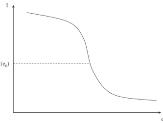
Krugman (2000) introduces an investment function where firms have substantial debts denominated in foreign currency. A depreciation of the domestic currency

will increase their debt, measured in domestic currency, and therefore worsen the balance sheets of these firms. These balance sheet problems will lead the firms – voluntarily or unvoluntarily – to cut back investment (Ie <0). Figure 1 shows this

type of an investment function. The function is downward sloping and due to credit rationing and supply side bottelnecks on both sides nonlinear. The nonlinearity is due to the fact that exchange rate changes affect investment strongly only at

intermediate values ofe, around steady state investment I(e0). The reason is that,

for very high or very low values of e, changes of the exchange rate do no longer have such a strong impact effects on investment. In the case of high values of e,

for example, the debt value measured in domestic currency is already very large and the resulting investment is already close to its minimal sustainable value. In this situation smaller exchange rate changes will not have the same impact as for

intermediate ranges around I(e0). At low exchange rates investment plans can be

I

I(e₀)

e

Figure 1: The Krugman type investment function.

The nonlinearity of the investment function allows for the possibility of a

balance-sheet driven financial as well as real crisis. At mid-range-values ofewhere investment reacts strongly to exchange rate changes, these negative balance sheet effects may outweigh the positive competitiveness effects (Ie > N Xe). This will cause the goods

market curve to bend backward for such exchange rate changes. In the case of extraordinarily high or low values of e, where investment is not that sensitive to changes in the exchange rate, the competitiveness effects however outweighs the

balance sheet effects (NXe > Ie). In this case the goods market curve is upward

sloping. Using the Implicit Function Theorem, we can derive the slope of the IS curve analytically:

Y0_{(e) =−} Ie+NXe

CY +NXY −1

(2)

negative. Hence,Yeis upward sloping ifNXe> Ieand backward bending otherwise.

The financial sector in this model is represented by the financial markets equilibrium

curve (AA curve). The AA relation consists of the following equations:6

Risk premium (definition): ξ=r−r¯∗ _{−ε (3)}

Expected rate of depreciation: ε=βε(e_e0 −1), εe ≤0 (4)

Private Wealth: Wp =M0+B0 +eFp0 (5)

LM-Curve: M = m(Y, r), mY >0, mr <0 (6)

Demand for foreign bonds: eFp =g(ξ, Wp), gξ <0, gWp ∈(0,1) (7)

Demand for domestic bonds: B = Wp −m(Y, r)−g(ξ, Wp) (8)

Foreign exchange market: F¯∗ _=F

p+Fc (9)

Equation (3) defines the risk premium ξ as the difference between domestic and

foreign rates of return on bonds, i.e., by the difference between the domestic interest rate and the foreign one, the latter augmented by the expected rate of currency depreciation. Equation (4) defines the expected rate of currency depreciation,

mak-ing use of a standard regressive expectations mechanism as it is extensively used in Rødseth (2000), with εe ≤ 0 and ε(e0) = 0 for the steady state exchange rate level

e0. Economic agents have perfect knowledge of the future equilibrium exchange rate

and therefore expect the actual exchange rate to adjust to the steady state value after the occurrence of a shock. Flaschel and Semmler (2006) describe these

pectations, allowing agents to behave forward looking, as asymptotically rational. This assumption ensures that obtained instability is not caused by the expectations

formation process, but due to other forces in the model of this paper. Equation (5) defines initial private sector wealth as a portfolio of domestic money M0, domestic

bonds B0, and foreign bond holdings eFp0. Equations (6), (7), and (8) present the

three asset demand equations of the private sector. Equation (9) is the equilibrium condition for the foreign exchange market where the total amount of foreign bonds held in the domestic economy ¯F∗ _{equals domestic private foreign bond holdings eF}

p

plus the central bank’s foreign bond holdings Fc. We assume as in Rødseth (2000)

that domestic bonds cannot be traded internationally which implies that the for-eign bond holding in the domestic economy is only changed (sluggishly) through

imbalances in the current account (and not by international capital movements). Inserting equation (3) and equation (5) in equation (7) gives the financial markets equilibrium curve (AA curve):

eFp =g(r(Y, M0)−r¯∗−βε(

e0

e −1), M0+B0+eFp0) (10)

Note that in a flexible exchange rate regime the central bank need not intervene on the foreign exchange market, i.e., Fp can be considered a given magnitude in such a

case. The slope of the AA curve is determined by the Implicit Function Theorem:

e0_{(Y) =−} gξ∗rY

−gξ∗εe+ (gWp−1)∗Fp0

<0 (11)

Fp0 ≥0. In the following sections we will assume the AA curve to be linear to ease graphical expositions. e IS e₁ Y₁ E1 AA Y₂ Y₃ e2 e₃ E₃ E₂ Y

Figure 2: The IS-AA model.

Figure 2 shows the IS-AA model with multiple equilibria. Such a situation occurs if the elasticity of substitution between domestic and foreign bonds (to be measured

by the first partial derivative of the g−function) is assumed to be sufficiently high. There are then two equilibria on the upward sloping segments of the IS curve (E1

andE3) and one equilibrium on the backward bending segment of the IS curve (E2).

In equilibrium E1 and E3 the competitiveness effect dominates the balance sheet

effects (NXe > Ie), whereas in equilibrium E2 the balance sheet effect dominates

the competitiveness effect (Ie > NXe).

J =     βY[CY +NXY −1] βY[Ie+NXe] βe[gξ∗rY] βe[−gξ∗εe+ (gWp −1)∗Fp0]    

Consideringgξ<0, rY >0, gWp ∈[0,1] andεe≤0, we obtain the following signs:

J =     − ? − −    

The stability of the equilibria (E1, E2, E3) depends on the sign of ‘?’ in the Jacobian

and therefore on the question which effect (NXe or Ie) dominates the other one.

As we already mentioned, in equilibrium E1 and E3 the IS curve is upward sloping

and NXe > Ie holds. In this case the ‘?’ has a positive sign. The determinant of

the Jacobian is positive (det(J(E1,3))>0) and the trace is negative (tr(J(E1,3))<0).

Equilibrium E1 and E3 are stable. Yet, equilibrium E2 is unstable since Ie > NXe

which results in a negative sign of ‘?’. With a negative ‘?’, the determinant7 _and

the trace of the Jacobian are both negative (det(J(E1,3))<0 and tr(J(E1,3))<0).8

The three equilibria presented in Figure 2 represent three different states of the economy. EquilibriumE1 stands for the stable ‘good equilibrium’ with high output

and a low exchange rate. E2 represents the fragile intermediate equilibrium,9 and

E3 is the stable ‘crisis equilibrium’ with low output and a high exchange rate. 7_{Since the slope of the IS-curve is less negative than the slope of the AA-curve.}

8_{For more details on such a stability analysis see the ‘trace-determinant plane’ in Hirsch, Smale} and Devaney (2004, p. 63).

3

Introducing linear hedging and speculation

depreciation of the domestic currency) will increase the value of foreign currency de-nominated debt in terms of the domestic currency. If the debt has to be settled, or if specific debt payments occur after the devaluation, the firm incurs a loss. Moreover

their balance sheet and the implied net worth of firms may be considered as measure of the credit-worthiness of firms and lead to credit rationing in cases where large depreciations occur. By contrast, in the case of an appreciation of the domestic

cur-rency, the value of the debt of firms is reduced and their credit worthiness increased. Figure 3 illustrates the value of a single payment depending on the exchange rate.

Payoff

e0

Profit

e Loss

Figure 3: Firm’s payoff depending on e.

Assume now that the firms have the possibility to enter into futures contracts in

more risk (speculation). In our model, futures trading activity affects the investment function which has to be reformulated then as a function I(e, fd_):

I(e, fd_{) = I(e}

0)−(ArcT an(e)−fd∗ArcT an(e))−cf ∗fd (12)

with demand for futures contracts given by fd_{, and the costs associated with such}

futures trading given by cf. We assume that futures demand fd equals futures

supply fs_:

fd=fs =f (13)

If we only allow for hedging activities we get 0≤fd _{≤1. In the case f}d _{= 0 there}

is no demand for futures and therefore no hedging activity. In this case, we get the

following investment function10

I(e, fd_{) =I(e}

0)−ArcT an(e) (14)

which corresponds to the graphical representation of the Krugman (2000) investment function presented in Figure 1.

If fd _{= 1 we speak of a perfect hedge since negative effects of e on investment are}

completely offset by positive effects ofe on the futures position (i.e., (ArcT an(e)−

fd_{∗ArcT an(e)) = 0 in equation (12)). Hence, investment is not exposed to currency}

risk anymore. Investment stays on its steady state level I(e0) minus the hedging

costs cf:

I(e, fd_{) = I(e}

0)−cf (15)

For values of fd _{between 0 and 1, the futures position partly offsets investment’s}

exposure to currency risk.

Payoff e0 Spot Position Long Futures Position Hedged Position Profit Loss e

Figure 4: Firm’s perfectly hedged payoff.

Figure 4 illustrates a perfect hedge for a specific spot payment. The futures position generates profits if the spot position generates losses due to exchange rate changes.

Profits and losses sum up to zero. It is important to note that with this linear hedging strategy it is not possible to benefit from an appreciation. If the spot position generates profits, the futures position will generate losses, again summing

up to zero. If all single payments of firms are hedged this way, the investment function is independent of exchange rate movements.

Summarizing, we have the following representation of the investment function in the

I(e, fd_{) =}               

I(e0) = ¯I if f irms are perf ectly hedged (fd= 1).

I(e, fd_{) if f irms do not hedge perf ectly (0< f}d_<1).

I(e) if f irms do not hedge at all (fd_{= 0).}

(16)

In order to analyze speculation we have to allow for negative values offd_{. If we set,}

for example,fd_{=−0.5, we get}

I(e, fd_{) = I(e}

0)−(ArcT an(e)−(−0.5)∗ArcT an(e))−cf∗|−0.5| ⇒I(e0)−cf (17)

⇒I(e0)−1.5∗ArcT an(e)−0.5∗cf (18)

Note that we have multiplied the absolute value of fd _{with the trading costs c} f

in order to guarantee that the costs affect investment negatively. Firms take on risk in the futures markets and, therefore, increase the sensitivity of investment

to exchange rate changes. Figure 5 presents this risk-taking strategy connected to a specific payment. Speculation affects the slope of the curve leading to higher sensitivity of the cash flow.

Payoff e e0 Spot Position Speculative Position Profit Loss

Figure 5: Firm’s payoff plus speculation.

4

Simulation studies of the model

In this section we simulate the model in order to get more insights into the mecha-nisms that determine the model’s outcomes. We will concentrate on the interaction

between investment and net exports, and therefore on the slope of the IS curve. We here define the investment function by

I(e) =I(e0)−b1∗(ArcT an(b2∗e)−fd∗ArcT an(b2∗e))−cf ∗ |fd| (19)

We set I(e0) = 0, b1 = 100, and b2 = 0.1.11Figure 6 shows the investment function

with fd _{= 0. The ArcTan investment function is a good representation of the}

Krugman(2000) function as presented in Figure 1.

11_{Note that, the parameters are not chosen in accordance with empirical data, but in order to} fit the graphical representation.

Figure 6: ArcTan investment function.

Next, we introduce this investment function into the IS curve of the model:

a1∗e3+I(e0)−b1∗(ArcT an(b2∗e)−fd∗ArcT an(b2∗e))−cf∗ |fd| −Y = 0 (20)

witha1∗e3 representing net exports.12 Again, we focus on the interaction of output

Y and the exchange rate e. All other variables and relations like consumption C

and government expenditure ¯G are set to zero for reasons of simplicity. We set

a1 = 0.0001 and get the following IS relation:

0.0001∗e3_{−100∗(ArcT an(0.1∗e)−f}d_{∗ArcT an(0.1∗e))−c}

f∗ |fd| −Y = 0 (21)

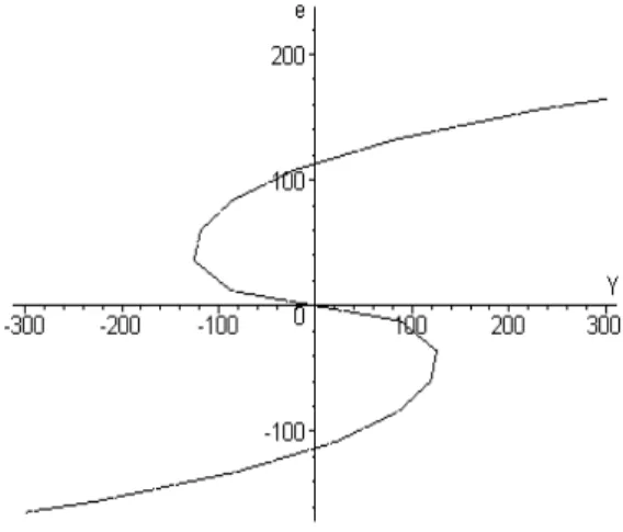
Figure 7: IS Curve.

Figure 7 shows the IS curve without futures trading (fd_{= 0). In the mid-range of}

e, where e goes from about −50 to 50, the IS curve bends backward. In the next sections we will model the hedging activity and also speculation as well as the role of futures trading costs.

4.1

Hedging activity

In this section we investigate the impact of corporate hedging on economic stability.

In the context of our model, we allow fd _{to range from 0 to 1. Moreover, we set}

Figure 8: Investment function with fd _{= 0, f}d _{= 0.5, and f}d_{= 1.}

Figure 9: IS Curve with fd _{= 0 (solid line), f}d _{= 0.5 (dotted line), and f}d _{= 1}

(dashed line).

Figures 8 presents the investment function for different hedging-levels (fd _{= 0,}

fd _{= 0.5, and f}d _{= 1). Figure 9 illustrates the effect of these various hedged}

investment functions on the IS relation. The investment function linearizes with growing hedging activity which in turn reduces the backward bending segment of

the IS curve. Figure 10 shows the effects of growing hedging activity on the IS curve with fd _{ranging from 0 to 1.}

Figure 10: IS curve with fd _{ranging from 0 to 1.}

Although the investment function is linear in the case of perfect hedging (fd _{= 1),}

the IS curve is still nonlinear. This is due to our definition of net exports. However, in the case of a perfectly hedged investment function, the IS curve slopes strictly up-wards. There is no backward bending segment and therefore, there are no multiple

equilibria. To make this point more obvious, we introduce a very simple represen-tation of the AA curve into the model. Again, we focus on the ‘Y-e interface’ and ignore all other influences. As we assume the AA curve to be linear and downward

sloping, we define the AA curve simply as e+Y = 0.

Figure 11 shows the IS-AA model with fd _{= 0, f}d _{= 0.5, and f}d _{= 1. In the}

case without hedging (fd _{= 0) we have three equilibria. Equilibrium A represents}

the ‘good equilibrium’, B is the intermediate steady state equilibrium, and C is the ‘crisis equilibrium’. If half of the investment is hedged (fd _{= 0.5), there are still}

reduced. This is because spot losses and futures profits (or spot profits and futures losses respectively) are more and more balanced with growing hedging activity. If

investment is perfectly hedged (fd_{= 1) only the intermediate equilibrium B remains.}

Moreover, this formerly fragile equilibrium is now stable since NXe+Ie ≥ 0 (i.e.

the IS curve does not bend backward).

Figure 11: IS-AA model with fd _{= 0 (solid line), f}d _{= 0.5 (dotted line), and}

fd_{= 1 (dashed line).}

Figure 12 presents the IS-AA model forfd_{ranging from 0 to 1. Note that, forf}d_{= 1}

there is only one equilibrium determined by the intersection of the AA-plane with

the IS curve. With fd _{going from 1 to 0, the backward bending segment of the IS}

Figure 12: IS-AA model from different viewpoints.

4.2

Speculation

In this section, futures demand fd _{is in the range [−1,0], where f}d _{= 0, again, is}

the case without futures trading and therefore without speculation. If fd _{= −1,}

firms double their exposure to currency risk. Of course, speculation in general is not bound to doubling the existing risk. However, analyzing futures trading for values

fd _{<−1 does not yield additional insights. Therefore, we restrict our investigation}

to the range−1≤fd _≤0.

Figures 13 and 14 show the impact of speculation on the IS-AA model. In contrast

to the case where firms hedge, here, the backward bending segment of the IS curve increases. This leads to the possibility of more severe recessions but also to the possibility of larger economic booms. Note that, again, we set futures trading costs

Figure 13: IS-AA model with fd _{= 0 (solid line), f}d _{= −0.5 (dotted line), and}

fd_{=−1 (dashed line).}

Figure 14: IS-AA model with speculation from different viewpoints.

4.3

Futures trading costs

Thus far we have set futures trading costs to zero. In this section we discuss the role of futures prices in the case where firms use futures to hedge their currency

price at all.”13 _{In general, traders have to deposit an initial margin at the exchange}

when a position is opened or increased. If a futures position generates losses, the

holder of the position has to deposit an additional amount reflecting his losses. However, if the futures position generates profits, the holder of the futures position obtains payments. Nevertheless, we tread these initial margin requirements as costs

since they reduce the firms’ financial means to invest. Additionally, cf contains

other costs associated with futures trading, including costs of information, costs of training the financial staff, and costs of implementing sophisticated risk assessment

procedures.

Figure 15: Perfectly hedged economy with hedging costs cf = 0, cf = 50, and

cf = 100.

Figure 15 presents the perfectly hedged economy for different values ofcf. Increasing

costs have a negative effect on investment leading to reduced output. Figure 16 compares the IS curve without hedging to a perfectly hedged IS curve withcf = 200.

For this high value of cf, the perfectly hedged equilibrium is inferior to the crisis

equilibrium in the case without hedging.

Figure 16: Perfect hedge (fd_{= 1) and ‘no hedge’ (f}d _{= 0) with c}

f = 200.

However, the values of cf in Figures 15 and 16 were chosen arbitrarily in order to

stress the linkage between trading costs and output. The extremely high value in

Figure 16 does not correspond to empirical findings. Generally, trading financial derivatives on organized exchanges costs only a fraction of contract size. Trading over-the-counter derivatives, often, does not involve any trading costs. Therefore,

in reality, futures trading costs will not have such an direct impact on output. Nevertheless, there is an indirect linkage since firms base their risk management decision, and hence, their exposure to specific risks at least partly on the costs of

risk management. In this way, trading costs have an impact on the risk exposure of investment and therefore on output.

4.4

Private asset allocation and capital flight

In the previous sections we investigated the role of firms’ risk management and investment strategies on economic stability. We therefore focussed on the goods

market equilibrium curve. We assumed that firms can manage their exposure to currency risk and hence influence their investments’ sensitivity to exchange rate changes.

Here we now pay attention to the risk of private asset holders. We introduce a new parameterα into the financial markets equilibrium curve which represents this risk of private asset holders:14

eFp =g(r(Y, M0)−r¯∗−βε(

e0

e −1), M0+B0+eFp0, α) (22)

If there is a depreciation of the domestic currency (i.e., e increases) the value of foreign bonds demand eFd

p measured in domestic currency will increase. Hence, a

growing potential threat of a depreciation of the domestic currency increases the demand for foreign bonds. Therefore eFd

p depends positively on α (i.e., gα > 0).

We assume that households do not have access to futures markets to deal with this

risk. The only possibility for households to avoid the risk is to reallocate their asset holdings from domestic into foreign bonds. Flaschel and Semmler (2006, p. 17) note that this process of reallocation “may be considered as capital flight from

the domestic currency into the foreign one,” here still confined to the behavior of

domestic households only.

Figure 17: Capital flight in the IS-AA diagram.

Figure 17 shows the effects of such capital flight. A rise in α shifts the AA curve

to the right (AA’). The AA curve in Figure 17 shifts to such an extent that the good equilibrium (A) and the intermediate equilibrium (B) completely disappear. Therefore, the system moves to the new crisis equilibrium (D).

Although the shock pushing the system towards the crisis equilibrium (D) shows up in the AA curve, the main cause of the crisis is, again, the sigmoid nonlinearity in the goods market equilibrium curve. Therefore, Figure 18 presents the effect of an

increase in the risk parameterαin the case of a perfectly hedged economy (fd_{= 1).}

Here, an increase in α leads to a depreciation of the domestic currency, but also to output expansion due to positive competitiveness effects which in turn lead to

a trade surplus (i.e., NXe > 0 and NXe > Ie since Ie = 0 in the perfectly hedged

depreciating. However, there is no output loss in the perfectly hedged economy.

Figure 18: Capital flight in a perfectly hedged economy.

5

Conclusions

In this article we investigated the role of firms’ risk management strategies (i.e. risk reduction or risk taking) in balance-sheet triggered currency crises. We modelled a direct linkage between microeconomic risk management and macroeconomic

sta-bility in a flexible exchange rate regime and found that corporate risk management can substantially affect economic stability. The conclusions we obtain are at the

expense of relatively strong assumptions on the underlying model. Firms rely on debt denominated in foreign currency. They know their currency risk exposure and have the required skills and access to futures markets to deal with their exposure.

Another strong assumption concerns the futures markets. Linear financial deriva-tives like currency futures are the only risk management vehicles discussed in this

investigation. These futures contracts exactly meet the firms’ requirements regard-ing timregard-ing and contract size. Therefore, these contracts allow firms to perfectly

hedge their currency exposure. Although this is possible, it might not be in the best interest of the firms.

An advantage of this model is its flexibility. We can study different types of futures

trading, from the minimization of the underlying risk (i.e., a perfect hedge) to ad-ditional risk taking (i.e., speculation) in futures markets. Although our analysis is not based on empirical data, the main intuition of our results is robust. In

partic-ular, futures trading (or derivatives trading in general) has real effects, at least to the extend that futures trading affects the exposure of firms’ cash flows to specific risky variables. Controlling these exposures has direct effects on a firm’s investment

strategy and therefore on output.

References

Albuquerque, R. (2003). Optimal Currency Hedging. Simon School of Business, University of Rochester.

Aschinger, G. (1995). B¨orsenkrach und Spekulation: eine ¨okonomische Analyse.

Verlag Franz Vahlen, M¨unchen.

Beatty, A. (1999). Assessing the use of derivatives as part of a risk-management strategy. Journal of Accounting and Economics 26, 353-357.

DeMarzo, P.M. and D. Duffie (1995). Corporate Incentives for Hedging and Hedge Accounting. The Review of Financial Studies, Fall, Vol. 8, No. 3, 743-771.

Duffie, D. (1989). Futures markets. Englewood Cliffs, Prentice Hall.

Fatemi, A. and C. Luft (2002).Corporate risk management costs and benefits. Global Finance Journal 13, 29-38.

Flaschel, P. and W. Semmler (2006). Currency crisis, financial crisis, and large output loss. In: Chiarella, C., Flaschel, P., Franke, R. and W. Semmler (eds.):

Quantitative and Empirical Analysis of Nonlinear Dynamic Macromodels. Con-tributions to Economic Analysis (Series Editors: Baltagi, B., Sadka E. and D. Wildasin), Elsevier, Amsterdam, forthcoming.

Froot, K.A., Scharfstein, D.S. and J.C. Stein (1993a). Risk Management: Coor-dinating Corporate Investment and Financing Policies. The Journal of Finance,

Vol. XLVIII, No. 5, December.

Froot, K.A., Scharfstein, D.S. and J.C. Stein (1994b). A Framework for Risk

Man-agement. Harvard Business Review, November-December.

Fung, H.G. and W.K. Leung (1991). The Use of Forward Contracts for Hedging

Currency Risk. Journal of International Financial Management and Accounting 3:1.

Gay, G.D. and J. Nam (1998).The Underinvestment Problem and Corporate Deriva-tives Use. Financial Management, Vol. 27, No. 4, Winter, 53-69.

Guay, W.R. (1999). The impact of derivatives on firm risk: An empirical examina-tion of new derivative users. Journal of Accounting and Economics 26, 319-351.

Hirsch, M.W., Smale, S. and R.L. Devaney (2004). Differential Equations, Dynami-cal Systems &An Introduction to Chaos. 2nd ed., Amsterdam, Elsevier, Academic Press.

Krugman, P. (1999). Analytical Afterthoughts on the Asian Crisis. mimeo.

Krugman, P. (2000). Crises: The Price Of Globalization? Global Economic Inte-gration: Opportunities and Challanges. Federal Reserve Bank of Kansas City, p.

75-106.

Lin, C.M. and S.D. Smith (2005). Hedging, Financing, and Investment Decisions: A Simultaneous Equations Framework. Working Paper 2005-5, Federal Reserve Bank of Atlanta, March.

Nance, D.R., Smith, C.W. and C.W. Smithson (1993). On the Determinants of Corporate Hedging. The Journal of Finance, Vol. XLVVIII, No. 1, March.

Proa˜no, C.R., Flaschel, P. and W. Semmler (2005). Currency and Financial Crises

in Emerging Market Economies in the Medium Run. The Journal of Economic Asymmetries, Vol. 2, No. 1, 105-130.

Rødseth, A. (2000). Open Economy Macroeconomics. Cambridge, UK, Cambridge

Smith, C.W. and R.M. Stulz (1985). The Determinants of Firms’ Hedging Policies. Journal of Financial and Quantitative Analysis, Vol. 20, No. 4, December.

Stulz, R.M. (1984).Optimal Hedging Policies. Journal of Financial and Quantitative Analysis, Vol. 19, No. 2, June.

Tufano, P. (1998). Agency Costs of Corporate Risk Management. Financial