Using a Log-normal Failure Rate Distribution for Worst Case Bound Reliability
Prediction
Peter G. Bishop
Adelard and Centre for Software Reliability
Robin E. Bloomfield
Adelard and Centre for Software Reliability
Abstract
Prior research has suggested that the failure rates of faults follow a log normal distribution. We propose a specific model where distributions close to a log normal arise naturally from the program structure. The log normal distribution presents a problem when used in reliability growth models as it is not mathematically tractable. However we demonstrate that a worst case bound can be estimated that is less pessimistic than our earlier worst case bound theory.
1.
Introduction
In an earlier paper [2] we derived a worst-case bound on the expected failure rate of a program. It assumed that: 1. removing a fault does not affect the failure rates of
the remaining faults
2. the random failure frequencies of the faults can be represented by λ1 .. λΝ, which do not change with
time (i.e. the input distribution I is stable)
3. any fault exhibiting a failure will be detected and corrected immediately
If a program contains N residual faults and has been tested for time t, [2] showed that the expected failure rate is bounded by:
t
e
N
t
⋅
≤
)
(
θ
In addition, if ρ(λ,Ι) is the density of faults with failure rate λ under input profile I, it was shown that:
∫
∞ −=
0(
,
)
)
(
ρ
λ
λ
λ
θ
t
I
e
λtd
(1) In this paper we present theoretical and empirical evidence that the fault density function ρ(λ,Ι) will be log-normal. We then examine how this information can be used to make a less pessimistic estimate for the worst case bound.2.
Theoretical and empirical support for a
log-normal distribution.
Mullen [8] has argued that a log-normal failure rate distribution should be expected for software. The argument is based on the central limit theorem where, if we take products of arbitrary distributions, the result distribution tends to a log-normal, i.e.:
−
−
⋅
=
2 22
)
)
(ln(
exp
2
)
(
σ
µ
λ
π
λσ
λ
ρ
N
.where λ is the failure rate, N is the number of faults and
µ, σdefine the peak and spread of the distribution. This is a variant of the more usual application of the central limit theorem where the sum of arbitrary distributions tends towards a normal distribution.
Mullen showed that reliability growth curves assuming a log-normal distribution were a better statistical fit than alternative models. For example, he showed that the IBM reliability data gathered by Adams [1] was a better fit than the power law model used by Adams. He also showed that the reliability growth of the Stratus operating system was a good fit to a log normal.
3.
Specific model that tends to a log-normal
failure distribution
In this paper we suggest a specific model for software failure that tends to a log-normal failure distribution due to the structure of the program. The model makes the following assumptions:
1. A fault is located in a single “basic block” j within the program (where a “basic block” is sequence of non-branching program statements)
2. A fault is equally likely be located in any basic block i in the program.
3. The failure rate of the fault λ(j) is proportional to the execution rate of the basic block X(j).
4. The probability of failure per execution f is a constant for all blocks j that contain a fault.
These assumptions are similar to those made in an earlier paper [3] where we estimate the effect of changing the operational profile by relating it to the execution rates of the basic blocks.
3.1.
Predicting basic block execution rates
A simple model of program execution could model the programs as a simple branching tree of decision points controlling access to the associated basic blocks. In this model, a basic block will be located some number of branch decisions, B, from the root of the tree.
We then need to estimate the likely execution probability at branch depth B. A naive model might simply assume there was an equal chance of taking either branch so the execution rate at depth B is simply 1/2B. In
practice however, there are likely to be variations (i.e. one branch is more likely to be taken than the other). To assess the impact of varying branch probabilities, a simulation model was implemented where:
• The program is modelled as a binary branching tree.
• The branch probability at each node is taken from a uniform distribution between 0 and 1 so that any branch value is equally likely.
• The execution probability distribution at depth B is derived with a Monte Carlo simulation.
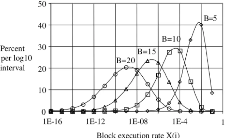
The execution rate after B random branches is computed. This process is repeated many times, and the number within each log10 interval of execution rate are counted.
The following figure shows the results of the simulation. 0 10 20 30 40 50
1E-16 1E-12 1E-08 1
Block execution rate X(i) Percent per log10 interval B=5 B=10 B=15 B=20 1E-4
Figure 1: Execution rate distribution for different branch depths
It can be seen that:
• for small values of B the distribution is skewed
• for larger B, the distribution seems to become closer to the log normal model and the spread increases
It follows from assumptions 1 and 2, that faults randomly located within the program structure should have execution rates that are typical of the overall execution rate profile. If the branching model is correct, these execution rates will be log-normally distributed. If there is a constant probability of failure per execution, (assumptions 3 and 4) the failure rates of the faults will also be log-normally distributed.
In fact it might not be necessary to assume a constant failure probability per execution (assumption 4). It would be sufficient if there was an independent distribution of failure probabilities per block execution. This would introduce another distribution into the product needed to compute the failure rate distribution. Given certain constraints on the new distribution, the result will still tend to a log-normal.
4.
Validation of the model assumptions
To check the assumptions inherent in the model, we implemented a validation test environment based on the “space” pre-processor program (PREPRO) [9]. This is an offline program written in C that was developed for the European Space Agency. The program computes parameters for an antenna array and is quite complex as it contains over 10 000 lines of non-commented code. The faults found within the code are documented and can be readily inserted for experimental purposes.A test-bed was developed to measure:
• the execution rate of each program block under a given profile
• the failure rates of the known program faults
• both of the above under a range of operational profiles To measure execution rates, we used the TCOV utility available on the Sun Solaris operating system. The instrumented version of PREPRO was run in a simple test harness written in Perl. This script invoked a random test data generator program (COPIA) which produces an input file for PREPRO. The test generator program was developed in [9] but has been adapted to take a “seed” value so that the pseudo random test sequence is repeatable.
To measure the basic block error rates under a given profile, a more complex test environment was developed. The PREPRO program contains a number of “define” statements which, if set, will result in the relevant fault being compiled into the program. The output of the erroneous program could be compared with an “oracle”, where no faults are compiled in.
We observed that the “oracle” program crashed in about 1% of test cases. As we were not in a position to identify the cause of these crashes, these test failures were excluded from later analyses of the failure rates of faults.
The random test generator COPIA uses an input table that can vary the probability of selecting the various
elements of the pre-processor input language. Different operational profiles were generated by altering the values in this table. We used two different profiles in our experiments (labeled P1 and P2).
4.1.
Comparison of the PREPRO execution rate
profile with a log-normal
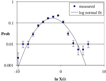
To assess whether the log normal is a good fit for execution rates, we computed the mean and variance of lnX over all basic blocks under profile P2. If the execution rates are log normally distributed, then the log-normal parameters would be µ = E(lnX) and σ = √Var(lnX). The distribution log execution rates are shown below together with the log-normal curve derived from the mean and variance. The results are shown in the figure below.
0.001 0.01 0.1 1 -10 0 10 ln X(i) Prob measured log normal fit
Figure 2: Distribution of ln X(i) (block execution rate) compared to a log normal fit (profile P2)
A Kolmogorov-Smirnov test gave a 93% probability that the observed execution rates were log-normally distributed. A similar result was obtained for profile P1. The predicted σ values are also fairly similar for both input profiles (2.5 and 2.4 for P1 and P2 respectively), even though the execution rates of individual blocks can change by an order of magnitude under the two profiles.
In some ways it is surprising the fit is so good. In particular, the peak value is skewed and greater than predicted, and the measured values can deviate markedly from the predicted value in the tails of the distribution. There are a number of possible explanations for these deviations:
• The program flow graph is not a simple tree structure. Inspection of the code shows that there is often a central code thread that diverges through multiple branches then recombines. This “beads on a string”
structure can affect the proportion of code at each branch depth, especially if the thread of central code is long compared to the side branches. The peak value occurs when X(i)=1. This suggests that there is a disproportionate amount of code in the central thread.
• The log-normal distribution prediction only applies at deep levels of nesting in the program structure; for shallow levels of nesting, the distribution is more skewed, and approximates to a power law when the branch depth is only one or two levels deep.
• The “branching tree” model assumes there are no loops or subroutine calls. This would imply that the block execution rate per test for a block is no more than unity. As rates of between 10 and 100 are observed in the distribution, this assumption is clearly invalid. On the other hand, variable execution rates due to loops and subroutines could be viewed as additional distributions that, under the central limit theorem, would also lead to a log-normal (but with rates greater than unity).
4.2.
“Typicality” of the execution rate of faulty
code blocks
It is assumed that the execution rates of faults are “typical”, i.e. are drawn randomly from the execution rate profile of program blocks. This would imply that there is a constant fault density throughout the code blocks, regardless of how deeply nested the code blocks are within the program. This assumption might be challenged because infrequently executed blocks might be more error-prone as they are less likely to be tested. On the other hand, module testing and code review work equally well at any depth, so there are reasons for believing that the fault density does remain constant.
If the assumption of a constant fault density is correct, the execution rate distribution of the known faults should be similar to that for all blocks in the program. To test this assumption, we measured the error rates in PREPRO under profile P2 for 28 of the known faults.
In Figure 3 below, the distribution of the execution rates of the faulty blocks is superimposed on the execution rate distribution for all accessible blocks. Note that “all accessible blocks” excludes the defensive code blocks that cannot be reached under the input profile. A Kolmogorov-Smirnov two-sample test was performed to compare the execution rate distributions of faulty blocks against all executed blocks. This showed there was a 42% chance they were drawn from the same distribution. So the hypothesis of “typicality” cannot be rejected at the 90% confidence level.
0 5 10 15 20 25 30 35 40 45 0.0001 0.001 0.01 0.1 1 10 100 1000 Execution rate (X) Percent Blocks per log10 interval Faulty blocks All blocks
Figure 3: Comparison of PREPRO execution rates: all blocks X(i) vs. faulty blocks X(j)
4.3.
Probability of failure per execution
Using the measurements of the probability of failure
λ(j) and execution rates X(j)of the faulty block j we could compute the probability of failure:
Pfail(j) = λ(j) /X(j)
The two distributions for Pfail for input profiles P1 and P2 are shown in the figure below.
0 2 4 6 8 10 12 14 0.01 0.03 0.1 0.3 1 Profile P1 Profile P2 P fail (j) Faults
Figure 4: Variation in the Probability of failure per block execution: Pfail(j)
Clearly Pfail is not the constant f assumed in the model. The study indicates that for profile P1, Pfail(j) can vary by two orders of magnitude, and the variance of ln(Pfail) is 0.69.
The analysis performed with the second operational profile P2 produced very similar results. This was observed even though the execution rates for specific blocks changed very significantly (an order of magnitude increase or decrease).
The result suggests that the distribution of block failure probabilities is independent of the block execution rates. A log-normal distribution will still be produced if we take a product of independent distributions of different types, provided no single distribution is “dominant”, i.e. the variance of any single distribution is much less than the variance of all distributions combined.
The block execution rates are close to log-normal (see Figure 2) and variance of logarithm of execution rates is around 2.4. Since the variance of ln(Pfail) is only 0.69, we infer that Pfail distribution is not dominant with respect to the execution rate distribution and hence we expect the product of these two distributions to be close to a log-normal.
4.4.
Distribution of failure rates
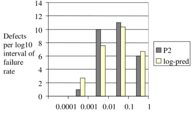
If we assume the execution rate has a log-normal distribution (shown by the solid line in Figure 2), and we take the Pfail distribution in Figure 5, we can take the product of these distributions to predict the expected failure rate distribution. Figure 5 compares the predicted failure rate distribution against the actual failure rate distribution observed under profile under profile P2.
0 2 4 6 8 10 12 14 0.0001 0.001 0.01 0.1 1 Defect failure rate λ(j) Defects per log10 interval of failure rate P2 log-pred
Figure 5: Failure distribution vs. log-normal prediction (profile P2)
It can be seen that the predicted distribution of failure is close to the observed distribution and lends support to the proposition that the failure rate distribution is likely to be log-normally distributed even if the failure probability per block execution is not constant.
5.
Extension to worst case bound theory for
log-normal distribution
The analysis in this paper and previous research [8] suggests that the distribution of failure rateswill be close to log normal. If we make an additional assumption that the failure rates of the faults have a log normal distribution we should be able to use equation (1) to derive a less pessimistic worst case bound. Unfortunately there is no analytic solution to reliability growth models based on a log-normal distribution. However for a worst case bound, we can apply Hölder’s inequality theorem [4] to establish a worst case bound for the integral of equation (1).
The log normal probability distribution function for the failure rate λ is:
σ
µ
−
λ
−
⋅
π
λσ
2 22
)
)
(ln(
exp
2
1
This is the equivalent of a normal distribution in log– linear space with the width of the distribution given by σ
and the “mean” by µ. The overall failure rate, θ, with this distribution is just the usual integral of λ, the total number of faults (N) and the probability distribution for λ:
θ =
λ
σ
µ
−
λ
−
⋅
π
λσ
λ
∫
∞d
2
)
)
(ln(
exp
2
0 2 2N
There is an analytic solution for this:
)
2
exp(
µ
σ
2θ
=
N
⋅
+
(2)This represents the failure rate of the program prior to testing, but we are particularly interested in how the mean failure rate after time t. This is given by:
λ
σ
µ
λ
π
σ
θ
λd
2
)
)
(ln(
exp
2
1
)
(
0 2 2 te
N
t
∞ −∫
⋅
−
−
=
(3)This integral is known to be mathematically intractable (see for example [8] and its absence from tables of integrals and transforms). The usual approaches of variable substitution and expansion do not lead to usable results. Although the integral for the variation of the mean failure rate with time is intractable we can obtain an approximation using a version of Hölder’s inequality [4] for integrals. This states that:
a b x f x( ) g x⋅ ( ) ⌠ ⌡ d a b x f x( )
(
)
p ⌠ ⌡ d
1 p a b x g x( )(
)
q ⌠ ⌡ d
1 q ⋅ ≤ (4) where:1
1
1
+
=
q
p
andp
>
1
If the exponential terms in (3) are substituted for f(x) and g(x) in (4), a bounding formula can be derived that is a function of p. It can then be shown that for the limiting case where p= 1, the following bound applies:
t
N
t
⋅
σ
⋅
π
≤
θ
2
)
(
(5) This is similar in form to the original bounding formula [2], i.e.:t
e
N
t
⋅
≤
θ
(
)
(6) The main difference is that (6) represents the worst case bound, regardless of the failure rate distribution, while (5) is a bound that assumes a log-normal distribution with a spread of σ. With this additional assumption about distribution, the Holder bound is normally less pessimistic as illustrated in the following table: e 2.7181
2
π
σ
σ
=
2.507
084
.
1
2
π
σ
σ
=
2.718
2
2
π
σ
σ
=
5.0143
2
π
σ
σ
=
7.520Table 1: Comparison of failure bound constants It can be seen that for σ< 1.084, the Holder bound is actually more pessimistic than the worst case bound formula. For complex software σ is typically 2 or 3 (see Table 2), so the Holder bound can be 2 or 3 times less pessimistic than the worst case bound while still remaining conservative.
As the N/e⋅t formula is the true worst case bound, we can combine the limits in (5) and (6) as follows:
)
2
,
max(
)
(
σ
π
⋅
≤
θ
e
t
N
t
(7)6.
Application of the theory
An example of the application of the bounding formulae to the Stratus 2 reliability growth data [8] is shown below. 10 4 10 5 10 6 10 2 10 3 10 4 10 5
Operating time (hours)
10
Log normal limit (t=0) Worst case (N/e.t) Holder bound log normal fit
MTTF (hours)
Figure 6: Comparison of MTTF predictions (Stratus 2 data)
Figure 6 shows the log normal fit using the N, σ and µ
values given in [8], the log normal integral (equation 3) was computed in Mathcad using numerical integration methods. The graph also shows the corresponding Holder and worst case bound predictions, together with the limiting value of the log normal integral at t=0 (derived from equation 1).
The Holder bound should be tangential to the log-normal fit at some point, so the long term prediction is quite accurate. The Holder bound only requires an estimate of σ, and as shown in the earlier simulation study, the spread of the failure rate distribution depends on program complexity and maximum branch depth in the program. In addition, analyses by [8] show there are quite consistent values of σ for different IBM and Stratus operating systems [8] as shown in Table 2.
Software σσ Stratus 1 3.28 Stratus 2 2.68 IBM product 2.1 3.27 IBM product 2.2 3.51 IBM product 2.3 3.44 IBM product 2.4 2.56 IBM product 2.5 3.50
Table 2: Sigma values for software products [8] While the actual size and complexity of these different products is not known, an operating system is likely to contain at least 1000 kilo lines of code (kloc). By contrast, we have shown earlier that the σ value for PREPRO, with around 10 kloc, is only 2.2. It may therefore be feasible to make a priori estimates of σ (as well as N) based on empirically derived relationships between σ and code size. In addition, if we can estimate µ, then the full reliability growth equation (3) can be used to estimate the reliability using numerical methods. This is discussed further in next section.
7.
Estimation of log-normal parameters
If reasonably good estimates of N and σ exist, and we can also measure the failure rate at t=0, θ0, equation (2)can be used to obtain an estimate for µ, i.e.:
−
=
)
2
exp(
ln
θ
0σ
2µ
N
(8)There is an extensive literature on methods for estimating N (which typically scale fairly linearly with the number of lines of code [5, 6, 7]). However we also need to estimate the σ parameterwith sufficient accuracy to make long term reliability predictions
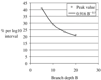
If we take the results of our simulation study in Figure 1, and plot the peak value against branch depth B, we observe empirically that there is a square root relationship as shown in Figure 7 below.
0 5 10 15 20 25 30 35 40 45 0 10 20 30 Branch depth B % per log10 interval Peak value 0.916 B− 0.5
Figure 7: Empirical relation between peak value and branch depth B
As we know that for a log normal distribution the peak value is proportional to 1/σ- (see equation 3), the spread
of the log normal distribution (σ) appears to be proportional to the square root of B. Empirically, the constant of proportionality is 0.916 per log10 interval of
failure rate. For a log-normal distribution, the peak value for the loge interval at the peak holds 1/√(2π)σ of the
faultsso, rescaling, the empirical relationship is:
B
B
0
.
84
2
)
10
ln(
916
.
0
⋅
=
=
π
σ
(9)For the simulation is Section 2, we assumed a single binary tree structure tree as illustrated below.
B=0
B=1 B=2
Figure 8: Single branching tree program model In this case, the number of blocks at branch level B is 2B and the total number of branches is 2B−1. If we know
the total number of branches in the program is nB, we can
infer that the maximum branch depth B for the program is:
)
(
log
2n
BB
≈
Substituting into equation (9):
)
(
log
84
.
0
2n
B≈
σ
However this is based on an unrealistic model of program structure. If we examine actual program structures, we see that the structure is often more like “beads on a string” as illustrated in Figure 9 below:
Figure 9: “Beads on a string” flow graph
If there are b beads on the string, effectively there are b separate subnets containing nB/b branches each, hence:
)
/
(
log
84
.
0
2n
Bb
≈
σ
(10)An example of the effect of beads on the expected value of sigma is shown in Table 3 below.
Number of beads (b) Number of Branches (nB) 1 10 100 1000 1000 2.66 2.17 1.53 0.00 10 000 3.07 2.66 2.17 1.53 100 000 3.43 3.07 2.66 2.17 1 000 000 3.76 3.43 3.07 2.66 10 000 000 4.06 3.76 3.43 3.07
Table 3: Predicted σ values
It can be seen that the predicted σ values are close to those given in Table 2. For example, if a typical operating system contained a million lines of code, and there was a decision every 10 lines, the number of branches would be nB=100 000, so a σ value range from 2.67 to 3.44 would
be expected (depending on the value of b). This is in reasonable accord with the measured σ values in Table 2 where the values range from 2.5 to 3.50.
We can also compare the predicted σ value against the results of the PREPRO analysis in Section 4. Here we know that the program size is 10 000 lines, and an analysis of the code indicates there are around 600 branch points and the average number of beads is unlikely to be greater than 10. From equation (10) we would expect σ
compared with the log-normal fit to the execution rate distribution where the fitted values for σ lie between 2.4 and 2.5.
8.
Discussion
This paper uses the central limit theorem to assert that a log-normal distribution failure rate should arise naturally from the program structure. In theory, the pre-conditions for a log-normal may not exist if there is a “dominant” distribution in the product of terms. Empirically, the actual distributions observed in our PREPRO analysis and prior research [8] suggest that log-normal distributions do arise in practice.
The program structural model used is relatively simplistic as it does not model subroutine calls and loops. Given the incomplete nature of the model it is surprising that the σ estimates are close the measured results. However the omission of subroutines and loops might not have a major effect. Multiple subroutine calls increases the total execution rate of the subroutine, and (in execution rate terms) moves the subroutine closer to the top of the tree. For example, a subroutine call in every “leaf” of the tree is equivalent to having the subroutine subnet executed once per test. Loops increase the execution rate of blocks within the loop subnet, and hence shift the block execution rate distribution “to the right” but the subnet distribution rates are still log-normal distributed. For example, in Figure 4, block execution rates can exceed 100 per test (due to internal loops), but the overall distribution is still close to a log-normal
Given the approximations inherent in the branch model we cannot be sure that equation (10) is generally applicable. However the equation suggests that σ is relatively insensitive to program size and structure. This could explain the remarkable level of consistency observed in the Adams reliability data [1] for IBM operating systems. This high level of consistency could simplify the process of estimating the log-normal parameters (e.g. it may be possible to use generic σ values for particular types and sizes of programs).
Given the relatively small changes in σ predicted theoretically (and observed in practice), it should be feasible to use the Holder bound (equation 5) rather than the more pessimistic worst case bound (equation 6). Both of these bounding equations can still be pessimistic for small values of t. A better reliability prediction we use the full log-normal integral (equation 3). We can estimate µ
using equation (10), but this requires more accurate estimates for σ to correctly model the growth curve. For example, an error of 10% error in a σ estimate of 3, changes the failure rate “peak” of the log-normal distribution by a factor of two. If the parameter
uncertainties are large, it is probably safer to use the Holder bound.
9.
Conclusions and further work
Prior research suggests that a log-normal failure rate distribution is likely to exist in software. We have put forward a specific software failure model that leads to log-normal distribution of failure rate for software faults (given software of sufficient complexity).
The assumptions underlying the model have been evaluated on a relatively small program, and this seems to support the hypothesis that block execution rates and the failure rate of faults will follow a log-normal distribution.
If failure rates are log-normally distributed, we can derive less pessimistic worst case bound predictions for reliability growth. If we could obtain a realistic prior estimate of the log-normal parameters (σ and µ) then more realistic growth predictions would be possible.
Based on our branching tree model we have derived an equation that predicts an increase of σ as the branch depth increases (roughly as the square root of the maximum branch depth). While the branching tree model does mot include all the structures present in actual programs, the predicted σ values are fairly consistent with the values derived in [8] and our own internal study of the PREPRO software. Further work is needed to:
1. Check the hypothesis of log-normally distributed execution rates and defect failure rates.
2. Establish whether there is predictable relationship between the log-normal distribution parameters and program structure.
10.
Acknowledgements
This work was funded by the UK (Nuclear) Industrial Management Committee (IMC) Nuclear Safety Research Programme under British Energy Generation UK contract PP/114163/HN with contributions from British Nuclear Fuels plc, British Energy Ltd and British Energy Group UK Ltd. The paper reporting the research was produced under the EPSRC research interdisciplinary programme on dependability (DIRC).
References
[1] E.N. Adams, “Optimising Preventive Maintenance of Service Products”, IBM Journal of Research and Development, Vol. 28, No. 1, Jan. 1984.
[2] P.G. Bishop and R.E. Bloomfield, “A Conservative Theory for Long-Term Reliability Growth Prediction”, IEEE Trans. Reliability, vol. 45, no. 4, pp 550-560, Dec. 1996.
[3] P.G. Bishop, “ Rescaling Reliability Bounds for a New Operational Profile”, International Symposium on Software Testing and Analysis (ISSTA 2002), (Phyllis G. Frankl, Ed.), ACM Software Engineering Notes, vol. 27 (4), pp 180-190, Rome, Italy, 22-24 July, 2002.
[4] G.H. Hardy, J.E. Littlewood, G. Polya, “ Hölder's Inequality and Its Extensions”, Sections 2.7 and 2.8 in Inequalities, 2nd ed. Cambridge, England: Cambridge University Press, ISBN: 0521358809, pp. 21-26, 1988. [5] J.R. Gaffney, “Estimating the Number of Faults in Code”, IEEE Trans. Software Engineering, vol. SE-10, no. 4, 1984.
[6] T.M. Khoshgoftaar and J.C. Munson, “Predicting software development errors using complexity metrics”, IEEE J of Selected Areas in Communications, 8(2), pp 253-261, 1990.
[7] Y.K. Malaiya and J. Denton, “Estimating the Number of Residual Defects”, HASE'98, 3rd IEEE Int'l High-Assurance Systems Engineering Symposium, Maryland, USA, November 13-14, 1998.
[8] R.E. Mullen, “The Lognormal distribution of Software Failure Rates: Origin and Evidence”, Proc 9th International Symposium on Software Reliability Engineering (ISSRE 98), 1998
[9] A. Pasquini, A.N. Crespo and P Matrella, “Sensitivity of reliability growth models to operational profile errors”, IEEE Trans. Reliability, vol. 45, no. 4, pp 531–540, Dec. 1996.
![Figure 6 shows the log normal fit using the N, σ and µ values given in [8], the log normal integral (equation 3) was computed in Mathcad using numerical integration methods](https://thumb-us.123doks.com/thumbv2/123dok_us/36792.2505174/6.918.91.451.338.563/figure-integral-equation-computed-mathcad-numerical-integration-methods.webp)