Jason Roderick Donaldson,
Eva Micheler
Resaleable debt and systemic risk
Article (Accepted version)
(Refereed)
Original citation: Donaldson, Jason, Roderick and Micheler, Eva (2017) Resaleable debt and systemic risk.Journal of Financial Economics. ISSN 0304-405X
DOI: 10.1016/j.jfineco.2017.12.005
© 2017 Elsevier
This version available at: http://eprints.lse.ac.uk/68068/ Available in LSE Research Online: January 2018
LSE has developed LSE Research Online so that users may access research output of the School. Copyright © and Moral Rights for the papers on this site are retained by the individual authors and/or other copyright owners. Users may download and/or print one copy of any article(s) in LSE Research Online to facilitate their private study or for non-commercial research. You may not engage in further distribution of the material or use it for any profit-making activities or any commercial gain. You may freely distribute the URL (http://eprints.lse.ac.uk) of the LSE Research Online website.
This document is the author’s final accepted version of the journal article. There may be differences between this version and the published version. You are advised to consult the publisher’s version if you wish to cite from it.
RESALEABLE DEBT AND SYSTEMIC RISK
∗
Jason Roderick Donaldson
†Washington University in St Louis
Eva Micheler
‡London School of Economics
11 August 2016
Abstract
Many debt claims, such as bonds, are resaleable, whereas others, such as repos, are not. There was a fivefold increase in repo borrowing before the 2008 crisis. Why? Did banks’ dependence on non-resaleable debt precipitate the crisis? In this paper, we develop a model of bank lending with credit frictions. The key feature of the model is that debt claims are heterogenous in their resaleability. We find that decreasing credit market frictions leads to an increase in borrowing via non-resaleable debt. Borrowing via non-resaleable debt has a dark side: it causescredit chains to form, since if a bank makes a loan via non-resaleable debt and needs liquidity, it cannot sell the loan but must borrow via a new contract. These credit chains are a source of systemic risk, since one bank’s default harms not only its creditors but also its creditors’ creditors. Overall, our model suggests that reducing credit market frictions may have an adverse effect on the financial system and may even lead to the failures of financial institutions.
Keywords: resaleable debt, systemic risk, bankruptcy, repos, securities law
JEL Classification Numbers: G21, G28, G33, K12, K22
∗The support of the Economic and Social Research Council (ESRC) in funding the Systemic Risk Centre is gratefully acknowledged [grant number ES/K002309/1]. Thanks to Gaetano Antinolfi, Bruno Biais, Jen Dlugosz, Armando Gomes, Radha Gopalan, Dalida Kadyrzhanova, Mina Lee, Giorgia Piacentino, Adriano Rampini, Matt Ringgenberg, Edmund Schuster, Ngoc-Khanh Tran, Ed Van Wesep, and Jean-Pierre Zigrand for comments.
1
Introduction
Credit frictions decreased substantially in the decades leading up to the 2008 financial crisis.1 This coincided with the expansion of repo markets, which grew fivefold between 1990 and 2007. Before the crisis, the value of outstanding repos in the US exceeded five trillion USD.2 The markets appeared to be functioning well, allowing banks to find cheap, short-term liquidity. However, they were harboring systemic risk, because banks were exposed to one another in credit chains. This meant that if one bank defaulted, it harmed not only its immediate creditors, but potentially its creditors’ creditors as well. This systemic risk manifested itself in the financial crisis, in which shocks to a relatively small set of assets threatened to bring down the entire financial system. Did the buildup of systemic risk relate to the decrease in credit frictions? In general, can a decrease in credit frictions cause an increase in systemic risk?
In this paper, we construct a corporate finance-style model to address this question. We find that the answer is yes. Our main result is that a decrease in credit frictions increases systemic risk. This is because the decrease in credit frictions leads credit chains to become more widespread, and these credit chains harbor systemic risk.
The key novel ingredient in our model is the heterogeneous resaleability of debt claims. For concreteness, consider the salient examples of bonds and repos. Bonds are resaleable, whereas repos are not.3 As a result, lending via repos leads to credit chains, whereas lending via bonds does not. To see this, suppose you are a lender—you have a loan on the asset side of your balance sheet—and you suddenly need liquidity. Your options for raising this liquidity are different if you hold a bond than if you hold a repo. If you hold a bond you can sell it in the market. In contrast, if you hold a repo, you cannot sell it. Hence, you obtain liquidity by borrowing via a new repo. This creates a credit chain, because you are now not only a creditor in the original repo, but a debtor in the new repo as well. In summary, when you hold a non-resaleable instrument such as a repo, the result is a credit chain. This brings with it systemic risk, since defaults can transmit through the chain.
1
Low credit market frictions in the US before the crisis reflected a number of factors, including advanced information technology for execution and settlement, low transaction costs (Domowitz, Glen, and Madhavan (2001), Jones (2002)), relatively low information asymmetries (Bai, Philippon, and Savov (2012), Greenwood, Sanchez, and Wang (2013)), and a number of potential legal factors, such as privileged bankruptcy treatment of some bank liabilities (Morrison, Roe, and Sontchi (2014)) and required financial disclosure (La Porta, Lopez-De-Silanes, and Shleifer (2006)).
2
See Homquist and Gallin (2014).
3
That bonds are resaleable and repos are not is a formal legal property of these claims. Other financial claims, such as derivatives, are also not resaleable; we comment on our model’s applicability to derivative markets in Subsection 1.1.
How does a change in credit frictions affect your choice whether to lend with a bond or a repo? In our model, a decrease in credit frictions makes you relatively more likely to lend via a repo. This is due to the fact that when you are an intermediate link in a credit chain, there are two contracts that must be enforced, one between you and your creditor and another between you and your debtor. Thus, you bear the costs of credit frictions twice, once for each contract. If frictions are high, you have a strong incentive to avoid these double costs. To do this, you lend via resaleable debt like bonds. In this case, no credit chain is formed and systemic risk is low. On the other hand, if credit frictions are low, you have a weaker incentive to avoid the costs of credit chains. You may prefer to lend via non-resaleable debt like repos. In fact, in reality, you have a strong incentive to use repos instead of bonds: repos are exempt from the automatic stay in bankruptcy and thus they are effectively super-senior claims.4 When credit frictions are low, the value of this super-seniority outweighs the cost of the double incidence of credit frictions. As a result, credit chains form and systemic risk is high. This is the essence of our main result: decreasing credit market frictions can increase systemic risk. The reason is that decreasing credit frictions makes it is less likely that banks issue resaleable debt and, hence, more likely that credit chains form.
Model preview. We now describe our model and results in more detail. We model the interbank market within a classical corporate finance framework. At the core of the model is one financial institution, which we call Bank A, that needs to raise finance in order to scale up a project. Bank A borrows from a competitive creditor, which we call Bank B. Bank A can borrow via one of two instruments, a bond or a repo.5 As discussed above, a bond is resaleable whereas a repo is not. The amount that a bank can borrow is limited by the assets it can pledge, via a standard limit to pledgeabity. Specifically, the repayment a bank makes to its creditor cannot exceed a fixed fraction θ of the bank’s assets. This fraction θ, which we refer to as the“enforceability” in the economy, captures credit frictions. An increase in enforceability θ corresponds to a decrease in credit frictions. At an interim date, after Bank B has made the loan to Bank A, it may suffer a “liquidity shock,” i.e. it may suddenly need cash. If Bank B suffers a liquidity shock, it raises liquidity in the interbank market from a third financial institution, which we call Bank C. Specifically, Bank B raises this liquidity either by selling Bank A’s bond to Bank C or by entering a new repo agreement with Bank C.
4
See footnote 15 for a discussion of the special treatment that repos receive in bankruptcy.
5
We use the labels repo and bond throughout for non-resaleable and resaleable instruments, respectively. Note that when we think about short-term bank funding, the kind of bond we have in mind is commercial paper. We discuss the applicability of our model to short-term bank funding further in Subsection 1.1 and to more general abstract settings in Subsection 4.2.
Bank B’s Sale of Bank A’s Bonds to Bank C
Bank A
A’s debt to B A’s debt to C
θ
C buys A’s bondsBank B Bank C
Figure 1: Because bonds are resaleable, Bank B obtains liquidity by selling Bank A’s bonds to Bank C. No credit chain emerges.
Bonds are attractive relative to repos because they are resaleable. However, re-pos are attractive relative to bonds because they are effectively senior to bonds in bankruptcy. Thus, when Bank A borrows in the interbank market, it trades off the resaleability benefit of bonds against the seniority benefit of repos.
For most of our analysis, we focus on this trade-off in the interbank market, but we generalize our model in Subsection 4.2. There, we relax the assumption that non-resaleable debt claims (repos) are senior to non-resaleable debt claims (bonds). Specifically, we model general debt markets following Kiyotaki and Moore (2005) and show that our main results are broadly applicable. For example, this analysis may cast light on a borrower’s choice whether to fund itself via a bank loan (non-resaleable) or long-term bonds (resaleable).
Results preview. First consider the case in which Bank A borrows from Bank B via a bond. In this case, when Bank B suffers a liquidity shock, it sells Bank A’s bond to Bank C. This sale is depicted in Figure 1. Observe that Bank A now has a debt to Bank C directly. There is no credit chain. There is only one contract to be enforced, the debt from Bank A to Bank C. Credit frictions kick in only once and Bank A’s debt capacity is (roughly) proportional to the enforceability θof this contract.
A Credit Chain from Bank A to Bank B to Bank C Bank A A’s debt to B
θ
Bank B B’s debt to Cθ
Bank CFigure 2: A credit chain emerges when Bank A borrows from Bank B via repos. case, when Bank B suffers a liquidity shock, it must enter into a new contract to find liquidity—because Bank A’s repo debt is not resaleable, Bank B cannot liquidate it in the market. Thus, Bank B borrows from Bank C via a new repo contract. This is depicted in Figure 2. Observe that Bank A has debt to Bank B and Bank B has debt to Bank C. There is a credit chain. There are two contracts to be enforced. Credit frictions kick in twice, once at each link in the credit chain, and Bank A’s debt capacity is (roughly) proportional to the enforceabilitysquared orθ×θ. Intuitively, there is one θfor each of the two contracts.
Now consider how an increase in enforceability affects Bank A’s choice between bonds and repos. Asθ increases, the amount Bank A can borrow with bonds increases linearly and the amount Bank A can borrow with repos increases quadratically. In other words, the sensitivity of Bank A’s debt capacity to enforceability is higher when it borrows via repos than when it borrowers via bonds. Thus, as credit frictions decrease, Bank A switches from bond borrowing to repo borrowing.
What are the implications of increasing enforceability for systemic risk? We have just established that increasing enforceability leads Bank A to borrow via repos and that this, in turn, leads to credit chains. Credit chains harbor systemic risk because if Bank A defaults on its debt to Bank B, Bank B may default on its debt to Bank C. In our model, such default cascades can arise only when enforceability is high, because that is when Bank A funds itself with repos and credit chains emerge. Note that even
though increasing enforceability improves the functioning of each market individually, it may have an adverse effect on the system as a whole, causing an increase in systemic risk.
Further results. In the baseline model, we make the simplifying assumption that Bank A’s project itself serves as collateral, even though repos and commercial paper are typically collateralized by financial securities in reality.6 In an extension, we modify the model so that Bank A pledges securities to fund an illiquid project. We show that our main results are robust to the use of securities as collateral. However, the analysis also raises an important question: why would Bank A prefer to use the securities as collateral to borrow rather than to sell them in the market, avoiding the effects of credit frictions? We provide a formal explanation based on heterogenous beliefs and find that if Bank A believes the securities are undervalued by the market, it will use them as collateral rather than sell them.7
We also explore six other extensions of our baseline model. This analysis affirms the robustness of our main findings and provides new results. First, we show that our model can be applied to many debt markets, not only to the interbank market. In particular, our main results are robust to relaxing the assumption that non-resaleable debt (repos) is senior to resaleable debt (bonds). Second, we consider Bank A’s maturity choice in the presence of roll-over risk. We find conditions under which Bank A matches the maturity of its liabilities to the maturity of its project, as we assume exogenously in the baseline model. Third, we consider the possibility that credit chains may have more than two links. We show that longer chains make repo borrowing relatively less attractive. However, our qualitative findings do not change. Fourth, we ask how systemic risk is affected by a relatively short-term stay on repos, rather than a full exemption from stays. We show that a short-term stay is preferable to an exemption in our setting, but that longer stays for repos are even better. Fifth, we consider how a tax on repo borrowing affects systemic risk. We find that debt capacity is convex in the tax rate, suggesting that a small tax may have a relatively large effect on the volume of repo borrowing. Finally, we do a reduced-form welfare analysis. We explain that if bank default is socially costly, then increasing systemic risk corresponds to decreasing social welfare.
Policy. Our model is stylized, but may still cast light on policy debate. Should
6
Our baseline assumption may be realistic if Bank A’s project is a financial investment—i.e. if Bank A is buying securities on margin—as discussed in Subsection 4.1.
7
There are also institutional reasons that Bank A may prefer to use securities as collateral rather than sell them; for example, it may need to maintain ownership of the securities to meet regulatory liquidity or capital requirements.
repos maintain their special treatment in bankruptcy? The exemption from automatic stays for repos makes repos more desirable to Bank A. Thus, the exemption leads Bank A to undertake more repo borrowing and, hence, leads to more credit chains. Since these credit chains are the source of systemic risk in the model, the exemption from the stay exacerbates systemic risk. This finding contrasts with the arguments ad-vanced by proponents of the exemption, who suggest that the safe harbors are “effective in...limiting [counterparties’] exposure to possibly catastrophic losses from the failure of the debtor. This is the very reason why Congress enacted the safe harbors in the first place” (Exploring Chapter 11 Reform (2014)).
Our findings also affirm that regulators must take a macro-prudential approach, as decreasing credit frictions makes every market function better individually, but makes the system as a whole more dangerous.
Layout. The remainder of the paper is organized as follows. There are two remain-ing subsections in the Introduction, first, a discussion of the realism of our assumptions and the empirical relevance of our results and, second, a review of related literature. Section 2 presents the model. Section 3 contains the formal analysis. In Section 4, we derive further results by extending the model to include the financial securities as collateral, more general instruments, rollover risk, longer chains, short-term stays for repos, taxes on repos, and social costs of bank default. In Section 5, we conclude and consider policy implications. Appendix A contains omitted derivations and proofs. 1.1 Realism and Empirical Evidence
While our model is stylized, we believe that our baseline model provides a useful approx-imation of the interbank market, with reasonable assumptions and predictions. Here we discuss these briefly in connection with empirical work. First, we point out that repos and asset-backed commercial paper (a type of bond) are relatively substitutable instru-ments for short-term bank funding. This is because they both have relatively short ma-turities and they are often secured by similar collateral (Krishnamurthy, Nagel, and Orlov (2014)). Second, we suggest that the bankruptcy advantage of repos is important, as repo volume increased after Congress introduced the safe harbor provision (Garbade (2006)). Third, we emphasize that credit chains are an important feature of the repo market (repo chains are typically associated with the so-called “rehypothecation”8 of collateral, see Singh and Aitken (2010) and Singh (2010)). Banks assume offsetting long and short repo positions, even though many repos are very short-term and it may
8
Since a repo contract is formally the sale and repurchase of assets, not the pledging (or “hypothecating”) of collateral, the term “rehypothecation” is not favored by lawyers.
seem that they should be “self-liquidating.” This may be because banks manage liquid-ity over very short time horizons, taking offsetting positions within each day. Another reason for this may be that many repos are of longer maturities, with an estimated thirty percent of repos having maturity longer than a month (Comotto (2015)). Fi-nally, many repos have “open” tenors, with no specified maturity. These are typically thought about as overnight contracts, but a lender in an open repo must give its coun-terparty notice before closing the contract; sometimes several weeks’ notice is required (Comotto (2014)).
In our baseline model, we focus on credit chains in the interbank lending market, but our model may also be applied to financial derivatives. In the derivatives market, the analogy to the trade-off between junior, resaleable bonds and senior, non-resaleable re-pos is the trade-off between standardized, exchange-traded derivatives and specialized, OTC derivatives. Exchange-traded derivatives have the advantage of being resaleable. Therefore, they do not lead to the formation of chains of counterparties. In contrast, OTC derivatives have the advantage of being customizable, and they have the potential advantage of providing insurance against specialized risks. Just as decreasing credit frictions makes credit chains relatively less costly in the baseline model, decreasing credit frictions makes risk-management chains relatively less costly here. Thus, when credit frictions are low, OTC derivatives are relatively popular and risk-management chains are relatively widespread: decreasing credit frictions can increase systemic risk in derivatives markets just as it can in funding markets. Further, derivatives markets grew even more dramatically than repo markets in the years before the 2008 crisis. The notional value of all financial derivatives contracts was estimated at 766 trillion USD in 2009, a three hundred-fold increase from thirty years earlier (Stulz (2009)). Repos and derivatives often constitute a larger fraction of banks’ balance sheets than bonds of all maturities combined. For example, in 2009 over forty-five percent of Barclay’s liabilities were listed as “repurchase agreements and stock lending” (199 billion GBP) or “derivatives” (403 billion GBP) on its balance sheet.9
Our application to the interbank market depends on the assumption that there are frictions in the interbank market. In particular, we assume that there is limited enforceability of contracts or, equivalently, limited pledgeability of cash flows. The assumption is standard in the theory literature—for example, Homstrom and Tirole
9
Barclay’s annual reports are available online here <https://www.home.barclays/barclays-investor-relations/ results-and-reports/annual-reports.html>. The Royal Bank of Scotland reports similar numbers (see <http://investors.rbs.com/annual-report-subsidiary-results/2010.aspx>). The corresponding figures are hard to find for US banks, since they classify their derivatives holdings as risk management instruments and, therefore, are not required to list them on their balance sheets.
(2011) make the assumption and provide a list of “several reasons why this [limited enforceability] is by and large reality” (p. 3). We think that the realism of the assump-tion for our applicaassump-tion is demonstrated by the importance of collateral in interbank contracts (Bank for International Settlements (2013))—if there were no pledgeablity frictions, banks would not need to post collateral at all. In addition, the years-long bankruptcy proceedings of Lehman Brothers demonstrated that bank creditors can face severe frictions when trying to claim repayment. Further, we point out that our model does not rely on the assumption that contractual enforceability is weak, but only on the assumption that it is imperfect, which we believe it is for all contracts in practice.
Finally, to emphasize the empirical importance of the problem we study, we remark that several papers suggest that the systemic risk that built up in the repo market may have played an important role in the financial crisis of 2008–2009 (Copeland, Martin, and Walker (2014), Gorton and Metrick (2010), Gorton and Metrick (2012), Krishnamurthy, Nagel, and Orlov (2014)).10
1.2 Related Literature
Kiyotaki and Moore (2000) also analyze how the resaleability of debt claims can mit-igate the allocational inefficiencies that stem from limits to enforceability.11 They demonstrate that a small amount of resaleability (or “multilateral commitment”) can substitute for a substantial lack of enforceability (or “bilateral commitment”) in a deter-ministic, infinite-horizon economy. Rather than focus on allocational efficiency as they do, we study borrowers’ endogenous choice of instruments and analyze the implications for systemic risk. Our analysis points to a potential dark side of enforceability that is not present in Kiyotaki and Moore’s deterministic setting.
In another 2001 paper, Kiyotaki and Moore study credit chains. Rather than study the transferability of debt, that paper shows how chains of bilateral borrowing can emerge and, as such, it constitutes an early contribution to the growing literature on financial networks. Many papers in this literature study systemic risk, including Acemoglu, Ozdaglar, and Thabaz-Salehi (2013), Allen, Babus, and Carletti (2012), Allen and Gale (2000), Blumh, Faia, and Krahnen (2013), Cabrales, Gottardi, and Vega-Redondo (2013), Elliott, Golub, and Jackson (2014), Gale and Kariv (2007), Glode and Opp (2013), Rahi and Zigrand (2013), and Zawadowski (2013). In only a few of these papers, however, is the equilibrium network endogenous. An emerging
10
Note that these papers differ in their conclusions about theway in which repos contributed to the crisis.
11
In this paper, Kiyotaki and Moore develop a framework that they explore further in subsequent work, including Kiyotaki and Moore (2001a), Kiyotaki and Moore (2005), and Kiyotaki and Moore (2012).
theory literature takes a detailed approach to modeling credit chains in the repo market specifically, including Kahn and Park (2015), Infante (2015), and Lee (2015).
Numerous other papers study the circulation of private debt, including Gorton and Pennacchi (1990), Gu, Mattesini, Monnet, and Wright (2013), Kahn and Roberts (2007), and Townsend and Wallace (1987). These papers typically do not consider debt resaleability as a choice of the borrower and, therefore, they do not study the implications of this choice for systemic risk.
We also hope to contribute to the debate surrounding the bankruptcy seniority of repos and derivatives. Relevant papers in this literature include Antinolfi, Carapella, Kahn, Martin, Mills, and Nosal (2014), Bliss and Kaufman (2006), Duffie and Skeel (2006), Edwards and Morrison (2005), Lubben (2009), Roe (2011), and Skeel and Jack-son (2012). Notably, Bolton and Oehmke (2014) bring a corporate finance model to bear on the question of bankruptcy seniority, but they focus on the exemptions for derivatives.
2
Model
In this section we set up the model, outlining the players and their technologies, the debt instruments by which they can borrow, the specific nature of limited enforcement, and the timing of moves. We also include a subsection describing several restrictions that we impose on parameters.
2.1 Players and Technologies
There is one good called cash. There are three dates Date 0, Date 1, and Date 2. The time between Date t and Date t+ 1 is called “overnight.” Cash is the input of production, the output of production, and the consumption good. The main actor in the model is a risk-neutral bank called Bank A. Bank A has an endowment ofepounds and a risky constant-returns-to-scale technology. The technology takes two periods to produce, starting at Date 0 and terminating at Date 2. It has random gross return R˜, which isRH with probability π andRL< RH with probability 1−π. Figure 3 depicts
the technology. We call the event that R˜ =RH “success” and the event thatR˜ =RL
“failure.” Denote the expected return by R¯ :=πRH + (1−π)RL.12
12
Note that we think about π as rather large so that failure is an extreme event. In the repo market, failure should be interpreted as the joint event in which Bank A’s project fails and the value of its pledged collateral is not sufficient to cover its loan. We do not model this collateral explicitly here, but we discuss it in the extension in Subsection 4.1.
−(e+IA)
π
(e+IA)RH (success)
1
−
π
(e+IA)RL (failure)
Figure 3: Depiction of Bank A’s technology.
Bank A funds its investment by borrowing capital I from a competitive market of risk-neutral banks. The project is scaleable, so the quantity I is determined in equilibrium. We model the competitive market in reduced form by having Bank A make a take-it-or-leave-it offer to borrow from a second risk-neutral bank, Bank B. Bank B breaks even in expectation but its preferences are uncertain: with probability 1−µ Bank B values consumption only at Date 1 and with probabilityµit values consumption only at Date 2 (all random variables are pairwise independent). To be more specific, with probability 1−µBank B lexicographically prefers Date 1 consumption to Date 2 consumption; with probability µBank B lexicographically prefers Date 2 consumption to Date 1 consumption.13 We call the event that a bank wishes to consume at Date 1 a “liquidity shock.” The inclusion of the possibility that a bank is hit by a liquidity shock is a simple way to generate a motive to trade in a secondary market before Bank A’s debt matures—when hit by a liquidity shock, Bank B wishes either to resell Bank A’s debt or to borrow against Bank A’s debt to satisfy its liquidity needs at Date 1. Rather than viewing Date 1 as a fixed point in time that the banks know in advance, we interpret it as a random time at which Bank B needs liquidity. Thus, since the arrival time of Bank B’s liquidity shock is uncertain at Date 0, Bank A cannot borrow with a contract that matures exactly when Bank B suffers the liquidity shock. We discuss
13
The lexicographic preferences are just a modelling device that induces Bank B to have well-defined preference for more to less at Date 2 even if it is hit by a liquidity shock at Date 1; this is important only in the details of micro-founding enforcement constraints (see Subsection 2.3 below).
Date 0
Bank A returnsR˜
Date 1 Date 2
Bank A borrows from Bank B Bank B suffers liquidity shock Repayment
Bank B obtains liquidity from Bank C
Figure 4: Timeline when Bank B suffers a liquidity shock. this further in Subsection 4.3.
For simplicity, we assume that Bank B has deep pockets at Date 0. By “deep pockets” we mean that it has sufficient cash to fund Bank A at Date 0 so that Bank A does not need to find a second creditor. If Bank B is hit by a liquidity shock, it uses all this cash to generate liquidity at Date 1. We discuss the role of assets in place further in Subsection 4.1.
There is a competitive interbank market open at Date 1, in which banks buy and sell bonds in the secondary market as well as borrow and lend among themselves. We model this by allowing Bank B to obtain funds from a third risk-neutral bank, Bank C. Bank B can either sell Bank A’s debt or borrow against it. Again, competition is captured by assuming that Bank B makes Bank C a take-it-or-leave it offer, whether to sell bonds or to borrow against repos.
Figure 4 depicts the timing described here for the case in which Bank B suffers a liquidity shock. Subsection 2.4 below gives a more formal description of the timing. 2.2 Borrowing Instruments
The crux of the model is the trade-off between borrowing via abilateral contract called a repo and borrowing via a resaleable instrument called a bond. In the model, two features distinguish repos from bonds. The first feature is that bonds are resaleable. A bank that buys a bond can sell it to another bank in the Date-1 market. The issuer of the bond repays its bearer at maturity, regardless of whether this bearer was the original owner at Date 0. Repos, in contrast, are not resaleable. A repo must be settled by the writer and its counterparty. The second feature that distinguishes repos from
bonds is that repos are not stayed in bankruptcy.14 The counterparty to a repo recoups its debt immediately, even if its counterparty defaults. The counterparty to a bond, in contrast, must wait to liquidate until it is awarded the assets in the bankruptcy proceedings.15 To capture the costs of waiting to liquidate, we normalize bondholders’ liquidation value to zero in the event of default.16 We assume that the realization of
˜
R is not verifiable, so state-contingent contracts are impossible.17 Thus, as in reality, both bonds and repos are debt contracts, i.e. promises to repay a state-independent face value in the future in exchange for cash today. We summarize the dimensions along which repos and bonds differ in Figure 5.
A main question we ask is under what conditions Bank A will fund its Date 0 investment via repos as opposed to bonds. When Bank A determines its funding in-strument, it will face a trade-off in borrowing costs. Repos decrease borrowing costs because creditors have higher recovery values in the event of default; in contrast, bonds reduce borrowing costs because they may come with a liquidity premium. This liquid-ity premium is a result of the fact that lenders can sell them at Date 1 to meet their liquidity needs when they suffer liquidity shocks. That is to say, borrowers trade off bonds’ resaleability against repos’ super-seniority.
2.3 Limited Enforcement
The key friction in the economy is limited enforcement. We assume that creditors cannot extract all of a project’s surplus when they collect on their debts. In particular, there is an exogenous number θ∈ (0,1) that gives an upper bound on the proportion
14
As mentioned in the Introduction, this specific assumption of seniority is not essential for our main results, as we discuss in Subsection 4.2.
15
The special treatment of repos is a feature of the US Bankruptcy Code. It is a legal advantage of repos, which are formally not debt contracts but are rather sales and repurchases of securities. In the event of a debtor’s bankruptcy, normal creditors are subject to the rules imposed by the court, whereas repo creditors are not. Morrison, Roe, and Sontchi (2014) provide a detailed legal discussion of this spe-cial bankruptcy treatment for repo creditors. They describe the advantages that repo creditors have when a debtor goes bankrupt, pointing out that they can “exercise nearly all out-of-bankruptcy contrac-tual rights.... Other creditors cannot exercise these contraccontrac-tual rights to terminate their contracts with the bankrupt debtor; safe harbored creditors can. They are effectively exempt from bankruptcy” (p. 7). See also the legal opinions available from the Securities Industry and Financial Markets Association: <http://www.sifma.org/services/standard-forms-and-documentation/legal-opinions/>.
16
We make this assumption following Bolton and Oehmke (2014), because it provides an easy way to model bankruptcy costs. In our model, it will also imply that the value of the bond in the event of default is independent of enforcement frictions. In Subsection 4.2, we relax this assumption to ensure that it is not driving our results.
17
We make this assumption only to add realism to our application to the interbank market. Our main mechanism does not depend on it. In particular, in the generalization in Subsection 4.2, the analysis does not depend on the fact that Bank A’s cash flows are not verifiable.
Two Dimensions of Legal Asymmetry: Transferability and Bankruptcy Treatment
super-senior less senior
resaleable e.g. bonds, stock
not resaleable e.g. repos, derivatives
Figure 5: A table that depicts the two dimensions of legal asymmetry we focus on, trans-ferability and bankruptcy treatment. Bonds and stock are resaleable, but they are junior in bankruptcy to non-resaleable instruments such as repos and derivatives.
of assets that a creditor can extract from its debtor, heuristically
repayment ≤θ×assets. (1) Note that this proportion θ is the same for all debts in the economy. We refer to θ as the enforceability in the economy. θ represents creditors’ power to extract repay-ment from debtors; developrepay-ments that we would expect to increase θ include efficient liquidation procedures, strong creditor rights, standardized contracts, technological de-velopment for improved record-keeping, and increased accounting transparency.
The formal micro-foundation we provide for the constraint above (inequality (1)) comes from borrowers’ incentives to divert assets and abscond. Specifically, θ is the pledgeable proportion of assets. We assume that this fraction θ is not divertable. In other words, a borrower with assets A has the option to divert (1 −θ)A and then default. Thus a borrower will repay debt with face value F only if the residual value net of repayment exceeds its gain from diverting, or
A−F ≥(1−θ)A. This inequality can be rewritten as
F ≤θA,
which is simply inequality (1) restated symbolically. With this formalism, an increase in enforceability is an increase in the collateralizability or securitizability of assets, which makes it harder for borrowers to divert.
Note Subsection 2.4 formalizes this diversion motive which leads endogenously to the constraint in inequality (1).
2.4 Timing
We now specify the timing of the extensive game we use to model the economy. This section serves mainly to formalize the sequencing that we have already sketched above. Since bonds are resaleable but repos are not, we outline the timing for these two cases separately. We describe first what can happen when Bank A issues bonds at Date 0 and then what can happen when Bank A borrows via repos at Date 0. The repo case is slightly more complicated because credit chains can emerge.
The first move is Bank A’s choice of financing instrument: Date 0
0.0 Bank A chooses either bonds or repos
We write the subsequent moves separately for the cases in which Bank A chooses bonds and in which Bank A chooses repos.
Several of the moves below involve one bank making a take-it-or-leave-it offer to another bank. Should the second bank reject the offer, it forgoes the relationship. This captures the idea that the credit market is competitive.
Bank A Borrows via Bonds. If Bank A issues bonds, the game proceeds as follows:
Date 0
0.1 Bank A offers Bank B face value FA to borrow IA • Bank B accepts or rejects
Date 1
1.1 Bank B is hit by a liquidity shock or not 1.2 If Bank B is hit by a liquidity shock
• Bank B offers Bank C a resale price to sell its claim toFA from Bank A
– Bank C accepts or rejects Date 2
2.1 The return R˜ on Bank A’s project realizes
Recall from Subsection 2.2 that if the debtor defaults the bondholder’s payoff is nor-malized to zero, reflecting the costs of bankruptcy stays.
Bank A Borrows via Repos. If Bank A borrows via repos, the game proceeds as follows:
Date 0
0.1 Bank A offers Bank B face value FA to borrow IA • Bank B accepts or rejects
Date 1
1.1 Bank B is hit by a liquidity shock or not 1.2 If Bank B is hit by a liquidity shock
• Bank B offers Bank C FB to borrow IB from Bank C
– Bank C accepts or rejects Date 2
2.1 The return R˜ on Bank A’s project realizes
2.2 Bank A either repays FA to Bank B or diverts and defaults 2.3 If Bank B has borrowed from Bank C
• Bank B either repays FB to Bank C or diverts and defaults
2.5 Assumptions
In this section we make three restrictions on parameters. The first assumption im-plies that Bank A’s project is a good investment, even if all revenues are lost due to bankruptcy costs when R˜ =RL. Thus there is no question as to whether the project
should go ahead. Assumption 2.5.1.
1< πRH.
The second assumption, in contrast, says that the returns on Bank A’s project are not so high that it can lever up infinitely. Specifically, it says that limits to enforcement are severe enough (θ is low enough) that Bank A’s credit is rationed according to the amount of its own capital it invests in its project.18
18
Note that the alternative assumption that Bank A’s project has decreasing-returns-to-scale would also prevent its project from becoming infinitely big; we choose the constant-returns-to-scale set-up because it is a particularly tractable way to capture the economic mechanism we wish to study.
Assumption 2.5.2.
θR <¯ 1.
Finally, the third assumption says that the return RL that realizes in the event of
failure is relatively low. The assumption suffices to ensure that Bank A will default in equilibrium whenever its project fails (R˜=RL).
Assumption 2.5.3. RL< (πRH −1)RH RH−1 . 2.6 Equilibrium Concept
The equilibrium concept is subgame perfect equilibrium. We solve the model by back-ward induction.
3
Results
In this section we solve the model. We analyze first the case when Bank A borrows via bonds, then, separately, the case in which Bank A borrows via repos. We then compare Bank A’s payoffs from borrowing via each instrument and solve for the equilibrium borrowing instrument. Finally, we study the implications for systemic risk; here we show our main result that increasing enforceability increases systemic risk.
3.1 Borrowing via Bonds
We now solve for the equilibrium of the subgame in which Bank A issues bonds. In particular we wish to calculate its loan size IAb and its Date 0 PV ΠbA, where the superscript “b” indicates that the quantities correspond to the subgame in which Bank A has borrowed via bonds.
In order to find the amount IAb that Bank B is willing to lend to Bank A against a promise to repay FAb, we solve the game backward. We begin with the case in which Bank B is not hit by a liquidity shock. In this case, it recovers the expected value of Bank A’s debt. If there is no default, then Bank B recoversFAb and, if there is default, it recovers zero. Bank A defaults exactly when it prefers to repay rather than to divert capital, or when θ(e+IAb)R < FAb for R ∈ {RL, RH}. It repays zero when it defaults
expression below.
expected bond repayment =
FA if θ(e+IAb)RL≥FAb, πFA if θ(e+IAb)RL< FAb≤θ(e+IAb)RH, 0 otherwise =π1{θ(e+Ib A)RH≥FAb}F b A+ (1−π)1{θ(e+Ib A)RL≥FAb}F b A.
Now turn to the case in which Bank B is hit by a liquidity shock. Now it sells Bank A’s bonds to Bank C in a competitive market. Bank C demands its break-even value, which is the expected value of Bank A’s debt. This coincides with the expression above for Bank A’s expected repayment, i.e.
bond resale price =π1{θ(e+Ib A)RH≥F b A}F b A+ (1−π)1{θ(e+Ib A)RL≥F b A}F b A.
Thus, when Bank A issues bonds, Bank B’s payoff is independent of whether Bank B itself is hit by a liquidity shock. Bank B’s condition for accepting Bank A’s bond offer, i.e. the contract (FA, IA), reduces to the participation constraint that Bank B
must make a positive NPV investment. This (ex ante) participation constraint takes into account the (ex post) limits to enforcement captured by θ. Hence, we can rewrite the first round of the game in which Bank A determines how much to borrow and invest as a constrained optimization program. Bank A maximizes its profits subject to its borrowing constraints. The next lemma states this problem.
Lemma 3.1.1. Fb
A andIAb are determined to maximize
ΠbA=Ehmaxn(e+I) ˜R−F,(1−θ)(e+I) ˜Roi over F and I subject to
π1{θ(e+I)RH≥F}F + (1−π)1{θ(e+I)RL≥F}F ≥I.
The program has a convex objective with a piecewise linear constraint, so it has a corner solution. There are three possible solutions: (i) Bank A does not borrow at all, (ii) Bank A borrows as much as it can while ensuring it will never default—i.e. ensuring it can repayF even whenR˜=RL—or (iii) Bank A borrows as much as it can,
accepting that it will default when it fails but that it will still be able to repay when it succeeds—i.e. ensuring it can repay F when R˜ =RH. The next lemma states that,
Bank B’s Balance Sheet Composition when It Sells Bank A’s Bonds
Date 0
assets liabilities debt from A all equity
−→
Date 1 assets liabilities
cash all equity
Figure 6: When Bank B sells Bank A’s bonds to Bank C, it does not assume a new liability. i.e. Bank A will always lever up so much that it will default when its project fails.
Lemma 3.1.2.
FAb=θ e+IAb RH.
Proof. See Appendix A.1
Because competition is perfect in the Date 1 market, Bank B sells Bank A’s bonds at fair value if it suffers a liquidity shock at Date 1. As a result, Bank B’s Date 1 payoff is unaffected by the liquidity shock and Bank B’s Date 0 break-even condition reads
IAb =πFAb
=πθ e+IAb RH,
(2)
having taken into account that the recovery value for Bank B is zero due to the stay in bankruptcy. This says that
IAb = πθeRH 1−πθRH
.
Before Bank B is hit by a liquidity shock, Bank B has Bank A’s debt on the assets side of its balance sheet. In response to the liquidity shock, Bank B sells Bank A’s bonds, replacing this asset with cash on its balance sheet. This is depicted in Figure 6. Note that Bank B only ever has equity on the right-hand side of its balance sheet—when Bank B funds Bank A via bonds, its balance sheet does not expand.
Now we can calculate Bank A’s expected equity value when it issues bonds. With probability πit succeeds and repaysFAb =θ e+IAb
and diverts capital(1−θ)(e+IAb). Thus, ΠAb =π (e+IAb)RH −FAb + (1−π)(1−θ) e+IAb RL =π(1−θ) e+IAb RH+ (1−π)(1−θ) e+IAb RL = (1−θ) e+IAb¯ R = (1−θ)eR¯ 1−πθRH . (3)
3.2 Borrowoing via Repos
We now solve for the equilibrium of the subgame in which Bank A issues repos. In particular, we wish to calculate its loan size IAr and its Date 0 PV ΠrA, where the superscript “r” indicates that the quantities correspond to the subgame in which Bank A has borrowed via repos.
Again we solve the game backward to determine the amount IAr that Bank B is willing to lend to Bank A against the promise to repay FAr. We begin with the case in which Bank B is not hit by a liquidity shock. In this case, it holds Bank A’s repos to maturity and recovers the expected value of Bank A’s debt. If there is no default, Bank B receivesFAr and if there is default, it recoversθ(e+IAr)RforR ∈ {RL, RH}. As
before, Bank A defaults exactly when it prefers to repay than to divert capital, or when θ(e+IAr)R < FAb. In contrast to the case of bonds, when Bank A defaults, its repo creditors are not subject to the bankruptcy stay and, hence, they recover the fraction of assets that Bank A does not divert. This is summarized in the expression below.
expected repo repayment =π " 1{θ(e+Ir A)RH≥F r A}F r A+1{θ(e+IAr)RH<F r A}θ(e+I r A)RH # + + (1−π) " 1{θ(e+Ir A)RL≥FAr}F r A+1{θ(e+Ir A)RL<FAr}θ(e+I r A)RL # =πminnθ(e+IAr)RH, FAr o + (1−π) minnθ(e+IAr)RL, FAr o =E h minnθ(e+IAr) ˜R, FAroi. (4)
Now turn to the case in which Bank B is hit by a liquidity shock. At Date 1, Bank B now must find liquidity in the interbank market. In contrast to the case of bond-borrowing considered in Subsection 3.1, Bank A’s debt to Bank B is not resaleable. Instead of liquidating Bank A’s bond in the interbank market as before, now Bank B must borrow from Bank C to obtain liquidity. It does so by borrowingIB in exchange
Bank B’s Balance Sheet Expands when It Holds Bank A’s Repos
Date 0
assets liabilities debt from A all equity
−→
Date 1
assets liabilities cash debt to C
debt from A equity
Figure 7: If Bank A borrows via repos and Bank B needs liquidity at the interim date, then Bank B borrows from Bank C. Bank B’s balance sheet thus expands, as it holds debt on both sides of its balance sheet.
it faces with Bank B: Bank B will divert if its promised repayments to Bank C are too high. Specifically, Bank B diverts if it profits more from diverting its repayment from Bank A than it profits from making its promised repayment FB to Bank C. This gives
the condition that Bank B diverts whenever
θminnθ(e+IAr) ˜R, FAro< FB.
If Bank B does divert and default on its debt to Bank C, then Bank C seizes Bank B’s assets and recoversθmin{θ(e+Ir
A) ˜R, FAr}. Note, now, that since the interbank market
is competitive (Bank B makes Bank C a take-it-or-leave-it offer), Bank B will always borrow an amount IB equal to its expected repayment (given the face valueFB), so
IB= expected repayment from B to C=E
" min ( θminnθ(e+IAr) ˜R, FAro, FB )# .
Further, since Bank B has been hit by a liquidity shock, it values Date 1 consumption infinitely more than Date 2 consumption. Thus, it sets FB to maximize IB in the
equation above. Since the expectation is weakly increasing inFB, it is without loss of
generality to setFB=∞. Thus,
IB=θE
h
minnθ(e+IAr) ˜R, FAroi.
Before Bank B is hit by a liquidity shock, it has Bank A’s debt on the assets side of its balance sheet. In response to the liquidity shock, Bank B borrows from Bank C,
adding cash as an asset on its balance sheet. This is depicted in Figure 7. Note that, in contrast with the bond case depicted in Figure 6, Bank B now has debt on both sides of its balance sheet—it has debt from Bank A on the assets side and debt to Bank C on the liabilities side. In other words, Bank B is a link in a credit chain. When Bank B lends via repos, its balance sheet blows up when it needs liquidity.
We now calculate Bank B’s expected payoff given it holds Bank A’s repo with face valueFA. To do so, we take the expectation of the value of the repo to Bank B across
the two cases above—the case in which it is not hit by a liquidity shock and holds Bank A’s repo till maturity and the case in which it is hit by a liquidity shock and borrows from Bank C,
value of A’s repo =µEhminnθ(e+IAr) ˜R, FAroi+ (1−µ)θEhminnθ(e+IAr) ˜R, FAroi
= µ+ (1−µ)θ E
h
minnθ(e+IAr) ˜R, FAroi. (5)
Bank A determines its repo contract (Fr
A, IAr) to maximize its present value ΠrA. It
does so by making Bank B a take-it-or-leave-it offer such that the value of the contract expressed above just induces Bank B to accept the offer. Thus, we can rewrite Bank A’s choice of contract as a constrained maximization problem in which the objective is Bank A’s PV and the constraint is that Bank B must (weakly) prefer the repo promiseFr
Ato
its cash Ir
A. We can now rewrite Bank A’s choice of repo contract as an optimization
program. Lemma 3.2.1 summarizes. Lemma 3.2.1. Fr
A andIAr are determined to maximize
ΠrA=Ehmaxn(e+I) ˜R−F,(1−θ)(e+I) ˜Roi over F and I subject to
µ+ (1−µ)θ E
h
minnθ(e+I) ˜R, Foi≥I.
As in the program in Lemma 3.1.1 above for the bond borrowing case, there will be a corner solution. Lemma 3.2.2 now states that in equilibrium Bank A either does not borrow at all or it exhausts its debt capacity completely, promising the maximum repayment.
Lemma3.2.2. In equilibrium, Bank A either does not borrow, Fr
A=IAr = 0, or setsFAr
large enough to induce the maximum repayment,19
19
Whenever Fr
A > θ e+IAr
FAr =θ e+IAr RH.
Proof. See Appendix A.2.
If Bank A borrows (i.e. ifIAr 6= 0), then we can plugFAr =θ e+IAr
RH from Lemma
3.2.2 into the binding constraint in Lemma 3.2.1 to recover the following equation for Ir
A:
IAr =θ µ+ (1−µ)θ
e+IAr¯
R. (6)
The enforceability parameter θ appears in this equation twice, because enforceability kicks in twice, once at each link in the credit chain—Bank B has to enforce its contract with Bank A and Bank C has to enforce its contract with Bank B. We can solve this equation forIr A to recover IAr = θ µ+ (1−µ)θ eR¯ 1−θ µ+ (1−µ)θ¯ R,
which allows us to write down an expression for the PV of Bank A when it funds itself with repos. WhenR˜=RH, Bank A repays its debt FAr =θ e+IAr
RH, whereas when ˜
R=RL, Bank A diverts a proportion1−θ of its assets. Thus, if Bank A borrows, ΠAr =π (e+IAr)RH −FAr + (1−π)(1−θ) e+IAr RL =π (e+IAr)RH −θ e+IAr RH + (1−π)(1−θ) e+IAr RL = (1−θ) e+IAr¯ R = (1−θ)eR¯ 1−θ µ+ (1−µ)θ¯ R. (7)
Recall that Bank A may prefer not to borrow and therefore prefer just to invest its inside equity e into its project, in which case ΠrA =eR¯. Thus, the value of borrowing via repos is the greater of the value of not borrowing and borrowing with face value Fr A=θ e+IAr RH, or ΠrA= max ( eR,¯ (1−θ)eR¯ 1−θ µ+ (1−µ)θ¯ R ) . (8) θ(e+Ir
A)R. Hence, any face valueFAr > θ e+IAr
RH is equivalent toFAr =θ e+IAr
RH in the sense that
it induces the same transfers for each realization ofR˜. IfIr
A6= 0, we focus onFAr =θ e+IAr
RH without loss of generality.
3.3 The Equilibrium Borrowing Instrument
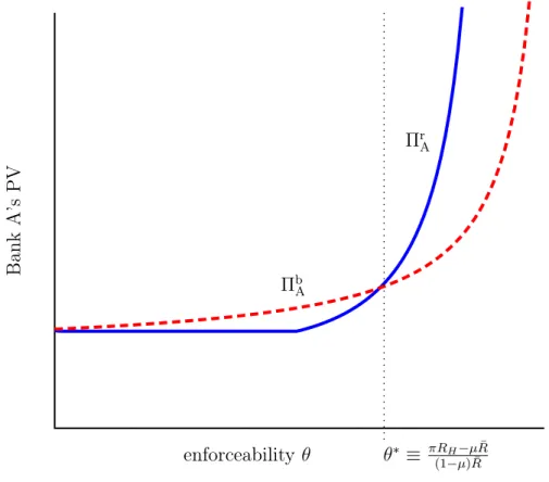
This section presents our main theoretical result that increasing enforceability θ leads Bank A to favor repos and thereby leads to credit chains—Bank C lends to Bank B, which lends to Bank A.
To determine when Bank A borrows via bonds and when it borrows via repos, we compare its PV in each case by comparing the expression for Πb
A in equation (3) with
the expression forΠrAin equation (7). This comparison is illustrated in Figure 8. Bank A borrows via bonds whenever ΠbA≥ΠrA or
(1−θ)eR¯
1−πθRH
≥ (1−θ)eR¯
1−θ µ+ (1−µ)θ¯ R, which can be written as
πRH ≥ µ+ (1−µ)θR.¯
With the above equation, we have derived that increased enforceability leads Bank A to prefer repos. We now state this as Proposition 3.3.1.
Proposition 3.3.1. Bank A borrows via bonds only if
θ≤θ∗ := πRH−µR¯ (1−µ) ¯R and borrows via repos otherwise.
This result is the key result behind our main finding that increasing enforceability can increase systemic risk, since more enforceability leads banks to rely more on non-resaleable instruments—on repos—and borrowing via non-non-resaleable instruments leads to credit chains.
3.4 Implications for Systemic Risk
In this section we analyze the effect of increasing enforceability on risk in the financial system as a whole. Here, we analyze when risk on the balance sheet of a single institu-tion can spread beyond that instituinstitu-tion’s immediate creditors, in particular, when one bank’s default causes the default of other banks. This is our notion of systemic risk, which we call a default cascade and restate in the next definition.
Definition3.4.1. A default cascade is an event in which a bank fails as a consequence of another bank’s failure. In the model, this occurs whenever Bank B fails (which occurs only because its debtor, Bank A, has failed).
Bank A’s PV from Issuing Bonds and Repos as a Function of Enforceability B an k A ’s P V enforceability θ θ∗ ≡ πRH−µR¯ (1−µ) ¯R Πr A Πb A
Figure 8: When enforceability is low (θ≤θ∗) Bank A’s PV is higher from issuing bonds; when
enforceability is high (θ > θ∗) Bank A’s PV is higher from issuing repos. The parameters
Bank B can fail only when it has debt to default on. Bank B has debt only when it borrows from Bank C to satisfy its liquidity needs. This occurs only when Bank A borrows via repos. In this case, since repos are not resaleable, Bank B cannot find liquidity by selling Bank A’s debt in the market; as a result, Bank B borrows from Bank C creating a credit chain. Hence, Bank A’s default can lead to Bank B’s default—i.e. default cascades can occur only when Bank A borrows via repos. The next result is that default cascades only happen when enforceability is high. This follows as a corollary of Proposition 3.3.1.
Corollary 3.4.1. Default cascades occur only when enforceability is high, specifically when
θ > θ∗ ≡ πRH −µR¯
(1−µ) ¯R .
This result says that increasing enforceability increases systemic risk in the sense that increasing enforceability can cause default cascades. Specifically, with repo bor-rowing, a credit chain emerges in which Bank A borrows from Bank B and Bank B borrows from Bank C. When Bank A’s project fails it defaults on its debt to Bank B. This depletes the left-hand side of Bank B’s balance sheet, so Bank B cannot cover its debt to Bank C and Bank B also defaults.
4
Generalizations, Extensions, and Robustness
In this section, we extend the analysis in seven ways. First, we explicitly incorporate securities as collateral into our model. Second, we consider a more general version of our model and argue that our results may hold in many debt markets, not only the interbank market. Third, we consider the possibility that Bank A borrows via one-period debt and rolls over at Date 1. Fourth, we allow for credit chains with more than two links. Fifth, we consider the effects of a short-term stay for repos, rather than an all-out exemption. Sixth, we consider the effects of a tax on repo borrowing. Finally, we consider implications for social welfare, not just systemic risk. Our results are robust to all these extensions.
4.1 The Role of Collateral
Repos and asset-backed commercial paper are collateralized by financial securities. In our model, we have assumed that Bank A’s project serves as collateral for its debt. In this section, we argue that our main results are robust to the use of securities as collateral. We do this in two ways. (i) We argue that Bank A’s project may be
interpreted as an investment in financial securities, where Bank A borrows from Bank B to buy the securities on margin. With this interpretation, our model captures the use of securities as collateral as-is. (ii) We modify the model so that Bank A pledges liquid securities to fund an illiquid project and show that our results are robust. We also discuss both economic and institutional reasons that Bank A may prefer to raise capital by using its securities as collateral rather than selling them in the market.
Investment as buying on margin. So far, we have viewed Bank A’s project as an investment in a real technology. However, given that it has constant returns to scale, we can also view it as a financial investment in securities. With this interpretation, Bank A wishes to invest in securities because it believes they are undervalued, i.e. Bank A has the view that the securities will generate high returns and is willing to pay interest to Bank B to borrow and invest in them. Specifically, Bank A borrows I from Bank B and investse+I in the securities, pledging the securities as collateral to Bank B. This corresponds to Bank A buying the securities “on margin” from Bank B, where Bank A’s endowmente serves as the “haircut.” Given this interpretation, our model already captures the use of securities as collateral in interbank markets. However, below we explore another interpretation, in which Bank A uses financial securities as collateral to borrow and invest in a real technology.
Collateralizing other securities. Consider the following twist on the baseline model which gives a role for securities to be used as collateral. In addition to its en-dowment and its project, Bank A holds securities that have Date-2 payoffs˜∈ {sL, sH},
where sL < sH. Denote the probability that s˜ = sH by p := P{s˜=sH} and the
expected value of the securities by s¯:= psH + (1−p)sL. Here, we assume that only
securities are pledgeable. Specifically, enforceability is zero for the cash flows that Bank A gets from its project andθ for securities.20 Thus, Bank A must use its securities as collateral in order to borrow and invest in its project. We assume thatsLis low enough
that Bank A prefers to lever up and default ifs˜=sL(this is the analogy of Assumption
2.5.3, which states that RL is low). This assumption may seem not to apply to “safe”
collateral such as government bonds. However, the results in this section hold even if the probability 1−p that the securities decline in value is very small, and realistically even safe securities may lose value quickly with some probability. Finally, we assume that, as in the baseline model, bond creditors recover nothing in bankruptcy, whereas repo creditors still recover the proportionθ of the collateral, where here the collateral constitutes the securitiess˜.
20
The idea that assets are pledgeable but cash flows are not is common in the literature. See, for example, Hart and Moore (1998) or Tirole’s (2006) textbook, which suggests that “collateral pledging makes up for a lack of pledgeable cash...borrowers must borrow against assets” (p. 169).
Consider first the case in which Bank A borrows via bonds. Given that the securities
˜
sare serving as collateral, these bonds can represent asset-backed commercial paper or short-term covered bonds. In this case, we can write Bank A’s borrowing constraint analogously to equation (2): due to the bankruptcy costs associated with bonds, the amount that Bank B is willing to lend to Bank A is limited by a proportion θ of its repayment in the event thats˜=sH,21
Ib,coll.≤pθsH.
This constraint binds at the optimum and Bank A’s PV is
ΠbA,coll.= e+Ib,coll.¯
R+ (1−θ)¯s
= (e+pθsH) ¯R+ (1−θ)¯s.
(9)
Now turn to the case in which Bank A borrows via repos. In this case, we can write Banks A’s borrowing constraint analogously to equation (6): because repos are not resaleable, the amount that Bank B is willing to lend takes into account the fact that Bank B may have to borrow against Bank A’s repo in the event that Bank B suffers a liquidity shock,
IAr,coll.≤µθs¯+ (1−µ)θ2¯s
=θ µ+ (1−µ)θ
¯
s. This constraint binds at the optimum and Bank A’s PV is
ΠrA,coll.= e+Ir,coll.¯ R+ (1−θ)¯s = e+θ µ+ (1−µ)θ ¯ s¯ R+ (1−θ)¯s. (10) Comparing this expression withΠbA,coll. gives the next proposition, which confirms that the main results of the model are robust to the case in which securities must be used as collateral.
Proposition4.1.1. Bank A borrows via bonds only if enforceabilityθis below a thresh-old, i.e. ifθ≤θs where
θs= psH −µs¯ (1−µ)¯s.
Thus, credit chains emerge and default cascades can occur for only high levels of en-forceability.
21
Note that since the project’s cash flows are not pledgeable, the amount that Bank A repays is independent of the realization of its returnR˜.
Proof. See Appendix A.3.
Reasons to use securities as collateral rather than sell them. In the analysis above we have assumed that Bank A used it securities ˜sas collateral to raise capital. We did not consider the possibility that Bank A sell its securities in the market at Date 0 and invest the proceeds in its project, thereby avoiding the frictions in the credit market. This assumption may be justified if there are institutional arrangements that prevent Bank A from liquidating its securities even when it is efficient. For example, it may hold securities on behalf of clients that it is not free to sell but is still allowed to use as collateral. Alternatively, it may need to hold the securities for regulatory reasons, for example to meet liquidity or capital requirements. However, Bank A may also prefer to hold its securities to maturity rather than to liquidate them because it places a higher value on the securities than it can obtain in the market, as we now describe.
Suppose that Bank A believes that its securities are more valuable than Bank B and Bank C believe they are. Specifically, suppose that Bank A believes that the probability that s˜= sH is p+ ∆p, whereas Bank B and Bank C believe this probability is p, as
above. Formally,∆p >0captures Bank A’s relative optimism, but it could also stand
in for other benefits that Bank A receives from holding the securitiess˜. For example, if the securities are shares, then Bank A may have private benefits of control from holding them. Alternatively, the securities could be useful for risk management, hedging against risks that Bank A holds elsewhere in its portfolio.
We now solve for a sufficient condition for Bank A to prefer to use its securities as collateral rather than to sell them in the market. If Bank A sells its securities to invest in its project, it raises their fair value ¯s≡psH + (1−p)sL in capital, so its PV is
Πsell coll.A = (e+ ¯s) ¯R. (11)
We now compare this to Bank A’s PV if it issues bondsunder its own beliefs. Modifying equation (9) to account for Bank A’s optimistic beliefs gives
ΠbA,optimistic= e+Ib,coll.¯ R+ (1−θ) (p+ ∆p)sH+ (1−p−∆p)sL = e+Ib,coll.¯ R+ (1−θ) ¯s+ (sH −sL)∆p . (12)
If this expression is greater than the payoff Πsell coll.A from selling securities, then Bank A always prefers to use its securities as collateral rather than liquidate in the market.22
22
Whereas this condition implies Bank A prefers to borrow via bonds than to sell its securities, it is not a sufficient condition for it to borrow via bonds. It may still prefer to borrow via repos.
The next proposition gives a condition under which Bank A will always use its securities as collateral rather than selling them in the market.
Proposition 4.1.2. Bank A uses collateral as long as its optimism ∆p is above a threshold, i.e. if∆p ≥∆∗p, where
∆∗p := (¯s−θpsH) ¯R−(1−θ)¯s (1−θ)(sH −sL)
. Proof. See Appendix A.4.
4.2 More General Instruments
So far, we have focused on the trade-off between borrowing via bonds (commercial paper) and repos in the interbank market. In this section, we argue that our main result—that increasing enforceability leads to credit chains and, therefore, increases systemic risk—generalizes to other markets. In fact, the basic mechanism may be at work in nearly all debt markets, even absent the formal, legal differences in resaleability and bankruptcy seniority that exist between repos and bonds. The reason is as follows. In addition to legal non-resaleability, fundamental economic frictions such as adverse selection can inhibit the resaleability of debt.23 A debt issuer may mitigate these frictions at a cost—for example by using securitization to combat the lemons problem— and thereby make debt resaleable or “liquid” in secondary markets. When enforceability increases, however, the relative benefits of resaleability decrease and, as a result, issuers are not willing to pay the cost to issue resaleable debt. Thus, for high enforceability, creditors, unable to sell their assets, may enter into new debt contracts to meet liquidity needs. This is the creation of a credit chain, which harbors systemic risk, just as in our baseline analysis. We formalize this argument below. The analysis in this section does not depend on (i) the assumption that bankruptcy is costly or (ii) the assumption that the outcome R of Bank A’s project is non-contractable. We make these assumptions above only for realism of the application to interbank loan markets.
Here we abstract from legal asymmetries. Rather, we follow Kiyotaki and Moore (2005) and assume that adverse selection frictions inhibit the resale of debt in the secondary market, but that an issuer can pay an upfront cost to mitigate these fric-tions.24 Specifically, we modify the model above in the following way. When Bank A
23
See Kiyotaki and Moore (2002) for a list of reasons that “between the date of issue and the date of delivery, an initial creditor C may not be able to resell [the debtor] D’s paper on to a third party...insofar as D gets locked in with C ex post.” (p. 62)
24
See page 703 of Kiyotaki and Moore (2005) for a discussion of this adverse-selection-based microfoun-dation. Kiyotaki and Moore (2000, 2001a, 2005, 2012) make similar assumptions.
borrows from Bank B, it can pay a proportional cost c to securitize its project. That is, if Bank A securitizes its project, its returns are decreased by the proportion c to
(1 −c)R, R ∈ {RL, RH}. Securitization circumvents the adverse selection friction,
making Bank A’s debt resaleable. There are no bankruptcy costs. We now analyze when Bank A will choose to securitize its project, forfeiting some returns but making its debt liquid/resaleable.
Consider first the case in which Bank A doesnotsecuritize its project. Here its PV is simply the repo PV expression in equation (8):
Πno sec.A = max ( eR,¯ (1−θ)eR¯ 1−θ µ+ (1−µ)θ¯ R ) .
Now turn to the case in which Bank A securitizes its project. Securitization lowers the returns on its project, but eliminates the cost associated with the liquidity shock. This observation allows us to write Bank A’s PV in this no-securitization case immediately. We simply scale down the returns by a factor1−cand replace the probability 1−µof a liquidity shock with zero:
Πsec.A = max e(1−c) ¯R,(1−θ)e(1−c) ¯R 1−θ(1−c) ¯R . Now, Bank A securitizes only when Πsec.
A ≥ Πno sec.A . This inequality leads to the
main result of this section, that Bank A securitizes only below a threshold level of enforceabilityθ∗∗. Thus, credit chains emerge only for high levels of enforceability and,
therefore, increasing enforceability increases systemic risk as in Subsection 3.4 above. We summarize this in Proposition 4.2.1 below.
Proposition4.2.1. Bank A securitizes its debt only if enforceabilityθis below a thresh-old, i.e. ifθ≤θ∗∗ where
θ∗∗:= 1 2 −1 + s 1 + 4c (1−µ)(1−c) ¯R ! .
Thus, credit chains emerge and default cascades can occur for only high levels of en-forceability.
Proof. See Appendix A.5.
This result demonstrates that our finding that increasing enforceability can increase systemic risk is not specific to the interbank market. Rather, the interbank market is just an environment in which systemic risk arising from credit chains is especially