NBER WORKING PAPER SERIES
THE IMPACT ON CONSUMPTION AND
SAVING OF CURRENT AND FUTURE FISCAL POLICIES Katherine Grace Carman
Jagadeesh Gokhale Laurence J. Kotlikoff Working Paper10085
http://www.nber.org/papers/w10085
NATIONAL BUREAU OF ECONOMIC RESEARCH 1050 Massachusetts Avenue
Cambridge, MA 02138 November 2003
Section 3 of this study draws heavily from Bernheim, Carman, Gokhale, and Kotlikoff (forthcoming 2003). The views expressed herein are those of the authors and not necessarily those of the National Bureau of Economic Research.
©2003 by Katherine Grace Carman, Jagadeesh Gokhale, and Laurence J. Kotlikoff. All rights reserved. Short sections of text, not to exceed two paragraphs, may be quoted without explicit permission provided that full credit, including © notice, is given to the source.
The Impact on Consumption and Saving of Current and Future Fiscal Policies Katherine Grace Carman, Jagadeesh Gokhale, and Laurence J. Kotlikoff NBER Working Paper No. 10084
November 2003 JEL No. H2, E6
ABSTRACT
This paper uses ESPlannerTM -- a life-cycle, financial planning model -- to investigate the potential
impact of alternative fiscal policies on current consumption and saving. Studies to date have examined the response of current consumption to tax-induced temporary and permanent income changes. To our knowledge, however, no study has directly examined whether consumption smoothing is actually feasible. ESPlanner’s saving and life insurance recommendations generate the smoothest possible survival-state contingent lifetime consumption path for the household without putting it into debt. Such consumption smoothing is predicted by economic theory and appears to accord closely, on average, with actual behavior. By running households through ESPlanner based on current policy as well as on alternative fiscal policies, one can easily compare the program's consumption response to hypothetical tax and transfer policy changes and assess the degree to which borrowing constraints may be playing a role in determining the size of those responses.
The households used in our analysis are drawn from the Federal Reserve's 1995 Survey of Consumer Finances. This data set provides detailed information on household earnings, assets, housing, demographics, and retirement plans -- all of which is used by ESPlanner in formulating its recommendations. The policies we consider are tax hikes, tax cuts, social security benefit cuts, and the elimination of tax-deferred saving. Our analysis distinguishes between immediate and future policy changes as well as between permanent and temporary ones.
Our results are influenced by the fact that a majority—57 percent—of our sample of households, many of which are young, is borrowing-constrained and, thus, more responsive to current than future policy changes no matter how long their duration. The results are also very sensitive to the particular policy being enacted. Income tax changes, for example, have little effect on the consumption/saving of low-income households for the simple reason their income tax liabilities are relatively small. And social security benefit cuts will have minor effects on the young because they lie so far in the future and the young are generally borrowing constrained. On the other hand, eliminating tax-deferred saving will have no effect on current retirees, but greatly influence the spending of the young, since such a policy would relax their borrowing constraints.
The significant heterogeneity in consumption/saving responses to policy changes depending on the ages and resource levels of the households in question and the particular policy undertaken makes it difficult to summarize our quantitative findings apart from saying that each of the policies considered has a quite sizeable impact on the current consumption and saving behavior of a substantial subset of our sample.
Katherine Grace Carman Stanford University Jagadeesh Gokhale
The Federal Reserve Bank of Cleveland The American Enterprise Institute
Laurence J. Kotlikoff Department of Economics
Boston University, 270 Bay State Road Boston, MA 02215
and NBER [email protected]
1. Introduction
How does household consumption and saving respond to changes in taxes and government transfer payments? This is a particularly important question for policymakers since
they routinely change fiscal policy in order to either stimulate or grow the economy. According
to standard policy parlance, stimulating the economy means getting households to spend more
and save less, particularly in the short term. In contrast, growing the economy means getting the
household sector to consume less and save more, again primarily in the short term.
The notion that short-term changes in household consumption and saving will alter not just the mix of aggregate output, but also the overall level of output and employment, is, of course, a Keynesian view of the macroeconomy. It’s also one that’s deeply imbedded, it seems, in the economic mentalities of our nation’s politicians. Indeed, President Nixon famously declared “We’re all Keynesians” in discussing his own approach to fiscal affairs. Interestingly, he made this statement at precisely the moment that Keynesian economics was coming under its greatest attack from the Rational Expectations school.
Certainly, the postwar period is replete with examples of “stimulative” tax cuts. The most famous of these include those of President Kennedy, President Reagan, and current President Bush. Former President Bush and former President Clinton, on the other hand, raised taxes when the economy was performing well with the argument that doing so was important to long-run fiscal stability, capital formation, and economic performance.
The fact that politicians are frequently trying to either jumpstart consumption or encourage saving has promoted many economists to study the consumption response to fiscal policy changes. The literature here includes analyses of the permanent tax reductions enacted in 1964, 1981, and 1986, the temporary income surtax passed in 1968, and the tax rebates of 1975
and 2001. Most studies report that immediate tax cuts stimulate consumption, although the extent of that stimulus is generally measured with little precision.
Examples here include include Modigliani and Steindel (1977), Blinder (1981), Blinder and Deaton (1985), and Poterba (1988) all of which consider the consumption effects of either the 1968 or the 1975 tax changes or both. Another example is Wilcox (1989), who finds that permanent increases in Social Security transfers between the 1960s and 1980s impacted personal consumption spending positively. Shapiro and Slemrod (2003) use special surveys conducted during and after the 2001 tax rebate checks were mailed out and find no significant uptick in consumption. It is notable, however, that tax law changes in 2001 included a generous non-refundable credit against contributions by low and moderate income households to tax-deferred saving plans.
In contrast to the goodly number of studies that consider immediate policy changes, there are relatively few studies that consider the current consumption response to announcements of impending tax-law changes, whether temporary or permanent. Poterba (1988) is an exception. He reports no significant consumption response to anticipated future tax changes.
Taken as a whole, the literature can be read as indicating that fiscal policies matter to consumption, but that the consumption response is driven, in large part, by the prevalence of borrowing constraints. The importance for consumption of such constraints is noted in Browning and Lusardi (1996) and Mankiw (2000), and empirically supported by McCarthy (1995) and Parker (1999a). Our current study certainly confirms the importance of borrowing
constraints. We find that such constraints bind for a significant fraction of our households and
are a key factor in the current consumption response to policy changes.1
Notwithstanding lots of careful estimation, the empirical literature provides little means of knowing precisely how a particular household’s spending will respond to any given policy change. This state of play is not all that surprising given the very significant obstacles in conducting research on the response of consumption to policy changes. First, the fiscal policies that have been enacted over the years to improve short- or long-run economic performance have varied enormously. For example, the 2001 Bush tax cut featured reductions in tax rates and an increase in the child-tax credit, whereas the 2003 tax cut featured a reduction in the tax rate applied to dividends. Second, the response of current consumption and saving to fiscal policy should, according to theory, depend very sensitively on the type and duration of the policy. Third, one needs to specify an explicit model of household intertemporal consumption choice to have any hope of properly assessing policy responses. This means structural estimation, which is more heroic and also less persuasive. And fourth, understanding how any particular household’s consumption should respond to any particular policy change requires detailed information about that household’s current and future expected resources, its housing and other “off-the-top” spending, and its current and likely future demographic composition.
One might think that the Congressional Budget Office or the Joint Committee on Taxation would have, by this point, developed theoretically sensible and carefully calibrated micro simulation models to score the revenue and spending effects of actual and proposed
1 Souleles [1999 and forthcoming] and Parker (1999b) provide dissenting results. The find a large contemporaneous consumption response to the Reagan tax cuts and claim that borrowing constraints do not drive their results. However, they have been criticized for excluding or inadequately including low-income households who are more likely subject to borrowing constraints.
policies. But such work lies in the future. At the present time, both agencies utilize highly stylized and aggregated frameworks to examine the response of the household sector to policy changes. These frameworks focus on general equilibrium feedback effects, which, while important, occur over very long horizons.
The current paper provides what we believe is a first pass at the kind of model that might be used by these agencies to understand the first-order effects of policy changes on current
consumption and saving. To be precise, the paper uses ESPlannerTM -- a life-cycle, financial
planning model -- to study how alternative hypothetical fiscal policies might change current consumption and saving among American households.
ESPlanner recommends consumption and saving levels that smooth a household's living standard to the maximum extent possible without putting it into debt. Such consumption smoothing is predicted by economic theory and appears, on average, to accord closely with
actual behavior. By running households through ESPlanner based on current policy as well as
based on an alternative fiscal policy, one can easily compare the program's consumption and saving recommendations and assess the potential effect of the policy on those variables.
Our sample consists of 959 married households drawn from the Federal Reserve's 1995 Survey of Consumer Finances. This data set provides detailed information on household earnings, assets, housing, demographics, and retirement plans -- all of which is used by
ESPlanner in formulating its recommendations. The policies we consider are tax hikes, tax cuts, social security benefit cuts, and the elimination of tax-deferred saving. Our analysis distinguishes between immediate and future policy changes as well as between permanent and temporary ones.
When it comes to examining the impact of eliminating tax-deferred saving, we set up the experiment such that each household’s pre-tax labor compensation is the same whether or not we rule out tax-deferred saving. In the case that we rule it out, we increase worker’s pre-tax labor earnings by the amount the employer would otherwise have contributed to his/her retirement accounts.
Our results are influenced by the fact that a majority of our sample of households—57 percent—many of which are young, is borrowing-constrained and, thus, more responsive to current than future policy changes no matter how long their duration. As may be expected, very young households, especially those that are rich in terms of their present value of consumption are borrowing constrained. This is not surprising because most wealth for such households consists of human capital. For middle-income households, however, only the poorest have a high incidence of binding borrowing constraints. Finally, a relatively small fraction of households with household-heads already retired or close to retiring is borrowing constrained.
The results are also very sensitive to the particular policy being enacted. Income tax changes, for example, have little effect on the consumption/saving of low-income households for the simple reason their income tax liabilities are relatively small. And social security benefit cuts will have minor effects on the young because they lie so far in the future and the young are generally borrowing constrained. On the other hand, eliminating tax-deferred saving will have no effect on current retirees, but greatly influence the spending of the young, since such a policy would relax their borrowing constraints.
The significant heterogeneity in consumption/saving responses to policy changes depending on the ages and resource levels of the households in question and the particular policy undertaken makes it difficult to summarize our quantitative findings apart from saying that each
of the policies considered has a quite sizeable impact on the current consumption and saving behavior of a substantial subset of our sample.
Our paper is organized as follows. The next section describes ESPlanner and discusses its strengths and weaknesses with respect to understanding consumption and saving responses to policy changes. Section 3 introduces the data set, explains our sample selection criteria, and details our data imputations. Section 4 presents results, and section 5 concludes with recommendations for future research.
2. ESPlanner
ESPlanner uses dynamic programming to smooth a household’s living standard over its life cycle to the extent possible without allowing the household to go into debt. In making its
calculations, ESPlanner takes into account the non-fungible nature of housing, bequest plans,
economies of shared living, the presence of children under age 19, and the desire of households to make “off-the-top” expenditures on college tuition, weddings, and other special expenses. In
addition, ESPlanner simultaneously calculates the amounts of life insurance needed at each age
by each spouse to guarantee that potential survivors suffer no decline in their living standards compared with what would otherwise be the case.
ESPlanner’s calculates time-paths of consumption expenditure, taxable saving, and term life insurance holdings in constant (2001) dollars. Consumption in this context is everything the household gets to spend after paying for its “off-the-top” expenditures – its housing expenses, special expenditures, life insurance premiums, special bequests, taxes, and net contributions to tax-favored accounts. Given the household’s demographic information, preferences, and
living standard over time, leaving the household with zero terminal assets apart from the equity in homes that the user has chosen to not sell.
The amount of recommended consumption expenditures needed to achieve a given living standard varies from year to year in response to changes in the household’s composition. It also rises when the household moves from a situation of being borrowing constrained to one of being unconstrained. Finally, recommended household consumption will change over time if users intentionally specify that they want their living standard to change.
ESPlanner’s algorithm is complicated. But it’s easy to check ESPlanner’s reports to see that, given the inputs, preferences, and borrowing constraints, the program is recommending the highest and smoothest possible living standard that the household can sustain over time without going into debt. Checking here refers to seeing that the household’s terminal net worth is zero, that its net worth is never negative (or never falls below minus the specified positive borrowing limit), that the level of adult-equivalent consumption is either constant through time or rises as borrowing constraints become relaxed, and that survivors can afford the same living standard as they would have enjoyed had neither spouse died prior to reach his and her maximum ages of life.
Since the taxes paid by households depend on their total incomes, which include asset income, how much a household pays in taxes each year depends on how much it has consumed and saved in the past. But how much the household can consume and, therefore, how much it will save depends, in part, on how much it has to pay in taxes. Thus taxes depend on income and assets, which depend on taxes. This simultaneity means that the time-paths over the household’s
achieves this simultaneous and consistent solution not only with respect to consumption and
saving decisions, but also with respect to the purchase of life insurance.2
Because taxes and Social Security benefits make a critical difference to how much a household should consume, save, and insure, casual calculations of these variables is a
prescription for seriously misleading financial recommendations.3 As mentioned, ESPlanner has
highly detailed federal income tax, state income tax, Social Security’s payroll tax, and Social Security benefit calculators. The federal and state income-tax calculators determine whether the household should itemize its deductions, computes deductions and exemptions, deducts from taxable income contributions to tax-deferred retirement accounts, includes in taxable income withdrawals from such accounts as well as the taxable component of Social Security benefits, and calculates total tax liabilities after all applicable refundable and non refundable tax credits.
These calculations are made separately for each year that the couple is alive as well as for
each year a survivor may be alive. Moreover, ESPlanner’s survivor tax and benefit calculations
for surviving wives (husbands) are made separately for each possible date of death of the
husband (wife). I.e., ESPlanner considers separately each date the husband (wife) might die and
calculates the taxes and benefits a surviving wife (husband) would receive each year thereafter.
Solution Method
The dynamic programming used in ESPlanner differs from traditional dynamic
programming in several respects. First, the software, which was developed by the authors,
2 The program not only calculates the appropriate levels of life insurance at each age for each spouse when both are alive. Bit also determines how much life insurance each surviving spouse needs to purchase.
3 See Gokhale, Jagadeesh, Laurence J. Kotlikoff, and Mark Warshawsky, “Comparing the Economic and Conventional Approaches to Financial Planning,” in Laurence J. Kotlikoff, Essays on Saving, Bequests, Altruism, and Life-Cycle Planning, Chicago, Ill.: University of Chicago Press, NBER volume, 2001, 489-560.
features two dynamic programs – one that calculates consumption/saving decisions, subject to borrowing constraints, and one that calculates life insurance holdings. Second, each program passes data to the other; i.e., the output of one program represents the input to the other. Third, finding a solution for the interrelated consumption, saving, and insurance problems requires iterating between the two programs until a fixed point is achieved with the following property: the inputs to one program (call it A) lead to outputs of the other program (call it B), which when passed to program A, generate the same outputs as were initially inputted into program B. This Guass-Seidel solution of mutually interdependent dynamic programs is, we believe, unique in the
literature.4
The inputs and outputs referred to here are survivor-state contingent time paths of variables. These variables include survivor-state contingent taxes, which are updated within each iteration to reflect the latest updated “guess” of asset income in each survivor-state. Hence, when the program reaches a fixed point on the path of survivor-contingent state variables, it will have reached a fixed point as well on survivor-contingent taxes. Stated differently, when the program converges it converges on all variables, including taxes.
There are two other questions to pose about ESPlanner’s convergence algorithm. First,
does it always converge? Second, is the solution it finds unique? The answer to the first question is that we’ve now run the program on thousands of actual and hypothetical households and have encountered no problems of convergence.5 The answer to the second question is that while we
don’t have a formal proof of uniqueness, we’ve never encountered any problems of uniqueness.6
4 Indeed, Economic Security Planning, Inc. was awarded a patent by the U.S. Patent Office for its software, including its dynamic programming methodology.
5 This includes runs made by commercial purchasers of ESPlanner.
6 The potential for non-uniqueness arises from the endogeneity of taxes to consumption choices. If total taxes were highly sensitive to asset income, one could conceive of low levels of consumption when young leading to very high
The Use of ESPlanner for Describing Actual Behavior
An obvious question that one might pose at this juncture is whether ESPlanner, which
was designed for prescriptive purposes, is useful as a descriptive tool, specifically one that tells us how households might respond to fiscal policy changes. As described in Bernheim, Berstein, Gokhale, and Kotlikoff (2002), Bernheim, Carman, Gokhale, and Kotlikoff (2003), and
Bernheim, Forni, Gokhale, and Kotlikoff (2003), the correlation between ESPlanner’s
recommended saving and life insurance holdings and actual saving and life insurance holdings is very low.
On the other hand, the mistakes, if one accepts that term, that households appear to be making are not systematic. Not all households are buying too little or too much life insurance. Nor are all households either under- or oversaving. Indeed, median behavior seems to accord with median recommendations. Hence, if one is trying to understand how the typical household’s consumption and saving would respond to major fiscal changes, the changes in
ESPlanner’s recommended levels of those variables may be a reasonable starting point.
One should also bear in mind that ESPlanner’s recommendations are consistent with
maximization of the most commonly posited intertemporal preference structure, namely
isoelastic preferences. The one caveat here is that ESPlanner’s implicit isoelastic preference
structures assume that the intertemporal elasticity of substitution is very close to zero. Stated
differently, ESPlanner planners implicit preferences exhibit very high risk aversion (they
levels of taxes when old that would justify low levels of consumption when old as well. On the other hand, with such a super sensitive tax function, high levels of consumption when young would generate very low taxes when old and permit high consumption when old. Any proof of uniqueness would need to be presented on a case-by-case basis since the tax function is dependent on each household’s demographics, age-earnings profile, and other circumstances. But the same quite extreme requirement for non-uniqueness would apply in each case, namely that increasing the present value of consumption by a dollar by raising consumption by the same percentage in each survivor-contingent state leads to more than a one dollar reduction in the present value of taxes.
approach Leontief), which implies the equalization across time, to the extent permitted by
borrowing constraints, of consumption per equivalent adult.7
The strong desire to equalize living standards across periods means that policy changes have only income effects in the model. This may lead to an overstatement of the absolute size of consumption changes associated with fiscal policies that raise or lower intertemporal terms of trade. For example, tax cuts that lower the net price of consuming in the future relative to the present will engender an income effect that raises current consumption, but a substitution effect
that lowers current consumption. ESPlanner assumes there are no such substitution effects.
This choice was made for computational convenience and to make the results of
ESPlanner as easily understood as possible to general users. On the other hand, there is solid empirical evidence supporting this formulation. Hall (1991) reviews this evidence, arguing that the intertemporal elasticity of substitution with respect to consumption is very small, if not zero.
3. The Data, Sample Selection, and Imputations8
The 1995 wave of the SCF was fielded between June and December 1995. Over those six months, the Federal Reserve surveyed over 4000 households. Like previous waves of the
SCF, the 1995 wave over-sampled the wealthy.9 The data collected cover demographics,
income, wealth, debt and credit, pensions, attitudes about financial matters, the nature of various transactions with various types of financial institutions, housing, real estate, businesses, vehicles, health and life insurance, current and past employment, current social security benefits,
7 The program does include an age-specific standard of living index that allows users to change their living standard through time, but for purposes of this study we assume there is no desired change in living standard as the couple ages. The living standard index can be thought of as age-specific time preference factors multiplying each period’s isoelastic utility.
8 This section draws heavily on Bernheim, Carman, Gokhale, and Kotlikoff (forthcoming 2003). 9
inheritances, charitable contributions, education, and retirement plans. The architects of the SCF
data files imputed missing information, supplying five “implicates” for each household.10 We
use the first implicate.
Sample Selection
Our final sample consists of 959 couples. From the original observation count of 2874 married couples, we excluded couples for the following reasons: a) a spouse was self employed or owned and actively managed a business (59.4 percent of excluded observations); b) a spouse was temporarily unemployed or both spouses were students or temporarily laid off (7.9 percent); c) neither spouse had regular earnings as an employee (15.6 percent); d) labor earnings were defined in terms of a unit other than time worked, for example by the piece (0.5 percent); e) mortgage information was inconsistent (7.1 percent); f) property taxes were greater than 5 percent of the value of the home (1.3 percent); g) a spouse was over the age of 85 (1.3 percent); Household head was aged 24 or younger (3.3 percent) or h) the couple’s reported income and other economic resources were insufficient to support its reported fixed expenditures (3.7
percent).11
Data Imputations Non-Asset Income
Our calculations require data on each spouse’s past and future covered earnings as well as future total (covered and uncovered) earnings. We assume that all earnings are covered. For
10Kennickell (1991) provides a description of the imputation procedure. 11
respondents who were working at the survey date, we have 1995 self-reported labor earnings. In order to impute past and future earnings we use a model that assumes that the cross section age-earnings profile for fully employed workers remains constant through time. We allow real wages for all ages to grow over time, using the historic Social Security real wage growth for past years, and a 1 percent overall real wage growth factor for future years. In estimating past Social Security covered earnings, we assume that the first year of employment is the maximum of 1951
and the year the person was age 22.12 Households where one of the spouses was temporarily not
working, as opposed to out of the labor force, were dropped from our sample.
The SCF provides information on other kinds of non-asset income. We treat some of these income sources, such as Veteran’s Benefits, SSI, disability income, welfare, child support, and regular help from friends or relatives, as non-taxable. Except for Social Security disability income and child support, we assume these income streams continue, with full adjustments for inflation, until the respondent’s death. Social Security disability income is assumed to end at age 62, when the recipient becomes eligible for Social Security retirement benefits. We divide child support received by the number of children to obtain child support per child and assume it
is received until the child in question reaches 18.13 We treat other kinds of special receipts, such
as income from trust funds and royalties, as taxable. We assume they will be received for ten years beyond the survey date, and that the payments will be constant in nominal terms. Relatively few respondents receive these kinds of income flows, and the amounts are generally small relative to average earnings. We assume that SCF respondents retire at their stated
12 For workers who were under 22 in 1995, we assume that 1995 was their first year of employment. 13
The HRS reports only the sum of child support and spousal support. However, we confine our attention to couples, 98 percent of which are married. Since spousal support generally ends upon remarriage (and also declines somewhat on average when individuals become unmarried partners), we can safely assume that the entire reported amount is child support.
intended ages of retirement or age 70, whichever is smaller. For those who fail to say when they will retire, we use age 65.
Pension Plans, Retirement Accounts, and Social Security
The SCF provides information on nominal benefits currently received from defined benefit pension plans as well as expected nominal benefits for future pension recipients. We assume that all pensions are indexed to inflation and that a surviving spouse would receive 100 percent of the monthly benefit or lump-sum distribution. We further assume that employer-sponsored defined contribution plans and all private retirement accounts (IRAs and Keoghs) provide for tax-deductible contributions and tax-deferred accumulation. Contributions in all future years up to age 59 are set equal, in real terms, to contributions in the survey year. If total contributions are greater than the legal limits ($30,000 or 25% of income) contributions are truncated. The proportion given by the employer remains constant. Any contributions (by the employee or the employer) over the legal limit are included in employee non-deductible and tax-favored contributions.
The SCF contains information on IRA account balances, but not annual contributions. We impute contributions based on Tobit regressions from the Consumer Expenditure Survey. Contributions are calculated as a function of marital status, work status, age, earnings, and family size.
If an individual is already receiving Social Security benefits, we assume that benefits have already started. Otherwise, we impute the initial age of benefit receipt as follows. If the individual is still working, we assume that benefits will start at his or her projected retirement age (but not earlier than age 62). If the individual is retired, we use the reported start date for
those currently receiving benefits, for those not yet receiving benefits we assume benefits will start at age 62 for those currently under 62, and at the current age for those over 62. In all cases, the initial age of benefit receipt is between 62 and 70. For respondents currently receiving social security disability benefits, we assume that they switch to retirement benefits at age 62. Our calculations also require information on the age at which individuals begin to receive private pension benefits. For those not yet receiving benefits, we use the age at which the individual expects benefits to begin, as reported in the SCF.
Individuals with previous marriages lasting more than ten years and ending in divorce or
separation and individuals with previous marriages lasting more than nine months and ending in the spouse’s death are eligible to receive Social Security benefits based on the earnings history of their prior spouse. This presents us with a problem, since we do not have any information about prior spouses. We assume that all such individuals receive benefits based on either their own earnings history or that of their current spouse.
Housing
Our calculations require information on a variety of specific housing expenditures, including mortgages, home insurance premiums, property taxes, and other recurring expenses. Association fees, homeowner or condo/coop/townhouse association fees and rent on the site for households owning and living in mobile homes are added to home insurance premiums to form recurring house expenditures. When you own part of a farm, you are classified as a homeowner. The rent you pay is then also added to your insurance premium. While it does not contain information on homeowner insurance premiums, it does include the face amount of insurance. We imputed annual home insurance premiums by multiplying the face values by 0.0025.
If the mortgage payment (minus property taxes and insurance premium if respondent states these are included in their payments) is negative then the observation is dropped. If the annual property tax is greater than 5% of the home value the observation is dropped. With regards to mortgages, the SCF reports the balance remaining, the number of years remaining, the interest rate, and the payment. In order to ensure consistency, we imputed the balance remaining on the mortgage based on the years remaining and the interest rate and payment.
In some instances, rental payments reported in the sample include heat and electricity expenses; in such cases, respondents were not asked separately about these utility payments. We apportion the reported number into separate components by assuming that the ratio of rent to utilities is the same for these respondents as the average ratio computed from the Health and Retirement Study. If rent includes all utilities, rent is set to 0.77*rent. If rent includes some utilities, rent is set to 0.89*rent. We have no information on utility expenditure if it is not included in rent. The SCF does not include any information concerning property taxes paid on second homes. We assume that this property is taxed at the same rate as the primary home. Finally, we set monthly rental payments equal to zero for the few respondents who report that they live in a house or apartment that they neither rent nor own. In addition, we assume that all households plan to remain in the same house before and after retirement.
Other Variables
For confidentiality reasons, the SCF does not report the respondent’s date or month of birth or state of residency. We assume that each respondent was born on the fifteenth of June. For the purposes of computing state taxes, we use Massachusetts law. We set the maximum age
of life to 95 for all individuals. Many households have adult children living with them. For the purposes of this project, only children 18 or under are included.
We assume for all respondents a fixed amount for funeral expenses which is set equal to the median of the reported expenses ($5000) for HRS spouses for spouses actually died in 1991 (90 observations). The HRS reports information on actual funeral expenses and legal fees of deceased spouses. We set intended bequests equal to zero.
The SCF allows mortgages to end with a balloon payment. When there is a balloon payment, we assume that they refinance for the amount of the balloon payment with a 15-year mortgage (8% interest rate). There is no space in ESP for future mortgages so these are included in special expenditures. Interest payments on the first home are included in deductible special expenditures. Payments on the balance are included in non-deductible special expenditures. Non-deductible special expenditures also include child support or alimony payment and support to other family members. These are assumed to be paid in the current year and the next four years (a total of 5 years). Non-deductible special expenditures also include child support or alimony payment and support to other family members. These are assumed to be paid in the current year and the next four years (a total of 5 years).
As a measure of a household’s net worth, we use total non-housing assets minus total non-housing liabilities. Total non-housing assets include checking and saving accounts, money market funds, CDs, government saving bonds, T-bills, stocks, mutual funds, investment trusts, business equity, bonds, bond funds, real estate other than primary and vacation homes, the cash value of life insurance policies, and some miscellaneous items. Total non-housing liabilities include personal loans, student loans, credit card balances, car loans, installment loans, and other non housing debt. Housing debt (mortgages and equity lines of credit) are considered separately
(see above). We assume that, apart from mortgages and other outstanding housing debt, households cannot borrow against future income. We further assume a 3 percent rate of inflation and a 3 percent real pre-tax rate of return. Finally, we set our couples’ borrowing limits to zero
and tell ESPlanner to maintain a constant living standard over time for all household members,
regardless of the survivorship states, provided this does not violate the household’s no debt constraint.
4. Findings
Table 1 indicates the number of final sample observations after all sample selection criteria have been applied. These counts as well as other results are cross-classified by the age of the household head and the present value of remaining lifetime consumption expenditure. Consumption is defined here and elsewhere to include housing consumption. In the case of couples that rent, housing consumption is measured as annual rental payments and non-rental expenses. In the case of couples that own their own homes, housing consumption is measured as the sum of imputed rent plus homeowner’s insurance, property taxes, and maintenance expenses. Imputed rent, in turn, is measured as 6 percent of the value of the home reflecting an assumed 3 percent real return on comparable safe investments and a 3 percent annual depreciation rate.
The present value of consumption refers to the actuarial present value of what the couple
can expect to consume given the chances that one or both spouses will die prior to her or his maximum age of life. To form these present values we apply survivor state-specific survival probabilities to consumption in each survivor state, where a survivor state is defined not only by the year and age of the survivor, but also by the age at which the spouse died. Hence, the present
value of consumption is a comprehensive measure of the couples expected remaining lifetime resources.
Returning to the table, note that of our 959 observations, most have lifetime consumption values ranging from $500,000 to $2 million. Thanks to the survey’s over-sampling of the wealthy, there are 59 households with present values of consumption in excess of $4 million. The majority of the sample – 78 percent -- is under age 55. Those age 65 to 74 represent 7 percent of the sample.
Overall 57 percent of our sample of households is borrowing constrained. As Table 2 shows, a large fraction of young households tend to be borrowing constrained. For example, almost all of the households with the head aged in the 25-34 year range are borrowing constrained. The fraction of the youngest and lifetime-rich households that are borrowing constrained is not much lower: Even among those with present value of consumption in the $2-$4 million range, 80 percent are borrowing constrained. This is, of course, not surprising as most young households’ wealth is in the form of human capital the returns from which are mostly realized later. The same is not true of middle-aged households. Take households with heads aged in the 45-54 year range: More than 80 percent of those in the $0-$250 thousand present value of consumption range are borrowing constrained. However, of those in the $2-$4 million dollar present value of consumption range, only 30 percent are borrowing constrained. Again, low present value of consumption households in this age range may face significant out-of-pocket expenses on childrens’ education and housing. In addition, they may be planning to finance most of their retirement consumption out of Social Security benefits. As Gokhale, Kotlikoff and Warshawsky (forthcoming 2004) demonstrate, such households may have neither the ability nor need to accumulate significant savings by middle age. Nevertheless, their
projected earnings growth could permit a higher future consumption level—one that they cannot smooth because of their inability to borrow. Finally, a much smaller fraction of households with the oldest heads (aged 65-74) is borrowing constrained.
Table 3 shows the fraction of households that would continue to be borrowing constrained even if their DC pension contributions were eliminated (and any employer matching contributions were returned as higher wages). This change has little impact on the number of the youngest households that are borrowing constrained. For example, over 60 percent of households with heads aged 25-34 and present value of consumption in the range $1-$2 million remain borrowing constrained. Most of the impact is on poorer and relatively younger (but not the youngest) households. For example, only 40 percent of those households aged 35-44 with $250-$500 thousand in present value of consumption remain borrowing constrained after eliminating their DC pension contributions as opposed to more than 90 percent with such contributions. Clearly, many young and lifetime-poor households seem to be sacrificing current consumption in order to continue their contributions to DC pension plans.
Consumption Rates
Tables 4 through 6 provide a measure of ESPlanner’s recommended consumption and
saving behavior. The figure in these tables are consumption rates – defined as the ratio of
current consumption to the present value of lifetime consumption. These consumption rates can also be thought of as average propensities to consume out for remaining lifetime resources since the present expected value of consumption is quite close in value to the present value of remaining lifetime resources.
The idea in presenting these consumption rates is to show how fast ESPlanner
recommends that households expend their consumption power. This measure of consumption behavior is an alternative to current saving rate measures, which are highly sensitive to how one defines current income.
According to the life cycle model, we’d expect these consumption-spending rates to rise with age, which they certainly do in all three tables. Consider, in this regard, table 5, which shows median consumption rates. These rates almost double as one moves from ages 25-34 to 65-74. Also note that the poorest young and middle-aged households have lower consumption rates that those of the same age, but with higher levels of lifetime consumption. This reflects the fact that poor/young couples are more often borrowing constrained than are rich/older couples.
We can further explore the issues of borrowing constraints by comparing the minimum and maximum consumption rates presents in tables 4 and 6 with the median rates presented in table 5. Were borrowing constraints nonbinding and and were there no differences in the number and ages of children as well as the ages of spouses, we’d expect all consumption rates to be the same at a given age regardless of the household’s level of resources. But as a quick comparison of tables 4 and 5 indicate, minimum consumption rates are much lower and maximum rates are often considerably higher than the median rates.
The differences in minimum and maximum rates are striking, but not surprising. One would expect that if some households are borrowing constrained, the depression in their current consumption relative to that of non-borrowing constrained households would show up as a large difference between the maximum and minimum consumption rates. Table 7 shows this difference (maximum minus minimum consumption rate). For the poorest households, the difference generally exceeds 2 percentage points and declines gradually but unmistakably as the
present value of consumption rises—the difference is less than 2 percentage points for richer households, in general. Hence, the differential impact of binding liquidity constraints on consumption rates for poor versus rich households is evident despite the considerable sampling
variation in households’ economic and demographic circumstances.14
Tax Changes
Tables 8 through 13 show the median percentage change in consumption within each age-present value of consumption cell of various changes in income taxes. The first three of these tables consider across the board 30 percent tax cuts. Table 7 cuts taxes immediately and permanently. The pattern of responses is quite interesting. The richest households exhibit the largest responses. Indeed, for those who consume $4 million and more in present value, the consumption response ranges from 9.0 percent to 14.1 percent. For the middle-class, the consumption response is approximately 3 percent. And for the poor, the response is generally quite low. Intuitively, the rich pay the most in taxes and are the most responsive to the tax cuts. This is the opposite of the common view that tax cuts generate the largest consumption response
by the poor.15 The other interesting point of the table is that the largest consumption responses
arise among the young and middle-aged. The reason is that taxes are a bigger share of consumable economic resources for younger age groups than they are for the elderly. Stated differently, taken as a group, the elderly finance much of their consumption out of the principal on their assets, none of which is subject to income taxation.
14 The biggest differential occurs in the case of households whose heads are aged 45 through 54 and whose present value of consumption lies between $2 million to $4 million. This large difference is driven by one observation with a minimum consumption rate of 0.56 percent. The corresponding maximum rate of 5.2 percent does not seem anomalous when compared to the maximum rates for neighboring cells. The observation with the lowest consumption rate has a particulary strongly binding borrowing constraint that makes its current consumption extremely low relative to the present value of its consumption.
15 One might argue that our exclusion of intentional bequests on the part of the rich is biasing our results. But were we to include bequests, we’d expect to generate very similar findings provided preferences toward bequests and consumption were homothetic.
Table 9 repeats the experiment of table 8, but cuts taxes for only 5 years. The responses are dramatically smaller, particularly for the rich. For example, the richest 45-54 year-old households increase their consumption by 11.3 percent if taxes are cut permanently, but by only 2.7 percent if they are cut for only 5 years. This point is particularly salient given that recent federal income tax cuts are formally slated to be short lived. The smallest discrepancies between the table 8 and table 9 results arise for the young, a disproportionately high percentage of which is borrowing constrained. Were the entire sample borrowing constrained, one would expect to see little if any difference in the table 8 and table 9 results. The fact that the results do differ significantly indicates that borrowing constraints do not dictate the overall response of consumption to tax cuts.
Table 10 takes another cut at the income tax cut. In this case, the 30 percent tax cut is permanently applied, but only after a delay of 10 years. The consumption responses are generally much smaller than either the immediate permanent or the immediate temporary tax cuts. The exception is the rich for whom long-lasting future tax cuts deliver larger present value tax breaks than equal sized, immediate, but short-live tax cuts.
Tables 11 through 13 run the tax policy in reverse. Table 11 raises taxes immediately and permanently by 30 percent; table 12 raises taxes immediately but only for 5 years; and table
13 increases taxes permanently by 30 percent, but not before 10 years. As one would expect,
table 11’s results are very similar to those in table 8; i.e., whether taxes are raised or lowered by 30 percent, the immediate percentage consumption response, measured in absolute value, is quite similar. Similarly, table 12’s findings are quite close to those in table 9 and table 13’s findings are similar to those of table 10.
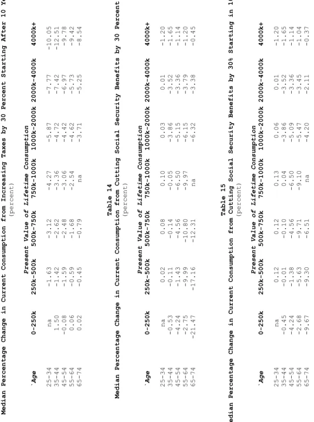
Cutting Social Security Benefits
Tables 14 and 15 consider, respectively, 30 percent permanent cuts in Social Security benefits starting either immediately or after ten years. As one would expect, the immediate cuts have major effects on the current consumption of the elderly, particularly the poor elderly. Indeed, the poorest elderly reduce their current consumption by more than one fifth. For the richest elderly, the benefit cut is negligible in terms of the change in consumption that it engenders. Another noteworthy aspect of these tables is that the consumption response of those aged 45-54 who are poor through moderately well off. They respond significantly even though their actual receipt of benefits is fairly far off in time.
Table 15 shows a very significant current consumption response to long-range benefit cuts. Those moderately well off and aged 55-64 reduce their current consumption by over 9 percent, which is very similar to their response if benefits are cut immediately since most of these cohorts must wait for several years before receiving annual benefits. The possibility that the response of current consumption to future benefit cuts could be sizable is probably well appreciated by policymakers and others and does not appear to influence discussions of Social Security and Medicare reform options.
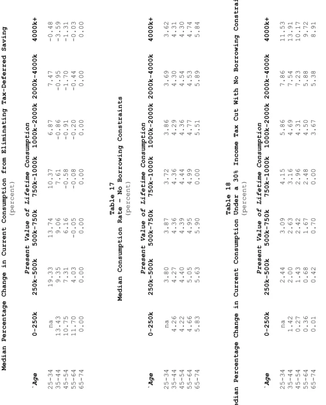
Eliminating Tax-Deferred Saving
Table, 16, shows the impact of eliminating, at the margin, 401(k) plans, traditional IRAs, Keogh plans, and other tax-deferred saving vehicles. As mentioned, our experiment here entails eliminating contributions to these plans, but maintaining pre-tax compensation unchanged by assuming that workers would receive higher salaries in lieu of their employers contributing to their plans.
The results show very large median consumption responses by the poor and, in general, the young. In the case of households age 25-34 with $250,000 to $500,000 in present value consumption spending, eliminating tax-deferred saving leads to a 19.3 percent rise in consumption. The primary explanation for this is the substantial relaxation of borrowing constraints associated with such a policy. But a second reason is that for some households, particular those with low incomes, participating in a 401(k) or similar tax-deferred account can raise, rather than lower, lifetime taxes. This effect, documented in Gokhale and Kotlikoff (2003), arises because significant withdrawals form tax-deferred accounts in retirement can trigger the taxation of Social Security benefits and also place the household in a higher tax bracket than would otherwise have been the case. On the other hand, Gokhale and Kotlikoff (2003) point out that the rich stand to save significantly on their lifetime taxes from participating in tax-deferred retirement plans. This explains why many of the entries in table 14 are negative – they reflect the reduction in consumption by those sample households who face higher lifetime taxes when tax-deferred retirement saving is shut down.
5. The Importance of Borrowing Constraints
Tables 17 and 18 repeat tables 5 and 8. Table 17 recalculates median consumption rates—the ratio of current consumption to the present value of lifetime consumption—in the absence of borrowing constraints. This is implemented by allowing the household to borrow as much as needed in order to be able to smooth consumption throughout its lifetime including survivors’ lifetimes. As expected, young households and those with low lifetime consumption would increase their consumption the most. For example, households aged 25-34 in the
$250,000 to $500,000 lifetime consumption range would increase their current consumption by almost a full percentage point (compare Table 17 with Table 5).
Finally, Table 18 shows the impact of the an immediate and permanent 30 percent tax cut when households face no binding borrowing constraints both without and with the tax cut. Two effects operate simultaneously in this experiment. First, when borrowing constraints are binding, (Table 8) households tend to consume immediately most or all of the additional after-tax income that the tax cut provides. When the borrowing constraint is nonbinding, households will smooth the gains from the tax cut over their entire lifetime. For older and poorer households, a relatively large portion of the gain occurs relatively early in the lifetime. Hence, the response of consumption to a permanent tax cut will, in general, be lower when the borrowing constraint is relaxed. A comparison of tables 8 and 18 shows this to be true for such households.
In contrast, the consumption response of younger and richer households is different: Because many of these households are borrowing constrained initially, table 8’s consumption response to the tax cut includes only the additional consumption such households can enjoy from the higher current after-tax income. The bulk of the tax reduction for such households, however, occurs later in their lifetimes that they are unable to smooth. Once the constraint is removed, these households’ consumption rises by more in response to a tax cut because they can bring forward the higher lifetime consumption made possible by the larger future increases in after-tax income. Note that the different impact on rich versus poorer households would not occur if the income tax system were proportional. Under our progressive income tax system, however, earnings growth pushes those who earn above a certain threshold into higher income tax brackets in future years, causing the tax saving from an across the board cut to be larger in future years. In each range of lifetime consumption greater than $500,000-$750,000, the consumption
response in Table 18 declines and approaches that of Table 8 as the age of the household increases. The explanation here is that older households’ prospective gains from the income tax cut are smaller.
5. Conclusion
This paper shows how a micro-based life-cycle model can assist economists and policymakers in understanding the short-term consumption and saving responses to immediate, projected, or temporary changes in fiscal policy. A large fraction of U.S. households—as much as 57 percent—appear to be borrowing constrained. Such constraints clearly play a major role in determining how many households respond, and by how much, to particular policies. Hence, these constraints should be included in any future analyses of conumer response to fiscal policy changes.
Clearly, having a larger sample and having more confidence that the model used is actually descriptive rather than simply prescriptive is very important. With a larger sample, one could extrapolate projected behavior to the overall population with more confidence. Checking the descriptive nature of the model boils down to fitting the model to the data. Doing so will require direct and comprehensive measures of consumption that are combined with detailed information on households’ past, current, and future economic resources. Unfortunately, no such data set currently exists. The best hope of procuring such a data set would be to administer the next Survey of Consumer Finances to respondents of the Consumer Expenditure Survey – something that seems may require substantial funding but may generate considerable insight into how households respond to alternative fiscal initiatives.
References
Bernheim, B. Douglas, Solange Berstein, Jagadeesh Gokhale, and Laurence J. Kotlikoff, “Saving and Life Insurance Holdings at Boston University,” mimeo May 2002.
Bernheim, B. Douglas, Katherine G. Carman, Jagadeesh Gokhale, and Laurence J. Kotlikoff, “Are Life Insurance Holdings Related to Financial Vulnerabilities?”
forthcoming, Economic Inquiry, 2003.
Bernheim, B. Douglas, Lorenzo Forni, Jagadeesh Gokhale, and Laurence J. Kotlikoff, “The Mismatch Between Life Insurance Holdings and Financial Vulnerabilities:
Evidence from the Health and Retirement Survey,” American Economic Review, 93 (1),
March 2003, pp. 354-65.
Blinder, Alan, S. “Temporary Income Taxes and Consumer Spending,” Journal of Political Economy, February, 1981, vol. 89, pp. 26-53.
Blinder, Alan, S. and Deaaton, Angus, “The Time Series Consumption Function Revisited,” Brooking Papers on Economic Activity, 2:1985, pp. 465-511.
Martin Browning and Annamaria Lusardi, “Household Savings: Micro Theories and Micro Facts,” Journal of Economic Literature, vol. 34, December 1996.
Gokhale, Jagadeesh and Laurence J. Kotlikoff, “Who Gets Paid to Save?” Tax Policy and
the Economy, NBER volume, MIT Press, 2003.
Gokhale, Jagadeesh, Laurence J. Kotlikoff, and Mark Warshawsky, “Life Cycle Saving,
Limits on Contributions on DC Pension Plans, and Lifetime Tax Benefits,” in Private
Pensions and Public Policies, ed. by William Gale, John Shoven, and Mark Warshawsky, Conference Volume, The Brookings Institution, forthcoming 2004.
Gravelle, Jane, G. “Tax Cuts and Economic Stimulus: How Effective are the
Alternatives?” CRS Report to Congress, Congressional Research Service, Apri, 2, 2002.
Hall, Robert E. “Substitution Over Time in Consumption and Work,” in L. McKenzie
and S. Zamagni (eds.), Value and Capital Fifty Years Later, MacMillan, 1991, pp.
239-267.
McCarthy, Jonathan, “Imperfect Insurance and Differing Propensities to Consume Across
Individuals,” Journal of Monetary Economics, Vol. 36, November, 1995, pp. 301-327.
Modigliani, Francom and Steindel, Charles, “Is a Tax Rebate an Effective Tool for Stabilization Policy?” Brookings Papers on Economic Activity, 1:1977, pp. 175-209.
N. Gregory Mankiw, “The Savers-Spenders Theory of Fiscal Policy,” American
Parker, Jonathan, A. “The Consumption Function Revisited” (working paper) Princeton University, August 1999a.
Parker, Jonathan, A. “The Reaction of Household Consumption to Predictable Changes in
Social Security Taxes,” American Economic Review, vol. 89, September 1999b, pp.
959-973.
Souleles, Nicholas, “The Response of Household Consumption to Income Tax Refunds,”
American Economic Review, vol. 89, September 1999, pp. 947-958.
Souleles, Nicholas, “Consumer Response to the Reagan Tax Cuts,” Journal of Public
Economics, (forthcoming).
Shapiro, Matthew, D., and Joel Slemrod, “Did the 2001 Tax Rebate Stimulate Spending?
Evidence from Taxpayer Surveys,” Tax Policy and the Economy, National Bureau of
Economic Research, vol. 17, 2003, pp. 83-110.
Poterba, James, M. “Are Consumers Forward Looking? Evidence from Fiscal
Experiments,” American Economic Review, Papers and Proceedings, Vol. 78, Number 2,
May 1988, pp. 413-18.
Wilcox, David, W., “Social Security Benefits, Consumption Expenditure, and the
31
Table 1
Number of Observations
Present Value of Lifetime Consumption
Age 0-250k 250k-500k 500k-750k 750k-1000k 1000k-2000k 2000k-4000k 4000k+ 25-34 0 15 28 30 133 20 3 35-44 5 25 52 35 121 23 10 45-54 5 24 41 33 84 40 21 55-64 6 24 21 16 48 13 14 65-74 7 15 12 1 14 9 11 Table 2
Number of Borrowing-Constrained Observations
Present Value of Lifetime Consumption
Age
0-250k 250k-500k 500k-750k 750k-1000k 1000k-2000k 2000k-4000k 4000k+
25-34 0 15 25 28 108 16 1 35-44 4 23 43 26 73 9 0 45-54 5 20 33 17 37 12 1 55-64 4 17 7 4 7 1 0 65-74 4 2 2 0 1 0 0
Table 3
Number of Borrowing-Constrained Observations in the Absence of Retirement Account Contributions
Present Value of Lifetime Consumption
Age
0-250k 250k-500k 500k-750k 750k-1000k 1000k-2000k 2000k-4000k 4000k+
32
Table 4
Minimum Consumption Rate
(percent)
Current Consumption / Present Value of Lifetime Consumption
Age
0-250k 250k-500k 500k-750k 750k-1000k 1000k-2000k 2000k-4000k 4000k+
25-34 na 1.53 1.63 1.61 1.68 2.47 3.28 35-44 2.40 2.99 1.54 2.87 2.89 3.50 3.65 45-54 2.57 2.35 2.79 2.16 3.44 0.56 3.95 55-64 2.58 2.39 3.34 4.17 2.44 4.11 4.36 65-74 4.56 3.29 5.10 na 5.01 4.94 4.88
Table 5
Median Consumption Rate
(percent)
Current Consumption / Present Value of Lifetime Consumption
Age
0-250k 250k-500k 500k-750k 750k-1000k 1000k-2000k 2000k-4000k 4000k+
25-34 na 2.91 3.01 2.67 3.29 3.28 3.62 35-44 3.33 3.67 3.89 3.83 4.07 4.27 4.31 45-54 3.85 3.97 4.06 4.19 4.19 4.38 4.26 55-64 3.95 4.69 4.81 4.95 4.76 4.53 4.74 65-74 5.82 5.55 5.90 na 5.46 5.89 5.84
Table 6
Maximum Consumption Rate
(percent)
Current Consumption / Present Value of Lifetime Consumption
Age
0-250k 250k-500k 500k-750k 750k-1000k 1000k-2000k 2000k-4000k 4000k+
33
Table 7
Percentage Point Different Between Maximum and Minimum Current Consumption Rate
(percent)
Current Consumption / Present Value of Lifetime Consumption
Age
0-250k 250k-500k 500k-750k 750k-1000k 1000k-2000k 2000k-4000k 4000k+
25-34 na 2.53 2.47 2.34 2.53 1.79 0.93 35-44 2.00 1.56 3.63 1.97 2.60 1.61 0.78 45-54 2.03 2.81 2.13 2.92 1.94 4.64 1.88 55-64 2.55 3.92 2.27 1.18 3.31 1.14 0.68 65-74 2.15 3.52 2.03 na 1.12 1.61 1.69
Table 8
Median Percentage Change in Current Consumption from Cutting Taxes by 30 Percent
(percent)
Present Value of Lifetime Consumption
`Age
0-250k 250k-500k 500k-750k 750k-1000k 1000k-2000k 2000k-4000k 4000k+
25-34 na 3.21 3.11 3.54 4.29 6.26 11.04 35-44 4.40 2.36 2.80 3.50 4.70 8.20 14.14 45-54 0.34 2.02 3.16 3.29 4.60 6.97 11.25 55-64 0.35 0.84 2.11 2.46 4.33 5.90 9.82 65-74 0.03 0.36 0.56 na 3.50 5.08 9.01
Table 9
Median Percentage Change in Current Consumption from Cutting Taxes by 30 Percent for Just 5 Years
(percent)
Present Value of Lifetime Consumption
`Age
0-250k 250k-500k 500k-750k 750k-1000k 1000k-2000k 2000k-4000k 4000k+
34
Table 10
Median Percentage Change in Current Consumption from Cutting Taxes by 30 Percent Starting After 10 Years
(percent)
Present Value of Lifetime Consumption
`Age
0-250k 250k-500k 500k-750k 750k-1000k 1000k-2000k 2000k-4000k 4000k+
25-34 na 0.09 0.08 0.05 -0.01 -0.06 3.41 35-44 1.17 0.42 0.89 0.48 2.00 4.32 9.00 45-54 0.00 0.13 0.81 1.26 1.82 3.75 5.24 55-64 0.00 0.00 0.05 0.44 2.19 2.98 4.36 65-74 0.00 0.06 0.11 na 1.89 2.28 2.91
Table 11
Median Percentage Change in Current Consumption from Increasing Income Taxes by 30 Percent
(percent)
Present Value of Lifetime Consumption
`Age 0-250k 250k-500k 500k-750k 750k-1000k 1000k-2000k 2000k-4000k 4000k+ 25-34 na -1.63 -3.12 -4.27 -5.87 -7.77 -10.05 35-44 1.50 -1.42 -2.62 -3.36 -4.72 -7.42 -12.51 45-54 -0.08 -1.59 -2.48 -3.06 -4.42 -6.97 -9.78 55-64 0.06 -0.59 -1.68 -2.54 -4.62 -5.73 -9.42 65-74 0.02 -0.45 -0.79 na -3.71 -5.25 -8.54 Table 12
Median Percentage Change in Current Consumption from Cutting Taxes by 30 Percent for 5 Years
(percent)
Present Value of Lifetime Consumption
`Age
0-250k 250k-500k 500k-750k 750k-1000k 1000k-2000k 2000k-4000k 4000k+
35
Table 13
Median Percentage Change in Current Consumption from Increasing Taxes by 30 Percent Starting After 10 Years
(percent)
Present Value of Lifetime Consumption
`Age
0-250k 250k-500k 500k-750k 750k-1000k 1000k-2000k 2000k-4000k 4000k+
25-34 na -1.63 -3.12 -4.27 -5.87 -7.77 -10.05 35-44 1.50 -1.42 -2.62 -3.36 -4.72 -7.42 -12.51 45-54 -0.08 -1.59 -2.48 -3.06 -4.42 -6.97 -9.78 55-64 0.06 -0.59 -1.68 -2.54 -4.62 -5.73 -9.42 65-74 0.02 -0.45 -0.79 na -3.71 -5.25 -8.54
Table 14
Median Percentage Change in Current Consumption from Cutting Social Security Benefits by 30 Percent
(percent)
Present Value of Lifetime Consumption
`Age
0-250k 250k-500k 500k-750k 750k-1000k 1000k-2000k 2000k-4000k 4000k+
25-34 na 0.02 0.08 0.10 0.03 0.01 -1.20 35-44 -0.53 -0.11 -0.14 -0.05 -3.86 -3.52 -1.65 45-54 -4.24 -1.43 -4.56 -6.50 -5.15 -3.36 -1.14 55-64 -2.75 -9.99 -10.80 -9.97 -6.15 -3.79 -1.20 65-74 -21.47 -17.16 -12.31 na -6.32 -3.38 -0.45
Table 15
Median Percentage Change in Current Consumption from Cutting Social Security Benefits by 30% Starting in 10 Years
(percent)
Present Value of Lifetime Consumption
`Age
0-250k 250k-500k 500k-750k 750k-1000k 1000k-2000k 2000k-4000k 4000k+
36
Table 16
Median Percentage Change in Current Consumption from Eliminating Tax-Deferred Saving
(percent)
Present Value of Lifetime Consumption
`Age
0-250k 250k-500k 500k-750k 750k-1000k 1000k-2000k 2000k-4000k 4000k+
25-34 na 19.33 13.74 10.37 6.87 7.47 -0.48 35-44 13.43 9.35 9.06 7.61 -0.86 -0.95 -3.59 45-54 10.75 7.31 6.16 -0.58 -0.91 -1.70 -1.31 55-64 11.70 4.03 -0.05 -0.08 -0.20 -0.44 -0.03 65-74 0.00 0.00 0.00 0.00 0.00 0.00 0.00
Table 17
Median Consumption Rate – No Borrowing Constraints
(percent)
Present Value of Lifetime Consumption
`Age
0-250k 250k-500k 500k-750k 750k-1000k 1000k-2000k 2000k-4000k 4000k+
25-34 na 3.80 3.87 3.72 3.86 3.69 3.62 35-44 4.26 4.27 4.36 4.36 4.29 4.30 4.31 45-54 4.22 4.40 4.39 4.44 4.36 4.54 4.30 55-64 4.66 5.05 4.95 4.99 4.77 4.53 4.74 65-74 5.83 5.63 5.90 0.00 5.51 5.89 5.84
Table 18
Median Percentage Change in Current Consumption Under a 30% Income Tax Cut With No Borrowing Constraints
(percent)
Present Value of Lifetime Consumption
`Age
0-250k 250k-500k 500k-750k 750k-1000k 1000k-2000k 2000k-4000k 4000k+