Estimating Technical Efficiency of Australian Dairy Farms Using Alternative Frontier Methodologies

Estimating Technical Efficiency of Australian Dairy

Farms Using Alternative Frontier Methodologies

Fraser, Iain Mcpherson; Balcombe, Kelvin; Kim, Jae Postprint / Postprint

Zeitschriftenartikel / journal article

Zur Verfügung gestellt in Kooperation mit / provided in cooperation with: www.peerproject.eu

Empfohlene Zitierung / Suggested Citation:

Fraser, I. M., Balcombe, K., & Kim, J. (2006). Estimating Technical Efficiency of Australian Dairy Farms Using Alternative Frontier Methodologies. Applied Economics, 38(19), 2221-2236. https:// doi.org/10.1080/00036840500427445

Nutzungsbedingungen:

Dieser Text wird unter dem "PEER Licence Agreement zur Verfügung" gestellt. Nähere Auskünfte zum PEER-Projekt finden Sie hier: http://www.peerproject.eu Gewährt wird ein nicht exklusives, nicht übertragbares, persönliches und beschränktes Recht auf Nutzung dieses Dokuments. Dieses Dokument ist ausschließlich für den persönlichen, nicht-kommerziellen Gebrauch bestimmt. Auf sämtlichen Kopien dieses Dokuments müssen alle Urheberrechtshinweise und sonstigen Hinweise auf gesetzlichen Schutz beibehalten werden. Sie dürfen dieses Dokument nicht in irgendeiner Weise abändern, noch dürfen Sie dieses Dokument für öffentliche oder kommerzielle Zwecke vervielfältigen, öffentlich ausstellen, aufführen, vertreiben oder anderweitig nutzen.

Mit der Verwendung dieses Dokuments erkennen Sie die Nutzungsbedingungen an.

Terms of use:

This document is made available under the "PEER Licence Agreement ". For more Information regarding the PEER-project see: http://www.peerproject.eu This document is solely intended for your personal, non-commercial use.All of the copies of this documents must retain all copyright information and other information regarding legal protection. You are not allowed to alter this document in any way, to copy it for public or commercial purposes, to exhibit the document in public, to perform, distribute or otherwise use the document in public.

By using this particular document, you accept the above-stated conditions of use.

For Peer Review

Estimating Technical Efficiency of Australian Dairy Farms Using Alternative Frontier Methodologies

Journal: Applied Economics Manuscript ID: APE-05-0009.R1 Journal Selection: Applied Economics Date Submitted by the

Author: 15-Apr-2005

JEL Code:

C21 - Cross-Sectional Models|Spatial Models < C2 - Econometric Methods: Single Equation Models < C - Mathematical and Quantitative Methods, C40 - General < C4 - Econometric and Statistical Methods: Special Topics < C - Mathematical and Quantitative Methods, Q12 - Micro Analysis of Farm Firms, Farm Households, and Farm Input Markets < Q1 - Agriculture < Q - Agricultural and Natural Resource Economics

For Peer Review

Estimating Technical Efficiency of Australian Dairy Farms Using

Alternative Frontier Methodologies

Kelvin Balcombe and Iain Fraser* Applied Economics and Business Management

Imperial College London Wye Campus

and Jae H. Kim

Department of Econometrics and Business Statistics Monash University

January 2005

* Address for Corresponding author:

Applied Economics and Business Management Department of Agricultural Science

Imperial College London Wye Campus Wye Ashford Kent, TN25 5AH UK Tel: +44 (0)207 59 42623 email:

[email protected]

For Peer Review

Technical Efficiency of Australian Dairy Farms: A Comparison of

Alternative Frontier Methodologies

Abstract In this paper we estimate and examine technical efficiency for a cross-section of Australian dairy farms using various frontier methodologies; Bayesian and Classical stochastic frontiers, and Data Envelopment Analysis. Our results indicate technical inefficiency is present in the sample data. We also identify statistical differences between the point estimates of technical efficiency generated by the various methodologies. However, the rank of farm level technical efficiency is statistically invariant to the estimation technique employed. Finally, when we compare confidence/credible intervals of technical efficiency we find significant overlap for many of the farms’ intervals for all frontier methods employed. Our results indicate that the choice of estimation methodology may matter, but the explanatory power of all frontier methods is significantly weaker when we examine interval estimate of technical efficiency.

Key words: Technical efficiency, point estimates, interval estimates, dairy farms. JEL: C21, C40 and Q12

1. Introduction

When estimating efficiency frontiers there are an array of techniques available, including Classical Stochastic Frontiers Analysis (CSFA), Bayesian Stochastic Frontier Analysis (BSFA) and Data Envelopment Analysis (DEA). CSFA and BSFA are ostensibly differentiated from each other by statistical paradigms which lead not only to differences in interpretation, but also the ease of which important theoretical properties can be enforced (O’Donnell and Coelli, 2004). However, DEA, while within the classical paradigm, is differentiated from the first two by assumptions about the underlying data generating process (DGP). The fact that there are so many alternative methods has meant that applied researchers across a vast range of different problem settings have sought guidance from the literature as to the appropriate methodology to employ. In turn there are numerous papers in the frontier literature that compare the results generated by various methods (e.g., Hjalmarsson et al., 1996, Ahmad and Bravo-Ureta, 1996, Sharma et al., 1997, Cummins and Zi, 1998, and Kim and Schmidt, 2000) as well as several papers (e.g., De Borger and Kerstens, 1996, and Bauer et al., 1998) that provide guidance on how to assess the choice of estimation method for particular applied problems.

3 4 5 6 7 8 9 10 11 12 13 14 15 16 17 18 19 20 21 22 23 24 25 26 27 28 29 30 31 32 33 34 35 36 37 38 39 40 41 42 43 44 45 46 47 48 49 50 51 52 53 54 55 56 57 58 59 60

For Peer Review

In this paper we add to this literature in two important ways. First, we provide a comparison of CSFA, BSFA and DEA methods applied to a sample of Australian dairy farms. BSFA is a relatively recent methodological development (i.e., van den Broeck et al. 1994) with a limited number of applications in the literature to date (e.g., Koop et al. 1994, 1995, 1997, Kim and Schmidt, 2000, Fernández et al. 2000, 2002 and Kleit and Terrell, 2001, Kurkalova and Carriquiry, 2003, and Huang, 2004). Our comparison adds to the extensive literature that has compared the relative strengths and weaknesses of DEA and CSFA. We compare the results derived using the various methodologies and consider whether those differences identified are of fundamental importance.

Second, unlike most of the existing literature that has compared alternative frontier methods we extend the analysis to include interval (confidence and credible) estimates of technical efficiency. Recent methodological developments to compute interval estimates means that we need to reassess how we think about selecting any particular method when undertaking applied research. Also, the comparison of interval estimates considered in this paper differs from those reported in the literature to date (e.g., Kim and Schmidt, 2000 and Brümmer, 2001) in that we examine cross-sectional data that limits the CSFA specifications and possible inference techniques.

Another contribution of the paper is that we provide a BSFA of dairy farming. There exist numerous examples in the literature of CSFA and DEA analysis of the dairy sector. Examples of CSFA studies of the dairy farming include Battese and Coelli (1988), Ahmad and Bravo-Ureta (1996), Cuesta (2000) and Karagiannis et al. (2002). DEA studies of dairy farms include, Weersink et al. (1990), Cloutier and Rowley (1993), Jaforullah and Whiteman (1999), and Fraser and Cordina (1999). In terms of Bayesian studies of dairying there is only one in the literature. Fernandez et al. (2002) use a panel data set of Dutch dairy farms to examine technical and environmental efficiency. They report that farms tend to be more efficient technically than environmentally, and there is a positive, but moderate, correlation between these measures. The rationale for examining dairy farming in Australia is that in July 2000 the industry was deregulated with the removal of State level milk marketing arrangements. As a results there is now far more pressure on dairy farmers to be efficient (Edwards, 2003). Research by the Australian Competition and Consumer Commission (ACCC) (2001) on the effects of deregulation indicates that many dairy farmers will be severely affected by these changes.

3 4 5 6 7 8 9 10 11 12 13 14 15 16 17 18 19 20 21 22 23 24 25 26 27 28 29 30 31 32 33 34 35 36 37 38 39 40 41 42 43 44 45 46 47 48 49 50 51 52 53 54 55 56 57 58 59 60

For Peer Review

Therefore, there is a need to identify best and worst practice in an effort to help with the transition of the industry and frontier methods provide a suitable methodology. But, as is frequently the case in applied frontier research, how should we conduct the analysis so as to generate the appropriate information for the dairy industry, needs to be considered.

Some qualifying statements regarding our comparison of parametric frontier methods with DEA are worth making. It could be argued that comparisons, when the DGP is unknown, are uninteresting because parametric stochastic frontiers and DEA simply incorporate different assumptions regarding the underlying DGP. By contrast, Monte Carlo studies such as Gong and Sickles (1992) and Sickles (2004) can cast light on the performance of different methods under alternative DGPs. Research aimed at identifying the correct DGP and, therefore, the correct choice of method is obviously valuable. However, our research, along with other empirical studies that have made comparisons between methods, performs a different role. In our view the purpose of a comparison such as is conducted in this paper is not to seek the elevation of one methodology above the rest, or to recommend the choice of a particular methodology. Instead, albeit subject to different assumptions regarding the DGP, we would argue that if results from different methods concur, this can only add to the confidence with which applied researchers report and interpret their results. By contrast, disagreement across methods must lead to more tentative conclusions. This point still stands, should better methods be developed to discern between competing characterisations of the DGP, particularly when none of them may accurately reflect the true one. We believe that comparisons between Bayesian and Classical methods also serve this purpose. Therefore, our position on the purpose of comparing alternative frontier methods is in many ways the same as the advice offered by De Borger and Kerstens (1996) and Bauer et al. (1998). Finally, Sickles (2004) suggestion of that a form of model averaging can be also used to assess and interpret efficiency estimates generated by several methods is a natural extension to the view that multiple methods should be employed. The structure of this paper is as follows. In Section 2 we describe the various estimation methodologies and how inference is conducted within each of them. We then review the literature that has compared and contrasted the frontier methodologies employed in this paper. In Section 4 we describe the data set used and provide details about the methods used for estimation. Next, we present and discuss the results of our study. Finally, in Section 6, we discuss our findings and consider implications for applied frontier research.

3 4 5 6 7 8 9 10 11 12 13 14 15 16 17 18 19 20 21 22 23 24 25 26 27 28 29 30 31 32 33 34 35 36 37 38 39 40 41 42 43 44 45 46 47 48 49 50 51 52 53 54 55 56 57 58 59 60

For Peer Review

In this section we briefly outline each of the estimation techniques. We also detail how the various inference results we examine are generated. These pertain to the analysis of cross-section data only.

2.1. CSFA

CSFA is based on Aigner et al. (1977) and Meeusen and van den Broeck (1977). It is assumed that a stochastic frontier contains an error term that is composed of two elements: a random error capturing statistical noise (v) and a one-sided non-negative error (u). By decomposing the error term into these two components the frontier production function can be expressed as follows, (1) y_i =x_i'β+v_i −u_i

where ui≥0, i=1….N (i indexes farms), yi is the logarithm of farm level output, xiis a vector of

the logarithm of inputs including an intercept and cross products and β is a vector of coefficients, vi is an iid error term with mean zero and constant variance (hv) assumed to be

independent of ui. As yi is the log of output, technical efficiency r, of the i-th farm is ri =exp(-ui).

Typical distributional assumptions that are made for ui are exponential (with parameter λ),

half-normal or truncated half-normal with variance hu. Following Jondrow et al. (1982) we estimate farm

specific technical efficiency assuming that ui is both exponential and half-normal. The choice of

the exponential distribution is to allow comparison with BSFA for which there is a well-developed analytical framework for estimation. The results for the half-normal distribution are also reported as they allow us to compare the influence of choice of distribution on the CSFA results generated.

For CSFA we estimate confidence intervals following Horrace and Schmidt (1996). The confidence intervals for the exponential and normal distributions follow from Theorems 1 and 2 of Jondrow et al. (1982). Jondrow et al. showed that the distribution of ui|εi, where εi is the

observed difference between vi and ui, is that of a N(µi*,σ2*) random variable truncated at zero

where * _{= ( + )}−1 v u i u i h ε h h µ and 2 1 * ( ) − + =h_uh_v h_u h_v

σ . It is assumed that E(ui|εi) is a point

3 4 5 6 7 8 9 10 11 12 13 14 15 16 17 18 19 20 21 22 23 24 25 26 27 28 29 30 31 32 33 34 35 36 37 38 39 40 41 42 43 44 45 46 47 48 49 50 51 52 53 54 55 56 57 58 59 60

For Peer Review

estimate of ui. To construct confidence intervals from the point estimates is relatively straight

forward as demonstrated by Horrace and Schmidt (1996). Critical values can be obtained from a standard normal distribution which allow us to place upper and lower confidence intervals on ui|εi. Specifically, for the normal distribution a (1-δ)100% confidence interval (Li,Ui) for ri|εi is

given by: (2a) exp( _µ* _σ*) l i i z L = − − (2b) exp( _µ* _σ*) u i i z U = − − with z distributed as N(0,1): so (3a) 1{1 (_δ/2)[1 ( _µ*/_σ*)]} i l z =Φ− − −Φ − (3b) 1{1 (1 _δ/2)[1 ( _µ*/_σ*)]} i u z =Φ− − − −Φ −

To estimate the confidence intervals for the exponential distribution it is simply a matter of implementing Theorem 2 in Jondrow et al. (1982) in a similar manner to the normal distribution. As noted by Horrace and Schmidt (1996) with this approach to confidence interval estimation it is assumed that β, huand hv are known. That means that the confidence intervals do not reflect

parameter uncertainty. If N is large this is probably of little importance as this source of variability is small relative to the variability inherent in the distribution ui|εi.

2.2. BSFA

BSFA also adopts the model in Equation (1). However, estimation and inference is undertaken by formulating a prior probability density function (pdf) f(θ) where θ are unobserved parameters (in Equation (1) of dimension k) and combining the prior with the likelihood function f(y|θ), where y is a set of observable data, using Bayes’ theorem to form a posterior pdf f(θ|y). The interpretation of the prior and the posterior is that they both reflect subjective probability distributions of θ, prior to observing y and after. We use the posterior distribution to form credible intervals for the parameters of interest. With BSFA θ is multidimensional so there are difficulties in finding the marginal posterior distribution for a single parameter θi. The marginal posterior distribution of θi is defined by integrating the joint posterior density of θ with respect to all elements of θ other than θi, but this may not be analytically tractable.

3 4 5 6 7 8 9 10 11 12 13 14 15 16 17 18 19 20 21 22 23 24 25 26 27 28 29 30 31 32 33 34 35 36 37 38 39 40 41 42 43 44 45 46 47 48 49 50 51 52 53 54 55 56 57 58 59 60

For Peer Review

An alternative approach to conducting Bayesian inference on our model when we do not need to know the analytical form of the unconditional posterior distributions, and the approach used here, is the Markov Chain Monte Carlo (MCMC) method of Gibbs sampling (Casella and George, 1992) and Metropolis-Hastings (M-H) algorithms (Chib and Greenberg, 1995). The Gibbs sampler allows us to approximate the marginal posterior distribution of a parameter of interest by generating a sample drawn from the marginal posterior distribution. The sample is derived by making random draws from the full conditional distributions of all parameters in a model. In the case of Bayesian frontier estimation when employing the Gibbs sampler the ui’s

(in Equation (1)) are part of the set of random quantities from which the joint posterior distribution is derived.

Following Koop, Osiewalski and Steel (1997) and Koop and Steel (2001), as in the Classical exponential case, it is assumed that v is normally distributed with mean zero and constant variance (hv), and u is Gamma distributed with a shape parameter j and an unknown scale

parameter λ. When j=1 this yields an exponential probability distribution i.e., ) exp( ) , 1 , ( ~ _λ−1 _∝λ−1 _{− λ}−1 i i G i f u u

u where λ is an unknown parameter. Van den Broeck et al.

(1994) found the exponential probability distribution to be the most robust model with respect to assumptions on the prior median efficiency.

In the case of BSFA with cross-sectional data Fernández et al. (1997) note that most non-informative or reference priors used in Bayesian analysis are improper (as is the case with Van den Broeck et al., 1994). Importantly, Fernández et al. have shown that when dealing with cross-sectional data where every firm has its own efficiency, a flat prior on p(hv)∝ hv-1 such as

) ( ) ( ) , , (β h λ h p β p λ

p _v ∝ _v does not yield a posterior distribution (see Theorem 1). However, in Proposition 2 they define appropriate prior conditions forhv that yield a well-defined statistical

procedure. We employ these conditions here to ensure that a posterior is defined. In our analysis we assume the following prior for β

(4) p(β)∝I(β∈Λ)

where I(.) is an indicator function that takes the value one if the argument is true and zero otherwise. In this context Λ is the region of the parameter space where the constraints implied by economic theory (i.e., monotonicity and curvature) are satisfied.

3 4 5 6 7 8 9 10 11 12 13 14 15 16 17 18 19 20 21 22 23 24 25 26 27 28 29 30 31 32 33 34 35 36 37 38 39 40 41 42 43 44 45 46 47 48 49 50 51 52 53 54 55 56 57 58 59 60

For Peer Review

It is common practice in Bayesian applications in the frontier literature (e.g., Koop et al., 1994, Kleit and Terrell, 2001, Fernández et al., 2002 and O’Donnell and Coelli, 2004) to impose regularity conditions drawn from economic theory. This is because the imposition of regularity conditions is relatively simple when employing Bayesian techniques compared to Classical estimation. To date many of the Bayesian papers have employed the Cobb-Douglas functional form, and as a result, have only been concerned with monotonicity. There are a few papers that have estimated more flexible functional forms (e.g., translog) and in these cases curvature is also imposed. In this paper we estimate a translog production function and impose monotonicity and quasi-concavity via the indicator function in Equation (4).

To show the impact of imposing the regularity conditions upon our results we estimate four Bayesian specification; (i) without regularity conditions imposed; (ii) with regularity conditions imposed at sample means; and (iii) with regularity conditions imposed at all data points. Like O’Donnell and Coelli (2004) we employ a random-walk Metropolis-Hastings (MH) step in our Gibbs sampling algorithm to estimate the model when imposing the regularity conditions at all data points. In this case we conducted 500,000 MH iterations with 100,000 “burn-in”, with every tenth draw being recorded. Where the Gibbs sampler was feasible the introduction of the MH step gave equivalent results, but convergence was significantly slower.

The choice of prior for λ is taken from Fernández et al. (1997) and it is of the following form (5) _p( 1) _f (1, ln(_r*))

G −

=

−

λ

where r* is the prior median of the efficiency distribution. The results for the informative prior (r*) of 0.875 are presented. In terms of existing Bayesian applications the choice of value for the prior median of efficiency has varied, with Koop et al. (1997) employing 0.85, Kim and Schmidt (2000) employing 0.8 and Kleit and Terrell (2001) employing 0.875. The choice of informative prior used here is therefore consistent with the literature. In addition our results were found to be robust to the choice of informative prior for the type of values typically employed in the literature.

Finally, the choice of prior for hv (also from Fernández et al. (1997)) is

(6) ( ) 2 exp( ₀) 2 0 a h h h p _v = _vn − − _v

with n0≥ 0 and a0 >0. We set n0 = 0 and a0 equal to a very small numbers. We found that setting

n0 equal to zero or a small number, and doing an equivalent examination of a0, yielded very

3 4 5 6 7 8 9 10 11 12 13 14 15 16 17 18 19 20 21 22 23 24 25 26 27 28 29 30 31 32 33 34 35 36 37 38 39 40 41 42 43 44 45 46 47 48 49 50 51 52 53 54 55 56 57 58 59 60

For Peer Review

robust results for n0 , whereas the results were fairly invariant for a0 for values less than 10-2 but

induced a stall in the sampler when set above this level.

To conduct Bayesian inference on our model using Gibbs sampling we make sequential draws from the following conditional posteriors.

(7) _p( 1 |_y, ,_h ,_u) _f ( 1|_Nu 1 ln(_r*)) G v = − − − − _{β λ λ} λ (8) _            ₋ + = − 0 0 1 2 ' , 2 2 ) , , , | (h y u f N n vv a p _v β λ _G (9)_p(_β |_y,_h ,_u,_λ−1)_{∝ f} (_b,_h (

∑

∏

In terms of the results of interest our focus will be the marginal density functions of β and the measure of technical inefficiency. We derive our results by taking MCMC draws from the joint posterior density.

To assess the convergence of our model we estimated each specification several times to ensure that the results were consistent. The 50,000 (every tenth draw of 500,000) draws that were collected from the MCMC algorithm after the “burn-in” phase, were split into two equal samples and the parameter estimates (means of the posteriors) were compared. Over a number of runs of the data we found all our parameter estimates to be consistent to at least three decimal places.

2.3. DEA

The DEA methodology used in this paper is based on linear programming. Like Simar and Wilson (1998) we estimate an input-orientated model. The input-orientated DEA efficiency estimator θˆ₀for any data point (x0,y0),is derived by solving the following linear program:

(11)

∑

∑

∑

where y and x are observed outputs and inputs, and γ is a non-negative intensity variable used to scale individual observed activities for constructing the piecewise linear technology. There are

3 4 5 6 7 8 9 10 11 12 13 14 15 16 17 18 19 20 21 22 23 24 25 26 27 28 29 30 31 32 33 34 35 36 37 38 39 40 41 42 43 44 45 46 47 48 49 50 51 52 53 54 55 56 57 58 59 60

For Peer Review

two points to note about Equation (11). First, we can impose CRS by removing the constraint

∑

γ from the DEA program. Second, Simar and Wilson (1998, 2000) observe thatθˆ₀is an upward biased estimator of θ₀. The importance of this observation will become apparent when we examine the DEA interval estimates.

To derive interval estimate for our DEA efficiency estimatesθˆ₀we follow Simar and Wilson (1998 and 2000) by using bootstrapping. We employ their Homogeneous bootstrap approach that means we are assuming that the inputs are given by random radial deviations from the isoquant of the input set. In other words, conditioned on the outputs and the input proportions, the stochastic component of production is represented by random input efficiency measures. By employing the homogenous bootstrap we are implicitly assuming that inefficiency does not vary with farm size, which is somewhat analogous to assuming homoskedasticity in linear regression. The reason why bootstrap procedures have been adopted in this context is because very few results exist for the sampling distributions of interest (see Simar and Wilson, 2000, for details). The idea behind bootstrapping is simple. We simulate the sampling distribution of interest by mimicking the DGP. The DGP here is the DEA program described by Equation (11). To implement the bootstrap procedure we assume that the original sample data is generated by the DGP and that we are able to simulate the DGP by taking a “new” or pseudo data set that is drawn from the original data set. We then re-estimate the DEA model with this “new” data. By repeating this process many times we are able to derive an empirical distribution of these bootstrap values that gives a Monte Carlo approximation of the sampling distribution that facilitate inference procedures. The performance of the bootstrapping methodology and the reliability of the statistical inference crucially depends on how well the DGP characterises the true data generation and the accuracy of the re-sampling simulation to copy the DGP.

The Monte-Carlo algorithm we employ is that of Simar and Wilson (1998). The steps involved are follows:

1. Estimate for all firms in the sample data θˆ_ifor i=1,……,n.

3 4 5 6 7 8 9 10 11 12 13 14 15 16 17 18 19 20 21 22 23 24 25 26 27 28 29 30 31 32 33 34 35 36 37 38 39 40 41 42 43 44 45 46 47 48 49 50 51 52 53 54 55 56 57 58 59 60

For Peer Review

2. Employ the smoothed bootstrap procedure to generate a random sample of size n fromθˆ_ii=1,…..,n which provides * *

1b,...θnb

θ . The smoothed bootstrap

approach overcomes problems identified with other bootstrap DEA estimates (Simar and Wilson, 2000). Using the smoothed bootstrap requires we choose a smoothing parameter (ς) as part of the algorithm.

3. The pseudo data, *{(_x*,_y )_i 1,..._n}

i ib

b =

χ is now computed where *

ib

x is estimated asx_ib* ₌(_θˆ_i/_θib*)x_{i, i=1,……n.}

4. Compute the bootstrap estimate *

,

ˆ

b i

θ of θˆ_{i by solving for each}

(x0,y)

∑

∑

∑

5. Repeat steps 2-4 B times to yield for i=1,….n a set of estimates } ,..., 1 , ˆ { * ,b b B i = θ .

Having completed the bootstrap procedure we are in a position to derive interval estimates. At this point we depart from the approach described in Simar and Wilson (1998) and instead follow their revised approach described in Simar and Wilson (2000).

Specifically, we can use the empirical distribution of the pseudo estimates ˆ*

b

θ to find estimates of a_δ and b_δ. To find aˆ and _δ bˆ requires sorting _δ (ˆ*(_x0,_y0) ˆ(_x0,_y0))

b θ

θ − for

b=1,……,B in increasing order and then deleting (δ/2*100) percent of the elements from either end such that aˆ and _δ bˆ are equal to the endpoint values, such that _δ aˆ_δ ≤ bˆ . Simar and _δ Wilson (2000) note that it is tempting to construct a bias corrected estimator of θ . However, this can introduce additional noise to the bootstrap procedure. They provide a rule for when bias correction can be employed. For the data considered here it was found that bias-correction was unnecessary. Thus, the 100(1-δ)% confidence interval is then

δ

δ θ θ

θˆ(x₀,y₀)+aˆ ≤ (x₀,y₀)≤ ˆ(x₀,y₀)+bˆ .

3. Existing Findings from Methodological Comparisons 3.1. Points Estimates of Technical Efficiency

3 4 5 6 7 8 9 10 11 12 13 14 15 16 17 18 19 20 21 22 23 24 25 26 27 28 29 30 31 32 33 34 35 36 37 38 39 40 41 42 43 44 45 46 47 48 49 50 51 52 53 54 55 56 57 58 59 60

For Peer Review

There are many applied studies in the literature that compare point estimates of technical efficiency for DEA and CSFA. Most studies report a difference between average estimates of technical efficiency derived using the alternative methodologies e.g., Bravo-Ureta and Rieger (1990), De Borger and Kerstens (1996), Sharma et al. (1997), Bauer et al. (1998), Cummins and Zi (1998), Wadud and White (2000) and Brümmer (2001). Frequently, CSFA yields a higher average estimate of technical efficiency than DEA. However, most studies then report relatively high rank correlation coefficient estimates of technical efficiency between methods.

When lower rank correlation coefficient estimates between alternative methodologies are reported these results can typically be explained by fundamental differences in methodology. For example, De Borger and Kerstens (1996) found differences between parametric and non-parametric approaches. Similarly Cummins and Zi (1998) found when comparing a variety of CSFA and mathematical programming techniques that the rank of efficiency estimates was stable for all CSFA approaches but less so when compared with DEA and Free Disposal Hull (FDH). Hence, they concluded that the choice of frontier method significantly effects the conclusions of an efficiency study.

A useful way to place the above finding in context is to consider findings of Gong and Sickles (1992). They used Monte Carlo techniques to compare CSFA and DEA. They found that the relative performance of CSFA is greater than DEA if the choice of functional form is close to the underlying technology i.e., DGP. But, as the degree of misspecification between the underlying technology and functional form increases DEA becomes more attractive. What this implies is that differences identified between alternative methods may well result from one method or another more closely capturing the DGP. However, as the DGP is unknown to applied researchers it is difficult (if not generally impossible) to necessarily advocate one method over another. Sickles (2004) also presents the findings of a Monte Carlo study that examines not only CSFA and DEA estimators but also some semiparametric estimators. The thrust of the results reported are in keeping with the earlier findings of Gong and Sickles.

Finally, several papers in the literature attempt to provide guidance for applied researchers regarding the appropriate choice of frontier method or methods to employ. These papers, such as De Borger and Kerstens (1996) and Bauer et al. (1998), provide sets of conditions with which to evaluate efficiency estimates. De Borger and Kerstens concluded that given the various

3 4 5 6 7 8 9 10 11 12 13 14 15 16 17 18 19 20 21 22 23 24 25 26 27 28 29 30 31 32 33 34 35 36 37 38 39 40 41 42 43 44 45 46 47 48 49 50 51 52 53 54 55 56 57 58 59 60

For Peer Review

measures (e.g., point estimates and correlation coefficients) they advocate using to assess different frontier methods that it is sensible to analyse efficiency using a variety of methods as a check on the robustness of the results generated by any single method. Bauer et al. extend this approach by also including conditions that require the researcher to undertake qualitative reality check of the results generated. Common to both is the observation that researchers can be more confident in their findings if different methods yield consistent results. An interesting and natural extension to the ideas in De Borger and Kerstens and Bauer et al. is the model averaging approach proposed by Sickles (2004). Sickles illustrates results for a simple weighting of efficiency estimates of all methods he employs. Model averaging of efficiency results, because of uncertainty over model specification, has previously been successful employed in the frontier literature by van den Broeck et al. (1994).

3.2. Interval Estimates of Technical Efficiency

To date there have been very few studies that have compared interval estimates of technical efficiency derived from alternative frontier estimation methodologies. However, in the Bayesian literature much has been made of the strength of BSFA relative to CSFA in that inference of the efficiency estimates follows directly from estimation. As Koop et al. (1997) observe the,

"adoption of a Bayesian perspective for making inferences from such models, since such an approach yields exact finite sample results, allows us to mix over models, to conduct inference on the actual efficiencies, and surmounts some difficult statistical issues which arise in classical analysis." (p. 79).

But, Kim and Schmidt (2000) argue that the classical approach to confidence interval construction based on Jondrow et al. (1982) has a Bayesian flavour. As Kim and Schmidt note;

“The main difference between this distribution and a Bayesian posterior distribution is that it relies on asymptotics to ignore the effects of parameter estimation, whereas the uncertainty due to parameter estimation will figure into the Bayesian posterior. We might expect this difference not to matter very much when N is large, however.” (p. 95)

Furthermore, Kim and Schmidt (2000) when comparing CSFA and BSFA with a specific focus on inference results found there to be significant advantages to estimation that employs distributional assumptions, and that there are few differences between CSFA and BSFA results if the same modelling assumptions are employed (e.g., fixed effect vs random effects).

3 4 5 6 7 8 9 10 11 12 13 14 15 16 17 18 19 20 21 22 23 24 25 26 27 28 29 30 31 32 33 34 35 36 37 38 39 40 41 42 43 44 45 46 47 48 49 50 51 52 53 54 55 56 57 58 59 60

For Peer Review

Brümmer (2001) compared DEA and CSFA for a sample of farms in Slovenia. He found the CSFA confidence intervals to be wider than the DEA confidence intervals, attributing this to the more restrictive assumptions of DEA. Brümmer also notes that the separation of the sample into distinct groups (i.e. low, medium and high efficiency) is easier for low levels of efficiency. As a result he concludes that the pessimistic conclusions that are drawn regarding the point estimates of technical efficiency for Slovenian agriculture need to be tempered.

4. Data and Estimation 4.1. Data

The data for this study were taken from an Australian wide survey of dairy farms conducted in 2000 as part of the Dairying for Tomorrow project for the Dairy Research Development Corporation (DRDC) (DRDC, 2000). The date of the survey is important as all data were collected prior to the deregulation of milk marketing in Australia. Our analysis will reveal those farms performing at lower levels of technical efficiency and it may be conjectured, likely too struggle in the new competitive market environment.

The data was collected by a thirty-minute phone survey. The survey covered all the main dairy production regions in Australia. Our analysis focuses on one of the eight main dairy regions in Australia, the River Murray region of Victoria and New South Wales. We selected this region to conduct our analysis for two reasons. First, the Murray region yielded a relatively large sample, 241 family run dairy farms. Second, almost all dairy farmers in this region (i.e., over 90 percent) irrigate their pasture. This compares to a national average of 60 percent reported by DRDC (2000). In Australia irrigation water is an increasingly binding input in production because of increasing consumption and the need to accommodate environmental flows. Both the Australian Academy of Technological Science and Engineering (AATSE) (1999) and the DRDC (1999) note the need for improved water use efficiency in irrigated agriculture, especially dairying, if farming is to remain viable.

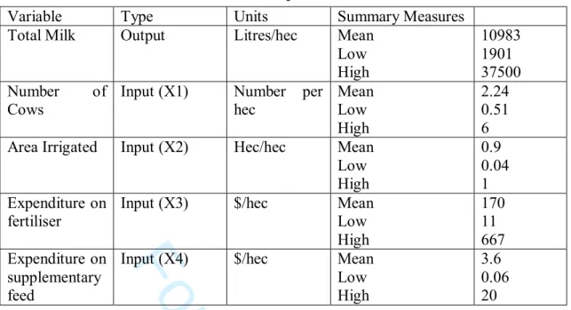
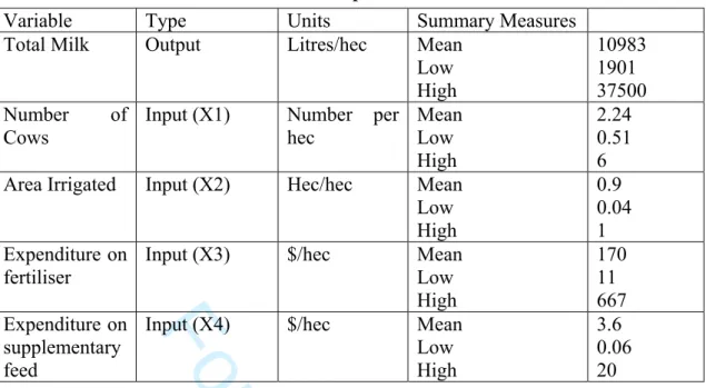
The data used covers the 1999/2000 lactation season. A summary of the data used is presented in Table 1.

{Approximate position of Table 1} 3 4 5 6 7 8 9 10 11 12 13 14 15 16 17 18 19 20 21 22 23 24 25 26 27 28 29 30 31 32 33 34 35 36 37 38 39 40 41 42 43 44 45 46 47 48 49 50 51 52 53 54 55 56 57 58 59 60

For Peer Review

The data set contains one output and four inputs. All data are normalised by farm area so all measures are per hectare. Our output is litres of milk standardised to 4 percent fat. In terms of input use we were able to construct four from the survey. First, we took information on various forms of additional/supplementary feed to construct a dollar measure of purchased feed. Second, the number of cows is a measure of the number of animals in the milking herd. Third, as a measure of irrigation water use, we did not have available the number of megalitres of water applied. Instead we employ area in hectares of the farm irrigated. We would argue that this measure of irrigation water use is a reasonable proxy since all farmers in this region have to pay significant sums of money for water and will equate marginal benefits and costs. There is also a well functioning market in the transfer of water right entitlements between users. Four, we have a composite measure of fertiliser. The fertiliser input is an aggregate measure of various inputs such as Super phosphate, urea and gypsum and is measured as dollars spent per annum.

4.2. Estimation

In terms of the importance of the choice of functional form on estimates of technical efficiency evidence in the literature is mixed. Some authors state that the choice of functional form makes little difference to the estimates of technical efficiency. For example, Ahmad and Bravo-Ureta (1996) found that switching from a Cobb-Douglas functional form to translog yielded almost identical average, minimum and maximum technical efficiency estimates. In terms of statistical properties they rejected the Cobb-Douglas functional form in favour of their simplified translog, but this does not appear to affect efficiency measures derived. Battese and Broca (1997) report similar results. In contrast, Koop et al. (1994) found that the choice of functional did impact on their efficiency estimates when moving from a Cobb-Douglas to an Almost Ideal Model for a cost function. Brümmer (2001) also rejected the use of a Cobb-Douglas compared to a translog production function.

For both CSFA specifications we estimated the generalized likelihood-ratio statistic, which is distributed 2

) (J

χ , to test the null that a Cobb-Douglas frontier was an adequate representation of the data as opposed to a translog (i.e., H0: βij=0). In both cases we were able to reject the null

hypothesis. Given these results a non-constant returns to scale translog frontier production function is estimated. Our production function takes the following form:

3 4 5 6 7 8 9 10 11 12 13 14 15 16 17 18 19 20 21 22 23 24 25 26 27 28 29 30 31 32 33 34 35 36 37 38 39 40 41 42 43 44 45 46 47 48 49 50 51 52 53 54 55 56 57 58 59 60

For Peer Review

∑

∑∑

where βjk = βkj (k≠j) andsubscript i represent the i-th farm and i = 1...241 is the number of farms in the sample. Y represents output of milk per hectare, X1 is the logarithm of the number

of cows per hectare, X2 is the logarithm of the ratio irrigation area to total farm area, X3 is the

logarithm of the cost fertiliser per hectare, and X4 is the logarithm of the cost of

supplementary feed per hectare. 5. Results

Our results are presented in the following order. We begin by examining the production frontier function estimates for the CSFA and BSFA specification. We then examine the point estimates of technical efficiency for all estimation method. Finally, we examine interval estimates of technical efficiency.

5.1. Stochastic Frontier Analysis

We begin by presenting results derived when estimating Equation (12) assuming that ui is a

half-normal (CSFA) and exponential probability distribution (BSFA, CSFA). To simplify the examination of our results, prior to estimation we normalised our sample data by dividing throughout by the sample mean of each variable. Thus, our βi (i=1,2,3,4) estimates are equal to i X Y ∂ ∂ln

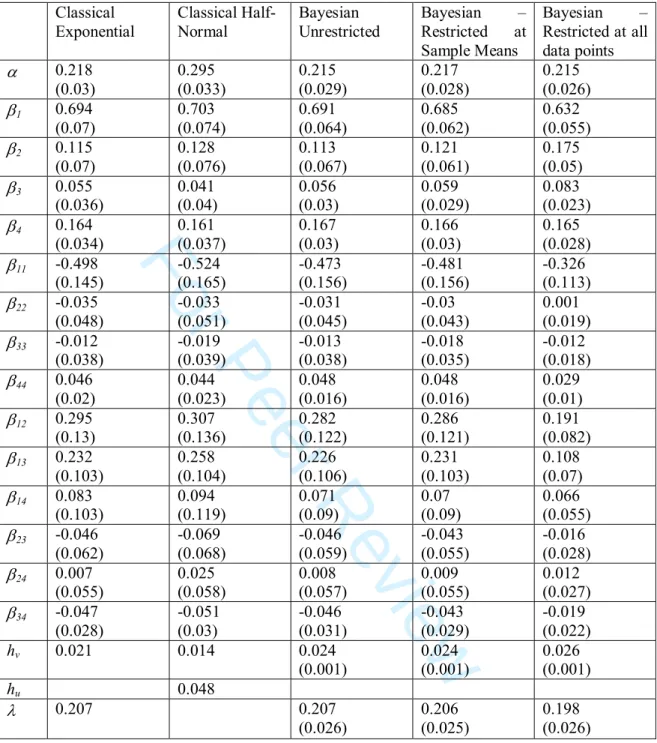
. This also allows us to check if the monotonicity condition is satisfied, by examining the parameter estimates. The production function estimates, Bayesian posterior means and Classical point estimates are reported in Table 2.

{Approximate Position of Table 2}

The results in Table 2 show a great degree of uniformity. The exponential specifications, irrespective if Classical or Bayesian, yielded almost identical results. There are small changes for the Bayesian specification for theory imposed at all data points but these are generally marginal and do not alter the interpretation of the results. For the two Classical specifications there are small differences but these are very minor. The lack of variation in our frontier production function results as we impose theory is not unexpected. We found that the unrestricted data does not conform to monotonicity and/or curvature at for only 19 out 241 data

3 4 5 6 7 8 9 10 11 12 13 14 15 16 17 18 19 20 21 22 23 24 25 26 27 28 29 30 31 32 33 34 35 36 37 38 39 40 41 42 43 44 45 46 47 48 49 50 51 52 53 54 55 56 57 58 59 60

For Peer Review

points. Indeed our frontier parameter estimates suggest that there are many characterisations of the DGP that do equally well. Hence, if interest, is exclusively in the regression parameter estimates, with this data it would really not make much, if any difference, which methodology we employed. Kim and Schmidt (2000) make similar observations regarding all three data sets employed in their analysis.

For the input elasticities for all of the Bayesian specifications reported in Table 2 we find that all of the posterior mass is to the positive side of zero. For the Classical specifications most parameter estimates are statistically different from zero. In all cases, as we would expect for farm level dairy data, the number of cows is the most important contributor to the quantity of milk produced. Both the area irrigated and expenditure on supplementary feed, are statistically significant. The only input in our data that is not significant for most specifications is fertiliser (β3). However, we can see from Table 2 that as we impose the theoretical restrictions every more

tightly the parameter on fertiliser increases. In terms of returns to scale for all specifications the sum of the parameters is very close to one. Indeed, for both CSFA specifications performing a generalized likelihood-ratio statistic, which is distributed 2

) (J

χ , we were unable to reject a null hypothesis of constant returns to scale.

Finally, we can consider the degree of technical inefficiency in our sample. For our Classical models the relative magnitude of variances indicates the existence of technical inefficiency. Similarly, for the Bayesian specifications the estimate of λ is large resulting in the derivation of farm level estimates of technical inefficiency. This statistical significance of this result is provided by the one-sided generalized likelihood-ratio test to test the null hypothesis of no technical inefficiency effects for both CSFA models. In both cases we were able to reject the null hypothesis of no technical inefficiency in our models.

5.2. Comparison of Technical Efficiency Estimates 5.2.1 Mean Estimates

We now examine the farm level technical efficiency estimates (i.e., posterior means for the Bayesian specifications) generated by all the estimation methodologies. As these estimates are frequently the focus of efficiency estimation for policy makers it is important to see if any

3 4 5 6 7 8 9 10 11 12 13 14 15 16 17 18 19 20 21 22 23 24 25 26 27 28 29 30 31 32 33 34 35 36 37 38 39 40 41 42 43 44 45 46 47 48 49 50 51 52 53 54 55 56 57 58 59 60

For Peer Review

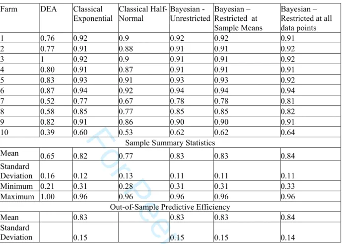
differences between the alternative methodologies can be identified. Technical efficiency estimates for a random sample of ten farms as well as various summary and out-of sample predictive measures are reported in Table 3.

{Approximate Position of Table 3}

In general the results in Table 3 show that the average estimates of technical efficiency for the various methodologies appear to be relatively similar except for DEA that has a lower average. This finding is in keeping with most other comparative studies in the literature. Furthermore, this result is not surprising given the fact that Zhang and Bartels (1998) have shown that for larger samples DEA average estimates of technical efficiency are smaller. Indeed with our data it was found that by randomly reducing sample size that sample average technical efficiency increases. The bottom part of Table 3 reports out-of-sample predictive efficiencies for all exponential specifications. These summary measures are frequently reported in the Bayesian stochastic frontier literature (e.g., van den Broeck et al., 1994, and Koop and Steel, 2001) and are interpreted as measuring the performance of a (maybe hypothetical) firm. Van den Broeck et al. describe this measure as a,” Bayesian counterpart of the classical characteristics of ‘average’ inefficiency.” (p. 279). We have computed these measures following van den Broeck et al. and we find that there is virtually no difference between these measures (Bayesian or Classical) and the summary measures of technical efficiency also reported in Table 3. The equivalence of sample average and out-of-sample estimates is in keeping with the findings of Huang (2004). In summary, even allowing for the lower DEA average all our estimates of technical efficiency are within the range of existing estimates in the literature for dairy farms (Ahmad and Bravo-Ureta, 1996, p. 409). Furthermore, with an average level of technical efficiency from all methodologies of approximately 80 percent, irrespective of estimation methodology, the farms in this sample can be considered very efficient. This result may not be surprising given that dairying in Australia is a mature industry with a well-established extension services distributing information on current best practice on a regular basis. Indeed, it is probably unrealistic to expect higher average estimates of technical efficiency when we allow for exogenous stochastic events that disrupt production such as human error, machinery malfunctions and disease outbreaks.

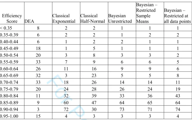
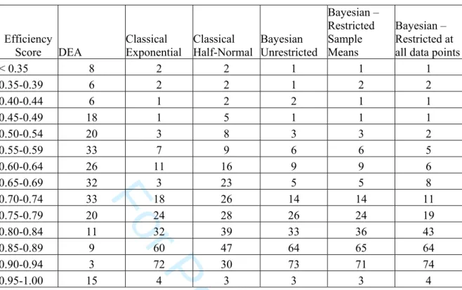
An important aspect of the point estimates of technical efficiency is seen by examining the results in Table 4. 3 4 5 6 7 8 9 10 11 12 13 14 15 16 17 18 19 20 21 22 23 24 25 26 27 28 29 30 31 32 33 34 35 36 37 38 39 40 41 42 43 44 45 46 47 48 49 50 51 52 53 54 55 56 57 58 59 60

For Peer Review

The results in Table 4 show the frequency distribution of technical efficiency for all the methods employed as well as the results for each specific methodology. The most striking feature of the results is that for all frontier methods there is an obvious tail of inefficient farms. This tail is fatter and longer for the DEA results.

From Table 4 we can also identify for CSFA and BSFA the bottom decile of farms. These results, like those of the DEA, indicate that there are a significant number of technically inefficient farms in our sample. But, unlike DEA these farms are part of a much narrower tail and as a result more easily identified. However, the identification of the best performing farms is less clear with CSFA and BSFA, with so many farms yielding technical efficiency estimates clustered around 0.85. As a result we would argue that it is easier to identify those farms that are performing badly compared to farms that are truly best practice. This result is important for applied practitioners of frontier research in that CSFA and BSFA provide a strong characterisation of poorly performing farms. As we noted in the Introduction it is the identification of this very group of farmers that is most important given the recent institutional changes in the Australian dairy industry.

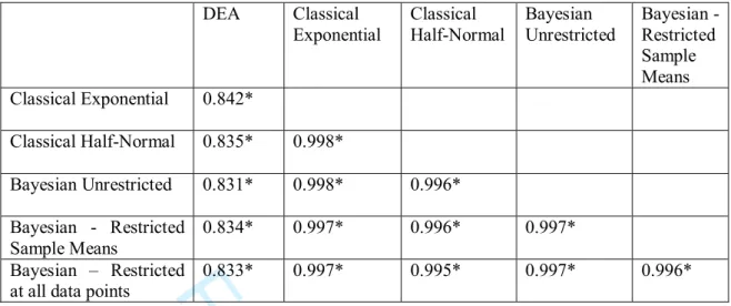
To statistically examine differences between the results generated by the estimation methodologies we use various statistical tests. First, we examine if the sample mean estimates of technical efficiency are statistically different from each other. By performing a simple t-test on the difference between sample means for paired data we find that there are significant differences at the five percent level of significance between DEA and all other methodologies, and between the Classical half-normal specification and all the exponential specifications. However, there are no significant differences between any of the exponential specifications. Second we estimate the Spearman Rank Correlation Coefficient (SRCC) between the technical efficiency estimates to examine if the relative rank of the farms is consistent between the estimation methods, even if the actual estimates differ in terms of magnitude. The null hypothesis tested is that there is no statistical relationship between the two variables. The results for the SRCC are presented in Table 5.

{Approximate Position of Table 5} 3 4 5 6 7 8 9 10 11 12 13 14 15 16 17 18 19 20 21 22 23 24 25 26 27 28 29 30 31 32 33 34 35 36 37 38 39 40 41 42 43 44 45 46 47 48 49 50 51 52 53 54 55 56 57 58 59 60

For Peer Review

In all cases we reject the null hypothesis at the 1% significance level. Hence, the SRCC results indicate that the rank of the farms is statistically invariant to the choice of estimation methodology.

Our findings presented in this section are in keeping the vast majority reported in the literature to date. For example, Kumbhaker and Lovell (2000) note that sample mean efficiencies are sensitive to the distribution assigned to the one-sided error component and there is plenty of evidence to this effect. This finding is mirrored here in terms of the choice of half-normal and exponential distributions. Kumbhaker and Lovell also report that the choice of distribution does not significantly influence the rank of pairs of efficiency estimates. Again our results support Kumbhaker and Lovell. In terms of dairy studies, our results are also in keeping with the literature e.g., Bravo-Ureta and Rieger (1990) and Ahmad and Bravo-Ureta (1996).

5.2.2. Interval Estimates

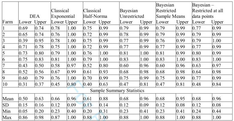
We now extend our comparison of farm level technical efficiency estimates to include interval estimates generated by the alternative frontier estimation methodologies. We estimate 95 percent confidence intervals for the DEA and CSFA specifications and the BSFA credible interval estimates are the 2.5 and 97.5 percentiles of the marginal densities. Our interval estimates presented in Table 6 are for the same ten farms highlighted in Table 3.

{Approximate Position of Table 6}

First consider the DEA confidence interval estimates. The results presented are for ς=0.057. Like Simar and Wilson (1998) we allowed our bootstrap algorithm to search over a large range of values of ς to find the optimal value. There are two features of the confidence interval estimates reported. First, for all farms the resulting confidence interval does not include the point estimate. For example, farm 1 has a point estimate of 0.76 and an upper bound of 0.74. As we previously noted, the DEA program is an upward biased estimator and the confidence interval estimation takes this into account. This finding is entirely consistent with Simar and Wilson (2000). Second, the DEA confidence intervals are in many, but not all, cases significantly narrower than for the other model specifications. This type of result has previously been reported by Brümmer (2001), who attributes it to the alternative modelling philosophies of DEA and stochastic frontiers. DEA is deterministic with data treated as if observed with certainty and random errors in production ignored. Only if the underlying DGP is accurately represented by

3 4 5 6 7 8 9 10 11 12 13 14 15 16 17 18 19 20 21 22 23 24 25 26 27 28 29 30 31 32 33 34 35 36 37 38 39 40 41 42 43 44 45 46 47 48 49 50 51 52 53 54 55 56 57 58 59 60

For Peer Review

our DEA model can we consider these results to be more accurate than those generated by the other methodologies examined.

Turning to the CSFA interval estimates we can see from Table 6 that irrespective of choice of distribution the upper bound is frequently equal or very close to one. This finding is slightly less common for the half-normal specification but with an average estimated upper bound of 0.88 this is still much higher than the DEA results. Again, these results are in keeping with those of Brümmer (2001). When we compare the CSFA exponential with the three BSFA specifications we see that the upper bound estimates are almost identical and the lower bound estimates are only marginally less so.

Finally, a result common to all methods is that the interval estimates for many of the farms in the sample overlap. That is, the intervals for many of the farms include values also included in many of the other farms intervals. This overlapping of the intervals has been identified previously in the literature by Brümmer (2001), and it means that we have to be more conservative about the interpretation we place on our point estimates. This is particularly pronounced for the exponential results that have a large number of farms with an upper bound equal or nearly equal to one.

6. Summary and Conclusions

In this paper we have employed various frontier estimation methodologies to estimate technical efficiency for a sample of irrigated dairy farms. We have examined both point and interval estimates of technical efficiency. For the data examined and the particular methodological specifications employed we find some differences in the results generated by the alternative frontier approaches.

Our point estimate results indicate that there is some evidence of differences between average farm level technical efficiency. We also found that our CSFA and BSFA results provided a sharper distinction of technically inefficient as opposed to technically efficient farms. However, when we examine the relative rank of the farms using the SRCC we find that all methods are statistically significant and close to one, implying that the efficiency rank of farms is consistent across methodologies. Both results are in keeping with previously reported research in much of the literature, which compares frontier estimation methodologies.

3 4 5 6 7 8 9 10 11 12 13 14 15 16 17 18 19 20 21 22 23 24 25 26 27 28 29 30 31 32 33 34 35 36 37 38 39 40 41 42 43 44 45 46 47 48 49 50 51 52 53 54 55 56 57 58 59 60

For Peer Review

From an applied perspective the statistical robustness of the rank of point estimates of technical efficiency is reassuring. It means that analysts will be able to accurately identify those farms operating at lower levels of technical efficiency irrespective of methodology employed. However, when analysts are concerned about the relative level of technical efficiency the statistical differences identified raises serious questions as to the appropriate choice of methodology. But, this finding needs to be qualified when we extend our analysis and also consider interval estimates of technical efficiency. We find that there is significant overlap of intervals for all farms for each methodology employed. The BSFA credible interval estimates are in keeping with CSFA exponential specification. This result parallels closely the findings of Kim and Schmidt (2000). For the DEA confidence intervals, although narrower than the CSFA and BSFA specifications, we would argue is simply a function of the underlying modelling assumptions.

Taken together our interval estimates imply that we can no longer place such a strong interpretation on the point estimates in terms of the actual efficiency score estimate. Instead we have to satisfy ourselves with being able to identify efficient and inefficient groups of farms but for many of the farms we can no longer statistically distinguish their degree of technical efficiency. As previously observed by Brümmer (2001), identification of a group of inefficient farms is easier than identifying efficient farms as so many especially with CSFA and BSFA have upper bound intervals close or equal to one. These results raise questions as to the ability of frontier methods to identify best practice in way frequently demanded by applied researchers and practitioners.

Finally, in the Introduction we addressed the question of the meaning of comparative analysis of different frontier techniques using empirical data. We recognised that identifying the best characterisation of the DGP was a critical step for choosing the correct method, since estimation methods, as employed in this paper, incorporate very different assumptions regarding the DGP. This issue has been examined in the literature before, and continues to be of interest. Gong and Sickles (1992), and more recently, Sickles (2004) have shown using Monte Carlo methods how the preferred choice of method changes depending on the underlying technology (i.e., DGP). Although less than perfect, the sets of criteria proposed by De Borger and Kerstens (1996) and Bauer et al. (1998) also provide some insights into the issue of choice of methodology. We agree with De Borger and Kerstens and Bauer et al. who argue that researchers should attempt to

3 4 5 6 7 8 9 10 11 12 13 14 15 16 17 18 19 20 21 22 23 24 25 26 27 28 29 30 31 32 33 34 35 36 37 38 39 40 41 42 43 44 45 46 47 48 49 50 51 52 53 54 55 56 57 58 59 60

For Peer Review

select reference technologies based on economic arguments. When this is not possible De Borger and Kerstens note that there may well be no solution to identifying the best (most appropriate) reference technology and that we should employ several methods simultaneously and consider a synthesis of the results. Interestingly, this is the approach advocated and being formalised by Sickles. Our findings in this paper add support to this viewpoint. Indeed, we have no a priori reason to assume that one or other frontier method will “better” capture the underlying DGP of our data. The fact that we generate results that provide only minimal evidence regarding any difference between DEA and stochastic frontiers, and that these differences can be explained by the deterministic nature of DEA and its upwardly biased point estimates and narrow interval estimates of technical efficiency, only adds further support to the view that we should consider a synthesis of results.

3 4 5 6 7 8 9 10 11 12 13 14 15 16 17 18 19 20 21 22 23 24 25 26 27 28 29 30 31 32 33 34 35 36 37 38 39 40 41 42 43 44 45 46 47 48 49 50 51 52 53 54 55 56 57 58 59 60

For Peer Review

AATSE (1999). Water and the Australian Economy. A Joint Study Project of the Australian Academy of Technological Science and Engineering and the Institution of Engineers, Australia. AATSE, Melbourne, Victoria.

ACCC (Australian Competition and Consumer Commission) (2001), ‘Impact of Farmgate Deregulation on the Australian Milk Industry’, Monitoring Report, Canberra.

Ahmad, M. and B.E. Bravo-Ureta (1996). Technical Efficiency Measures for Dairy Farms Using Panel Data: A Comparison of Alternative Model Specifications, Journal of Productivity Analysis, 7, 399-415.

Aigner, D.J., C.A.K. Lovell, and P. Schmidt. (1977). Formulation and Estimation of Stochastic Frontier Production Function Models, Journal of Econometrics, 6, 21-37.

Battese, G.E. and S.S. Broca (1997). Functional Forms of Stochastic Frontier Production Functions and Models for Technical Inefficiency Effects: A Comparative Study for Wheat Farmers in Pakistan, Journal of Productivity Analysis, 8, 395-414.

Battese, G.E. and T.J. Coelli (1988). Prediction of Firm-Level Technical Efficiencies With a Generalised Frontier Production Function and Panel Data, Journal of Econometrics, 38, 387-399.

Battese, G.E., A. Heshmati and L. Hjalmaarsson (2000). Efficiency of Labour Use in the Swedish Banking Industry: A Stochastic Frontier Approach, Empirical Economics, 25, 623-640. Bauer, P.W., A.N. Berger, G.D. Ferrier and D.B. Humphrey (1998). Consistency Conditions for Regulatory Analysis of Financial Institutions: A Comparison of Frontier Efficiency Methods, Journal of Economics and Business, 50: 85-114.

Bravo-Ureta, B.E. and L. Rieger (1990). Alternative Production Frontier Methodologies and Dairy Farm Efficiency, Journal of Agricultural Economics, 41, 215-226.

Brümmer, B. (2001). Estimating Confidence Intervals for Technical Efficiency: The Case of Private Farms in Slovenia, European Review of Agricultural Economics, 28, 285-306.

Casella, G. and E. George (1992). Explaining the Gibbs Sampler, The American Statistician, 46, 167-174.

Chib C. and E. Greenberg, (1995). Understanding the Metropolis-Hastings Algorithm. The American Statistician, November, 49, 4:327-335

Cloutier, L.M. and R. Rowley. (1993). Relative Technical Efficiency: Data Envelopment Analysis and Quebec’s Dairy Farms, Canadian Journal of Agricultural Economics, 41, 169-176.

3 4 5 6 7 8 9 10 11 12 13 14 15 16 17 18 19 20 21 22 23 24 25 26 27 28 29 30 31 32 33 34 35 36 37 38 39 40 41 42 43 44 45 46 47 48 49 50 51 52 53 54 55 56 57 58 59 60

For Peer Review

Coelli, T.J., D.S. Prasada Rao and G.E. Battese. (1998). An Introduction to Efficiency and Productivity Analysis. Kluwer Academic Publishers, London.

Cuesta, R.A. (2000). A Production Model with Firm-Specific Temporal Variation in Technical Inefficiency: With Application to Spanish Dairy Farms, Journal of Productivity Analysis, 13, 139-158.

Cummins, J.D. and H. Zi (1998). Comparison of Frontier Efficiency Methods: An Application to the US Life Insurance Industry, Journal of Productivity Analysis, 10, 131-152.

De Borger, B. and K. Kerstens (1996). Cost Efficiency of Belgian Local Governments: A Comparative Analysis of FDH, DEA and Econometric Approaches, Regional Science and Urban Economics, 26, 145-170.

DRDC (1999). Improving Efficiency of Water Use. Research Note 69, Dairy Research and Development Council, http://www.drdc.com.au.

DRDC (2000). Natural Resource Management on Australian Dairy Farms: A Survey of Australian Dairy Farmers, Dairy Research and Development Council, http://www.drdc.com.au. Edwards, G. (2003), The Story of Deregulation in the Dairy Industry, Australian Journal of Agricultural and Resource Economics, 47, 1-24.

Farrell, M.J. (1957). The Measurement of Productive Efficiency, Journal of the Royal Statistical Society, Series A, 120, 253-281.

Fernández, C., J. Osiewalski and M.F.J. Steel (1997). On the Use of Panel Data in Stochastic Frontier Models with Improper Priors, Journal of Econometrics, 79, 169-193.

Fernández, C., G. Koop and M.F.J. Steel. (2000). A Bayesian Analysis of Multiple-Output Production Frontiers, Journal of Econometrics, 98, 47-79.

Fernández, C., G. Koop and M.F.J. Steel (2002). Multiple-Output Production with Undesirable Outputs: An Application to Nitrogen Surplus in Agriculture, Journal of the American Statistical Association, 97, 432-442.

Fraser, I.M. and D. Cordina (1999). An Application of Data Envelopment Analysis to Irrigated Dairy Farms in Northern Victoria, Australia, Agricultural Systems, 59, 267-282.

Gong, B.H. and R.C. Sickles (1992). Finite Sample Evidence on the Performance of Stochastic Frontiers and Data Envelopment Analysis Using Panel Data, Journal of Econometrics, 51, 259-284.

Hjalmarsson, L.J, S.C. Kumbhakar and A. Heshmati (1996). DEA, DFA and SFA: A Comparison, Journal of Productivity Analysis, 7, 303-327.

3 4 5 6 7 8 9 10 11 12 13 14 15 16 17 18 19 20 21 22 23 24 25 26 27 28 29 30 31 32 33 34 35 36 37 38 39 40 41 42 43 44 45 46 47 48 49 50 51 52 53 54 55 56 57 58 59 60

For Peer Review

Horrace, W.C. and P. Schmidt (1996). Confidence Statements for Efficiency Estimates from Stochastic Frontier Models, Journal of Productivity Analysis, 7, 257-282.

Huang, H.C (2004). Estimation of Technical Inefficiencies with Heterogeneous Technologies, Journal of Productivity Analysis, 21: 277-296.

Jaforullah, M., and J. Whiteman. (1999). Scale Efficiency in the New Zealand Dairy Industry: A Non-Parametric Approach, Australian Journal of Agricultural and Resources Economics, 43, 523-542.

Jondrow, J., C.A.Knox Lovell, I.S. Materov and P. Schmidt (1982). On the estimation of Technical Inefficiency in the Stochastic Frontier Production Function Model, Journal of Econometrics, 19, 233-238.

Karagiannis, G., P. Midmore and V. Tzouvelekas (2002). Separating Technical Change from Time-Varying Technical Inefficiency in the Absence of Distributional Assumptions, Journal of Productivity Analysis, 18, 23-38.

Kim, Y. and P. Schmidt (2000). A Review and Empirical Comparison of Bayesian and Classical Approaches to Inference on Efficiency Levels in Stochastic Frontier Models with Panel Data. Journal of Productivity Analysis, 14, 91-118.

Kleit, A.N. and D. Terrell (2001). Measuring Potential Efficiency Gains fro Deregulation of Electricity Generation: A Bayesian Approach, Review of Economics and Statistics, 83, 523-530. Koop, G, J. Osiewalski and M.F.J. Steel (1994). Bayesian Efficiency Analysis with a Flexible Form: The AIM Cost Function, Journal of Business and Economic Statistics, 12, 339-346.

Koop, G, J. Osiewalski and M.F.J. Steel (1997). Bayesian Efficiency Analysis Through Individual Effects: Hospital Cost Frontiers, Journal of Econometrics, 76, 77-105.

Koop, G.J., M.F.J. Steel and J. Osiewalski (1995). Posterior Analysis of Stochastic Frontier Models Using Gibbs Sampling, Computational Statistics, 10, 353-373.

Koop, G.J. and M.J.F. Steel (2001). Bayesian Analysis of Stochastic Frontier, in Baltagi, B. (ed.) A Companion to Theoretical Econometrics, Blackwells, Mass.

Kurkalova, L.A. and A. Carriquiry (2003). Input- and Output-Orientated Technical Efficiency of Ukrainian Collective Farms, 1989-1992: Bayesian Analysis of a Stochastic Frontier Model, Journal of Productivity Analysis, 20, 191-211.

Kumbhakar, S.C. and C.A.K. Lovell (2000). Stochastic Frontier Analysis. Cambridge University Press, Cambridge, UK.

Meeusen, W. and J. van den Broeck (1977). Efficiency Estimation from Cobb-Douglas Production Functions with Composed Error, International Economic Review, 18, 435-444.

3 4 5 6 7 8 9 10 11 12 13 14 15 16 17 18 19 20 21 22 23 24 25 26 27 28 29 30 31 32 33 34 35 36 37 38 39 40 41 42 43 44 45 46 47 48 49 50 51 52 53 54 55 56 57 58 59 60