Few-shot Classifier GAN

Few-shot Classifier GAN

Adamu Ali-Gombe1 Eyad Elyan1 Yann Savoye1 Chrisina Jayne2

1_{Robert Gordon University} 2_{Oxford Brookes University}

Abstract— Fine-grained image classification with a few-shot classifier is a highly challenging open problem at the core of a numerous data labeling applications. In this paper, we present Few-shot Classifier Generative Adversarial Network as an approach for few-shot classification. We address the problem of few-shot classification by designing a GAN in which the discriminator and the generator compete to output labeled data in any case. In contrast to previous methods, our techniques generate then classify images into multiple fake or real classes. A key innovation of our adversarial approach is to allow fine-grained classification using multiple fake classes with semi-supervised deep learning. A major strength of our techniques lies in its label-agnostic characteristic, in the sense that the system handles both labeled and unlabeled data during training. We validate quantitatively our few-shot classifier on the MNIST and SVHN datasets by varying the ratio of labeled data over unlabeled data in the training set. Our quantitative analysis demonstrates that our techniques produce better classification performance when using multiple fake classes and larger amount of unlabelled data.

1. Introduction

Image classification [35] is a challenging task requiring a large amount of labeled dataset to train accurate models at optimal performance. With the advent of Deep Learning technologies, there is a huge demand in obtaining massive labeled dataset [21], [17]. One major limitation is that massively annotating labels is a labor-intensive task [4]. Data augmentation is an alternative strategy to bypass the unavailability of labeled training data. Unfortunately, such models trained only on synthesized data largely under-perform.

In this paper, we are interested in performing few-shot classification [3] because when only a few labeled samples can be acquired, unlabeled data could also be considered. Also, we are motivated to achieve generation and co-classification, in the sense that the generation will improve the classification and the classification will improve the generation cooperatively.

Our work falls into the general problem domain of data labeling [29]. In particular, fine-grained classification [16] is an important problem with practical applications. Despite much recent progress, it remains a challenge to generalize classification and generation with lack of labeled data. Our key observation is that incorporating more fake classes plays an important role in training the GAN models at a

finer-grained level, which may improve the overall performance. In this paper, we present a step towards fine-grained few-shot classification with the Generative Adversarial Net-works. In contrast to the state of the art, our GAN is more versatile and less restrictive in term of input and output.

The core idea is to carefully fuse supervised and un-supervised learning via switchers within the connections of the GAN. Therefore, the GAN can be fed with labeled or unlabelled input data. Our proposed method classifies real samples into real classes and then isolate fake samples into their respective unknown fake classes. We solve this problem by leveraging fine-grained classification thanks to two mech-anisms: fake class embedding and multiple fake classes. Drawing inspiration from AC-GAN [27] and SGAN [26], our key idea is to associate classes with new samples by conditioning generation on class embedding. In contrast to previous work, our method seeks to classify real samples into predefined classes and further isolate fake samples into their respective fake classes, taking benefit of semi-supervised learning to improve the classifier accuracy.

In this paper, the technical contribution is a novel GAN architecture taking as input labeled and labeled training data and performing fine-grained classification thanks to a multi-ple fake classes strategy. Our method is designed to handle image generation losses and unconditional generation when unlabeled data are used during training. To the best of our knowledge, our model is the only one able to achieve fine-grained classification along image generation comparing to other GANs in the zoo. We demonstrate the effectiveness of our system by evaluating our solution on publicly available datasets. Our results suggest that incorporating multiple fake classes in the GAN models improve the overall performance, especially in presence of few labeled data.

2. Related Works

Data labeling can be done automatically [2], [6]. The construction of fully labeled dataset is supported by learning methods such as semi-supervised [20], one-shot [34] and active learning [7]. In particular, semi-supervised learning combines labeled with unlabelled data. Also, data augmen-tation [13] is an alternative strategy to bypass the absence of labeled training data by transforming original samples. Finally, data synthesis generates artificial data by training models exclusively on synthesized data [5], [31]. Naturally, the intuitive zero-sum game principle of generative adver-sarial networks (GANs) is an appealing strategy for data labeling.

(a) GAN [15] (b) CGAN [23] (c) SGAN [26] (d) ACGAN [27] (e) Our FSCGAN Figure 1: The GAN zoo. We compare the architecture of Vanilla GAN [15], CGAN [23] SGAN [26], ACGAN [27] with our Few-Shot Classifier GAN (FSCGAN). In our design,C∗

is the set of all classes, andX∗

is the set of all samples (fake and real). In our GAN, we add network switchers (depicted as⊗) forcing the network to switch to the suitable learning mode (supervised or unsupervised) for each mini-batch training. We highlight in cyan color the differences between all GANs with the firstly introduced Vanilla GAN.

The GAN [15] is defined as a generative adversarial model that can be trained [14]. The discriminator tries to estimate losses from predictions and ground truth, whereas the generator estimates log likelihood of the distributions over data. Table 1 outlines the properties of various GANs related to our work. The first Vanilla GAN [15] introduces the Kullback-Leibler divergence as a distance-based distri-bution similarity to produce highly-detailed images. TABLE 1: Comparison of properties of our GAN against state-of-the-art GANs.

Model Supervised Unsupervised Few labels Multi fake classes

Vanilla GAN[15] 7 X 7 7 S-GAN[26] X X 7 7 AC-GAN[27] X X 7 7 C-GAN[23] X 7 7 7 CatGAN[32] X X X 7 CC-GAN[10] X X X 7 SS-GAN[33] X X X 7 TAC-GAN[9] X X 7 7

Few-shot C-GAN(Our) X X X X

GAN has a lot of applications targeted for images processing, such as image data augmentation [25], high-resolution image generation [18] image reconstruction [30], text-2-image generation [28], natural image generation [11]. However, variants of GANs have been also proposed for classification [20], categories classification [27], semi su-pervised labeling [26] and other domains [12], [11].

Nevertheless, tailoring GANs for classification is a te-dious task [8]. Vanilla GAN [15] is an unsupervised ad-versarial model that allows only to output if a sample is real/fake. Therefore, no classification can be performed by the discriminator of Vanilla GAN since this model only accepts unlabeled data as input. Our method differs by performing generation in conjunction with classification. However, Conditional GAN [23] generates data conditioned on class labels via label embeddings in both discriminator

and generator. Similar to Categorical GAN [32] (CatGAN), our method integrate a classification loss function to learn a classifier from unlabeled or partially labeled data.

Conditioning on labels brings to light the possibility of semi-supervised classification using GANs by forcing the discriminator network to output class labels. In semi-supervised GANs [26] (SGAN), the training is realized by combining a single fake class with known classes. This additional fake class is required to categorize samples from the generator. In our approach, we combine conditioning and embedding to cope with the well-known limitation of semi-supervised GANs, namely being unable to handle unlabelled data. Auxiliary Classifier GAN (AC-GAN) [27] is also conditioned on the class labels to generate visually plausible images. Our work is close to the AC-GAN in the sense that we exploit label conditioning. However, our classifier GAN is not restricted to outputting a single class label for every sample.

Contrary to AC-GAN and CGAN that only rely on full labeled datasets, our model can perform label conditioning for unlabeled data and output sub-class labels even for fake images. Our model is also auxiliary because we output a numeric value deciding if the image is real or fake, and multiple fake classes. Comparing to all GANs in Table 1, our model is the only model ables to perform fine-grained classification along image generation so far, even if the expected class is not provided for training. We leverage this fine-grained property by injecting multiple fake classes with embedding. Moreover, the key difference of our approach against AC-GAN and SGAN is that our classification is not limited to real classes. Our approach combines supervised and unsupervised learning to handle both unlabeled and labeled data.

3. Methods

3.1. Fake Class Encoding

”Real” refers to label or images provided as part of the training set, while ”fake” refers to generated label or images. The set of real labels C={0,· · ·, N−1} for the N classes are extracted from the training data (indexed from 0 to 9 for digits). For each class c in the training data, a corresponding fake class label c+ is added automatically as described in the following procedure. The index of each digit is converted into a one-hot encoding vector. Then, we generate a set of fake class labels C+ _{by accommodating}

a longer vector representation. The one-hot encoding of the real classes is padded with |C| zeros shifted to the right. From this one-hot representation, the corresponding fake class is generated by padding zeros at the left of the real label. For example, if the real label0 is encoded over |C| bits as 1000000000, we now represent this class by

10000000000000000000. Then, the corresponding fake label is 00000000001000000000. The resulting set of all labels is denotedC∗_{=C ∪ C}+_.

3.2. Few-shot Classifier GAN

Our Few-shot Classifier GAN consists of two Convo-lutional Neural Networks competing against each other: a generator model G and a discriminator model D, where the discriminator tries to classify real objects and objects synthesized by the generator, and the generator attempts to confuse the discriminator. This model is designed to classify real and fake samples. This optimization problem requires a min-max solution obtained by solving the overall functional:

min

D maxG Vf shot(D, G) (1)

where D and G mimic a two-players minmax game with value function Vf shot(D, G). Then, the optimal solution is

reached when both models can not make a significant gain over its opponent.

Similar to classical AC-GAN, the generator G takes as input a random noise vector z ∈ Rd where d is the vector size and c is a label when the corresponding class is available. In the absence of class labels in the training set, G takes onlyz as input. G is trained to be an image producer aiming to generate sampled images expected to lie within the distribution of the training data. The classifier is incorporated within the discriminator model D to produce better samples. Then,D is trained to discriminate between image generated by Gagainst real training images.

The value functionVf shot(D, G)is defined as a

piece-wise function acting as a network switcher, as follows: Vf shot(D, G) = ( ˜ C∗_{={∅} : V} gan(D, G) ˜ C∗_{6={∅} : V} acgan(D, G) (2)

whereC˜∗_{is the class labels set involved in the current batch}

andVgan(D, G)is the expected value of the unconditioned

probabilities overD andG. Alternatively,Vacgan(D, G)is

the expected value of the conditioned probabilities over D and G depending on labels for classification. The network switcherVf shotenforces the GAN model to perform

uncon-ditional discrimination (Vgan) in the absence of labels and

to perform conditional discrimination (Vacgan).

Vgan(D, G) =Ex∼pdata(x)[logD(x)]

+Ez∼pz(z)[log (1−D(G(z)))]

(3) where the prior distribution is denoted by pz and z is the

set of prior noise drawn from a uniform distribution. The generator samples the latent representation variable zonly to generate images. Subsequently, Vacgan is activated when

GandDare conditioned with the class labels setC∗_during

training.

Vacgan(D, G) =Ls+Lc (4)

where Ls and Lc respectively denotes the log-likelihood

of the expected sampling and classification. Formally, the sampling lossLsand the classification loss Lc write as:

Ls=E[logP(S=real|Xreal)]

+E[logP(S =f ake|Xf ake)]

(5)

Lc =E[logP(C=c|Xreal)]

+E[logP(C=c|Xf ake)]

(6) The discriminator D(X) = (P(S|X), P(C|X)) iso-lates fake versus real samples and then performs the clas-sification of all samples whether real or fake. P(S|X) is a probability distribution over samples and P(C|X) is probability distribution over labels. Xf ake = G(c, z) is a

batch of generated images and Xreal is a batch of real

images used to train the discriminator D. In the presence of labels, the conditioning C is based on the class labels for the sampling and uses both labeled and unlabeled data. Our GAN has two set of outputs: a scalar determining if the image is real or fake and a set of discrete values representing the labels corresponding to real or fake samples.

3.3. Network Switcher

We inject the network switcher inside our deep neu-ral architecture to manage multiple learning strategies by forcing the learning to switch to the desired mode for the training. This solution is better than trivially switching between two different models (namely, AC-GAN and GAN) by avoiding duplication of generators and discriminators. In particular, this binary switcher create an algorithm branch within the computational graph to switch to a supervised or unsupervised training. This network switcher is expressed as an exclusive OR operator (XOR) ensuring that the learning strategy fits the nature of the given batch. As shown in the Figure 1, the switcher is depicted using the⊗operator.

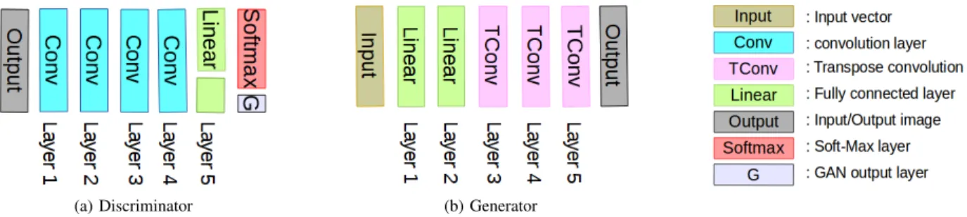
(a) Discriminator (b) Generator

Figure 2:The Few-shot Classifier GAN generated images by transpose convolution to avoid up-sample resizing. Both diagrams show the arrangement of layers for the architecture of the Discriminator and the Generator. The discriminator produces two outputs: a classifier output determining the class, and an output determining the type of image (real or fake).

3.4. G and D Black Boxes

Our few-shot classifier is a Deep Convolutional GANs to produce better visual quality samples. The Generator and Discriminator are both expressed as deep convolutional neural networks with a fixed number of layers, leaky Relu activation functions and hyper-parameters. We tune the hyper-parameters and the number of layers to fit the desired image resolution. Figure 2 depicts the inner architecture of the Generator and the Discriminator.

In the generator G, we use a series of transpose con-volutions with varying strides to upsample images at the desired resolution. The first two layers of the generator are fully connected with no in-between batch normalization. The outputs of the second layer are reshaped into an7×7 image with 128 channels. The third layer is a transpose convolution using a single stride and outputs a7×7 image with 256 channels. The forth layer is a transpose convolution with a stride of 2 outputting an 14×14 image with 128 channels. Finally, the final layer uses a transpose convolution outputting an28×28image with a single channel.

The discriminator D is a conventional CNN down-sampling image batches into a feature vector representation suitable for classification. The discriminator is composed of four convolution layers with strides of 2 in each layer. We use batch normalization between layers to accelerate the convergence, excepting in the final layer. The subsequent layers are two parallel linear layers: a classification output and a GAN output. The classification layer returns logits while the GAN layer returns the sigmoid activated output (fake or real).

3.5. Dual Training

The training procedure is summarized in the provided pseudo-code (Algorithm 1). The procedure described in the Algorithm 1 takes as input data and label batches. Each batch is tailored with given ratio of labeled to unlabeled data. The training process is performed by alternating between supervised and unsupervised training since the amount of labeled samples may differ in each epoch.

In Algorithm 1, the number of epochs is e = 500. The inner loops among labeled and unlabeled samples are

balanced to guarantee the stability of the loss function. The first loop (k steps) iterates over labeled data only by per-forming stochastic gradient descent over the Discriminator and Generator via the discriminator. This loop evaluates the sampling and classification losses functions (line 6). The overall loss is updated at the end of each iteration within the inner loop. Similarly, the second loop (jsteps) iterates over unlabeled data, but only sampling loss is evaluated before updating the overall loss. The number of iteration k andj depends proportionally on the ratio of labeled and unlabeled data to produce an important-based sampling. However, if the training dataset is balanced then k=j.

Algorithm 1Training Algorithm

1: procedure TRAIN(data batches, label batches) 2: foreepochs do

3: for k stepsdo

4: Fetch next labeled mini batches

5: Perform Stochastic Gradient Descent onD 6: Perform Stochastic Gradient Descent onG

7: Evaluate(Ls,Lc)

8: UpdateD andGlosses

9: end for

10: forj steps do

11: Fetch next unlabeled data mini batches 12: Perform Stochastic Gradient Descent onD

13: Perform Stochastic Gradient Descent onG

14: Evaluate(Vs)

15: Update D andGlosses

16: end for

17: end for

18: end procedure

The discriminator D is trained to maximize Ls+Lc

while the generator G is trained to minimize the entropy between Ls and Lc. Our discriminator D is trained with

image batches from G and real images taken from the training data. We update the discriminatorD by minimizing the overall loss function. We update the generator G by minimizing the overall loss function.

4. Experimental Results and Evaluation

An extensive experimental analysis is conducted to eval-uate the accuracy of the proposed model with multiple fake classes. The proposed GAN architecture is used to perform all experiments in which the ratio of unlabeled samples and labeled samples is varied during the training process. Experiments were ran in aNVIDIA DGX-1supercomputer with multiple GPUs using the TensorFlow framework. Finally, performances of the proposed model are reported in term of accuracy for a variety of training configurations. 4.1. Datasets Tuning

We run our experiments over two state-of-the art datasets of 32×32 images, namely the MNIST dataset [22] and the SVHN dataset [24]. We have selected these real-world datasets because they are well-suited database for training and testing at minimal efforts on pre-processing and for-matting. Unlabeled data are derived from the datasets by neglecting provided labels.

The MNIST dataset is large database composed of a train set (60000 images) and a test set (10000 images) with size-normalized, centered, fixed-size and single-channel im-ages representing handwritten digits. Each digit has it cor-responding label. In our experiments, the train and the validation sets are fused to create a new training set to evaluated our GAN. Using this dataset, our experiments based on varying the number of unlabeled samples start by considering all labels from the training set. Then, the number of labeled samples is decreased by 10k at each run until the lower bound of 50k unlabeled and 10k labeled samples is reached.

The Street View House Numbers SVHN dataset is sig-nificantly harder and more challenging. TheSVHNis a real-world dataset (73k train set and a 26k test set) composed of three-channels noisy images of house numbers obtained from Google Street. The class distribution in the training set varies between 5k to 13k instance per class. Using this dataset, our experiments start with 73k full-labeled samples and the testing is performed only on 10k randomly-selected samples from the test set. The unlabeled set is enriched with 10k samples selected from the train set at each pass until the lower bound of 60k unlabeled samples is reached. 4.2. Setup and Parameters

We have implemented our approach using

TensorFlow [1]. We use 10 million trainable (labeled) parameters and 30 million trainable (unlabeled) parameters. We bypass the unbalanced data problem by collecting an equal number of unlabeled samples from each class when designing our training dataset for our labeled-to-unlabeled experiments. Even if the size of labeled samples set decreases, it is worth noting that the size of the training set remains unmodified along the experiments. However, the training set is extended with fake classes for multiple fake class experiments. During the testing phase, the learned

classifier is evaluated over 10k samples from hold out real test samples.

A batch size of 32 is used for all datasets and all experiments. We normalize all input before the training. We use the classical Adam optimizer [19] with a learning rate of 10-3 _{for the gradient descent optimization of the} generator and the discriminator. Also, we consider a prior vector of 100 dimensions from the uniform distribution. Since grid search is computationally expensive with these hyper-parameters, we use random search.

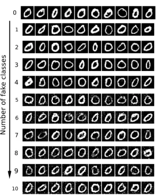
Figure 3: For the digit 0, we display the output of our proposed GAN without fake classes (first row). The second row represents the output obtained while considering a single fake. Then, we increase the number of fake classes for all other following rows (top to bottom). Visual results show that the pixel corruptions grow proportionally when multiple fake classes are considered during the training.

4.3. Performance Evaluation

We evaluated the accuracy of the output obtained by our learned classifier with multiple fake classes in comparison with the output produced by our learned classifier with only a single fake. The evaluation metric we employ to measure the accuracy of the trained classifier is defined as the total number of correctly classified test samples divided by the overall number of test samples.

We reported the quantitative results for this accuracy in Table 2 and 3 for experiments conducted over 10k test samples by varying number of class labels during the training. Sample images are collected at the end of the overall training. We depict generated images from training on MNIST and SVHN with 50k and 60k unlabeled data

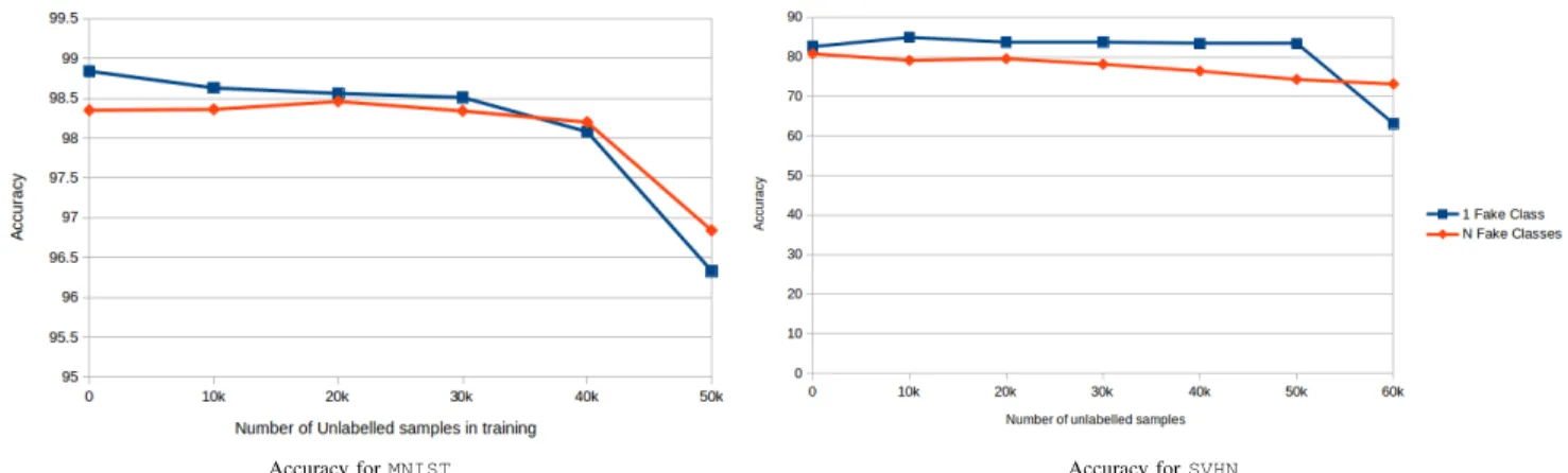
Accuracy forMNIST Accuracy forSVHN

Figure 4: We plot the accuracy of our Few-shot Classifier GAN in function of the number of unlabeled samples. For this test, we trained our GAN with semi-supervised learning over theMNISTandSVHNdatasets. The multiple fake classes mode outperforms the single fake class mode in presence of 70% of the data are unlabeled.

respectively in Figure 5. The performance of our Few-shot CGAN is summarized in Figure 4.

We conducted further examination of numerical results by carrying out a pair t-test analysis on the reported accu-racies. As assumption, we take the null hypothesis that the two modes (single fake class and multiple fake classes) are indistinguishable. The mean of two outputs is similar with a confidence is 5%. A p-value of 0.5841 for the MNIST

dataset and a p-value of 0.2097 for theSVHN. Since these p-values are greater than 0.05, we do not reject the null hypothesis.

TABLE 2:We report the precision accuracy of semi-supervised learning applied on theMNIST dataset with different configura-tions of fake classes on 10k hold out samples.

Unlabelled Samples Single Fake Class Multiple Fake classes

0 98.84 98.35 10k 98.63 98.36 20k 98.56 98.46 30k 98.51 98.34 40k 98.08 98.20 50k 96.33 96.84

Further experiments are conducted by varying the num-ber of fake classes from 0 to N (where N is the total number of real classes) to examine how fake classes affect the generation of images. For this experiment, the GAN is re-trained from scratch using bias sampling. Figure 3 shows the effect on the quality of image generation when the number of fake classes increases. Samples are collected when the training is completed.

5. Discussion

We observe that the accuracy drops when the number of labeled samples decrease in training. For both publicly available SVHN and MNIST datasets. A wider margin is observed during experiments with theSVHNdataset because

of the challenging characteristics of this specific dataset. For both datasets, ourFew-shot GANoutperforms the classifica-tion process inmultiple fake classesmode with the presence of fully labeled data. Also, our Few-shot GAN performs better inmultiple fake classesmode than insingle fake class mode, in the presence of 70 % of the data are unlabeled. Our techniques perform significantly better with a factor 10 when 60k unlabeled samples are fed to our GAN.

TABLE 3: We report the precision accuracy of semi-supervised learning applied on theSVHNdataset with different configurations of fake classes on 10k hold out samples.

Unlabelled Samples Single Fake Class Multiple Fake classes

0 82.55 80.76 10k 84.90 79.07 20k 83.67 79.49 30k 83.68 78.11 40k 83.34 76.38 50K 83.30 74.25 60k 63.11 73.10

Unfortunately, generated samples exhibit visual artifacts when our GAN is used in the multiple fake class mode when tested on theSVHNdataset. Visual qualitative results show that the quantity of visual artifacts grows proportionally when multiple fake classes are considered during the train-ing. Moreover, we notice the apparition of artifacts when unlabeled samples become dominant over labeled samples and when the GAN relies less on the classification loss. Better performances are also observed when the generator is trained on not too good and not too poor samples. Finally, we observe that bias sampling does not significantly improves the quality of generated samples. We suggest to devise a deeper architecture or training on more epochs to solve this problem.

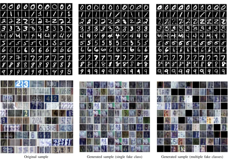
Original sample Generated sample (single fake class) Generated sample (multiple fake classes)

Figure 5: The first row contains MNISTsamples and the second row containsSVHN samples. On the left-hand side, we display real image samples from the training data, samples from training with a single fake class are displayed in the middle. Finally, we display generated sample images when trained with multiple fake classes on the right-hand side. Generated samples are obtained from 50k and 60k unlabeled training data onMNISTandSVHNrespectively.

6. Conclusions

Fine-tuning labeling is currently done manually. In the few-shot context where we lack labeled training data, clas-sifying images and labeling data is still a tough problem. In this work, we focused on the design of a novel adversarial architecture incorporating latent label embedding, network switchers and multiple fake classes to solve the problem of zero-shot classification. One of the greatest appeals of our approach is its label-agnostic property. Also, our GAN supports a wide range of strategies from fully supervised, semi-supervised to weakly supervised learning that was not possible with any alternative GAN previously.

In contrast to other fine-grained classification techniques, our method takes advantage of the generator to trick the discriminator into classifying generated data along with their labels whatever the input is. We leverage this property by exploiting the continuum of the known labeling space. One of the central differences is that we do not learn how to represent real labeled data but how to learn powerful representations from unlabeled data. The most important

aspect of our few-shot classifier GAN is its capability to output unknown sub-categories (namely the fake classes) for which we have no training examples.

As a result, our proposed GAN is a useful tool to learn a stable classification in the presence of few labeled examples mixed with a significant amount of unlabeled examples. An important advantage of our method can switch between full supervised learning and semi-supervised learning thanks to the network switchers. Although our evaluation confirms that discriminated samples improve the overall accuracy when the dataset lacks labeled samples. In most cases, our work suggests that the proposed approach performs similarly to traditional GAN in the presence of a sufficient amount labels and provides better results in the absence of labeled samples during the training phase. The main limitation of our technique is that the generated sample quality could be damaged when multiple fake classes are used.

In conclusion, we believe that this work demonstrates the feasibility of training data generation in GAN with less label training data required to achieve desired performance. We are confident that our method provides valuable insights

into the fine-grained classification problem, and open a new horizon to perform deep learning with less amount of data. Finally, a more sophisticated design of loss functions are needed to support the generation of images at higher visual plausibility. An important advance toward this direction would be a new family of fake loss functions optimized for the human visual perception.

References

[1] Mart´ın Abadi, Ashish Agarwal, Paul Barham, Eugene Brevdo, Zhifeng Chen, Craig Citro, Greg S. Corrado, Andy Davis, Jeffrey Dean, Matthieu Devin, Sanjay Ghemawat, Ian Goodfellow, Andrew Harp, Geoffrey Irving, Michael Isard, Yangqing Jia, Rafal Jozefowicz, Lukasz Kaiser, Manjunath Kudlur, Josh Levenberg, Dan Man´e, Rajat Monga, Sherry Moore, Derek Murray, Chris Olah, Mike Schuster, Jonathon Shlens, Benoit Steiner, Ilya Sutskever, Kunal Talwar, Paul Tucker, Vincent Vanhoucke, Vijay Vasudevan, Fernanda Vi´egas, Oriol Vinyals, Pete Warden, Martin Wattenberg, Martin Wicke, Yuan Yu, and Xiaoqiang Zheng. Tensorflow: Large-scale machine learning on heterogeneous systems. 2015.

[2] Yalong Bai, Kuiyuan Yang, Wei Yu, Chang Xu, Wei-Ying Ma, and Tiejun Zhao. Automatic image dataset construction from click-through logs using deep neural network. InInternational Conference on Multimedia, 2015.

[3] Rinu Boney and Alexander Ilin. Semi-supervised few-shot learning with prototypical networks. CoRR, 2017.

[4] Bastiaan J Boom, Phoenix X Huang, Jiyin He, and Robert B Fisher. Supporting ground-truth annotation of image datasets using cluster-ing. InInternational Conference on Pattern Recognition, 2012. [5] Konstantinos Bousmalis, Nathan Silberman, David Dohan, Dumitru

Erhan, and Dilip Krishnan. Unsupervised pixel-level domain adapta-tion with generative adversarial networks. arXiv, 2016.

[6] Liang-Chieh Chen, Sanja Fidler, Alan L Yuille, and Raquel Urtasun. Beat the mturkers: Automatic image labeling from weak 3d super-vision. InConference on Computer Vision and Pattern Recognition, 2014.

[7] Brendan Collins, Jia Deng, Kai Li, and Li Fei-Fei. Towards scalable dataset construction: An active learning approach. ECCV, 2008. [8] Zihang Dai, Zhilin Yang, Fan Yang, William W Cohen, and Ruslan

Salakhutdinov. Good semi-supervised learning that requires a bad gan. arXiv, 2017.

[9] Ayushman Dash, John Cristian Borges Gamboa, Sheraz Ahmed, Muhammad Zeshan Afzal, and Marcus Liwicki. Tac-gan-text con-ditioned auxiliary classifier generative adversarial network. arXiv, 2017.

[10] Emily Denton, Sam Gross, and Rob Fergus. Semi-supervised learn-ing with context-conditional generative adversarial networks. arXiv, 2016.

[11] Emily L Denton, Soumith Chintala, Rob Fergus, et al. Deep genera-tive image models using a laplacian pyramid of adversarial networks. InAdvances in Neural Information Processing Systems, 2015. [12] Jeff Donahue, Philipp Kr¨ahenb¨uhl, and Trevor Darrell. Adversarial

feature learning. arXiv, 2016.

[13] Alexey Dosovitskiy, Jost Tobias Springenberg, Martin Riedmiller, and Thomas Brox. Discriminative unsupervised feature learning with convolutional neural networks. InAdvances in Neural Information Processing Systems, 2014.

[14] Vincent Dumoulin, Ishmael Belghazi, Ben Poole, Alex Lamb, Martin Arjovsky, Olivier Mastropietro, and Aaron Courville. Adversarially learned inference. arXiv, 2016.

[15] Ian Goodfellow, Jean Pouget-Abadie, Mehdi Mirza, Bing Xu, David Warde-Farley, Sherjil Ozair, Aaron Courville, and Yoshua Bengio. Generative adversarial nets. In Advances in Neural Information Processing Systems, 2014.

[16] Xiangteng He and Yuxin Peng. Weakly supervised learning of part selection model with spatial constraints for fine-grained image classification. InAAAI, 2017.

[17] Geoffrey E Hinton, Simon Osindero, and Yee-Whye Teh. A fast learning algorithm for deep belief nets. Neural Computation, 2006. [18] Tero Karras, Timo Aila, Samuli Laine, and Jaakko Lehtinen.

Progres-sive growing of gans for improved quality, stability, and variation.

arXiv, 2017.

[19] Diederik Kingma and Jimmy Ba. Adam: A method for stochastic optimization.arXiv, 2014.

[20] Diederik P Kingma, Shakir Mohamed, Danilo Jimenez Rezende, and Max Welling. Semi-supervised learning with deep generative models. InAdvances in Neural Information Processing Systems, 2014. [21] Alex Krizhevsky, Ilya Sutskever, and Geoffrey E. Hinton. Imagenet

classification with deep convolutional neural networks. InAdvances in Neural Information Processing Systems. 2012.

[22] Yann LeCun, Corinna Cortes, and Christopher JC Burges. Mnist handwritten digit database. AT&T Labs, 2010.

[23] Mehdi Mirza and Simon Osindero. Conditional generative adversarial nets. arXiv, 2014.

[24] Yuval Netzer, Tao Wang, Adam Coates, Alessandro Bissacco, Bo Wu, and Andrew Y Ng. Reading digits in natural images with unsu-pervised feature learning. InNIPS workshop on deep learning and unsupervised feature learning, 2011.

[25] Dong Nie, Roger Trullo, Jun Lian, Caroline Petitjean, Su Ruan, Qian Wang, and Dinggang Shen. Medical image synthesis with context-aware generative adversarial networks. InInternational Conference on Medical Image Computing and Computer-Assisted Intervention, 2017.

[26] Augustus Odena. Semi-supervised learning with generative adversar-ial networks. arXiv, 2016.

[27] Augustus Odena, Christopher Olah, and Jonathon Shlens. Condi-tional image synthesis with auxiliary classifier gans. International Conference on Machine Learning, 2017.

[28] Scott Reed, Zeynep Akata, Xinchen Yan, Lajanugen Logeswaran, Bernt Schiele, and Honglak Lee. Generative adversarial text to image synthesis. InInternational Conference on Machine Learning, 2016. [29] Bryan C Russell, Antonio Torralba, Kevin P Murphy, and William T

Freeman. Labelme: a database and web-based tool for image anno-tation. International Journal of Computer Vision, 2008.

[30] Kevin Schawinski, Ce Zhang, Hantian Zhang, Lucas Fowler, and Gokula Krishnan Santhanam. Generative adversarial networks recover features in astrophysical images of galaxies beyond the deconvolution limit. Monthly Notices of the Royal Astronomical Society: Letters, 2017.

[31] Ashish Shrivastava, Tomas Pfister, Oncel Tuzel, Josh Susskind, Wenda Wang, and Russ Webb. Learning from simulated and un-supervised images through adversarial training. arXiv, 2016. [32] Jost Tobias Springenberg. Unsupervised and semi-supervised learning

with categorical generative adversarial networks. arXiv, 2015. [33] Kumar Sricharan, Raja Bala, Matthew Shreve, Hui Ding, Kumar

Saketh, and Jin Sun. Semi-supervised conditional gans.arXiv, 2017. [34] Oriol Vinyals, Charles Blundell, Tim Lillicrap, Daan Wierstra, et al. Matching networks for one shot learning. InAdvances in Neural Information Processing Systems, 2016.

[35] Shengke Xue and Xinyu Jin. Robust classwise and projective low-rank representation for image classification.Signal, Image and Video Processing, 2018.