Semi-Supervised Online Multi-Kernel Similarity
Learning for Image Retrieval
Jianqing Liang, Qinghua Hu, Senior Member, IEEE, Wenwu Wang, and Yahong Han
Abstract—Metric learning plays a fundamental role in the
fields of multimedia retrieval and pattern recognition. Recently, an online multi-kernel similarity (OMKS) learning method has been presented for content-based image retrieval (CBIR), which was shown to be promising for capturing the intrinsic non-linear relations within multimodal features from large-scale data. However, the similarity function in this method is learned only from labeled images. In this paper, we present a new framework to exploit unlabeled images and develop a semi-supervised OMKS algorithm. The proposed method is a multi-stage algorithm consisting of feature selection, selective ensemble learning, active sample selection and triplet generation. The novel aspects of our work are the introduction of classification confidence to evaluate the labeling process and select the reliably labeled images to train the metric function, and a method for reliable triplet generation, where a new criterion for sample selection is used to improve the accuracy of label prediction for unlabelled images. Our proposed method offers advantages in challenging scenarios, in particular, for a small set of labeled images with high-dimensional features. Experimental results demonstrate the effectiveness of the proposed method as compared with several baseline methods.
Index Terms—Image retrieval, metric learning, similarity
learning, multi-kernel learning, semi-supervised, OMKS, S-SOMKS.
I. INTRODUCTION
W
ITH the rapid growth of multimedia data such as images and videos, measuring the similarity between visual objects becomes an increasingly important task in a variety of applications including classification, clustering and retrieval [1–3]. Conventionally, this can be achieved by using pre-defined functions, such as the Euclidean distance and co-sine similarity. With these functions, however, the underlying distribution of the data is often implicitly assumed. As a result, the complex intrinsic structures within the data may not be well captured by these functions.To address this problem, an increasing amount of effort has been made to learn an appropriate metric directly from the data, for applications such as content-based image retrieval (CBIR), which is our focus here. In the pioneering work by Xing et al [4], metric learning is formulated as a convex
J. Liang, Q. Hu and Y. Han are with the School of Computer Science and Technology, Tianjin University, Tianjin 300072, China (e-mail: [email protected]; [email protected]; [email protected].)
W. Wang is with Center for Vision Speech and Signal Processing, and De-partment of Electronic Engineering, Faculty of Engineering and Physical Sci-ences, University of Surrey, United Kingdom (e-mail: [email protected].) This work is partly supported by National Program on Key Basic Research Project under Grant 2013CB329304, National Natural Science Foundation of China under Grants 61222210 and 61432011, and Q. Hu is supported by New Century Excellent Talents in University under Grant NCET-12-0399.
optimization problem with a set of similarity and dissimilarity constraints, where a global Mahalanobis distance is learned by keeping similar pairs of objects close to each other while dissimilar pairs apart from each other [5]. This earlier work has inspired the development of a number of methods for learning global linear metrics, such as the information-theoretic method [6, 7], nearest neighbor classification method [8], Laplace regularized metric learning (LRML) [9], and more recently, the geometric mean metric learning (GMML) method [10].
These global metric learning techniques, however, are often limited for large-scale problems due to their high computa-tional complexity. They may also suffer from the issue of the so-called curse of dimensionality [11]. To overcome these limitations, a number of algorithms have been presented for learning local metrics [12–16], which are deemed to be more flexible for capturing the variations across multiple feature spaces, and offering better performance, as compared with global metrics. However, the local metrics tend to be prone to the problem of overfitting [5].
The aforementioned algorithms aim to learn linear metrics which may have limitations in characterising the relations between the different modalities in multi-modal data, since they often have non-linear relations, and are in different spaces and dimensions. To address these issues, multiple kernel tech-niques have been introduced [17–20], by mapping the images to a high-dimensional feature space with a nonlinear kernel matrix. In [17], an optimal ensemble of kernel transformations is learned for integrating features of multiple modalities into a unified space. However, it is computationally expensive, and consequently not applicable to high-dimensional and large-scale datasets. In [18], a multi-modal distance metric learning framework is proposed by projecting data from different modalities into a latent feature space based on the multi-wing harmonium model. In [19], a weighted kernel embedding technique is presented for metric learning, which is shown to be flexible in combining multiple features. Using multiple kernel techniques, the complementary nature of different fea-tures extracted from an image can be better exploited. For this reason, multi-kernel learning techniques are also considered in our work.
In applications with large-scale data, however, the algo-rithms discussed above are often limited in their scalability. The computational complexity and memory requirement of these algorithms may increase significantly when dealing with large-scale data [5]. To address this challenge, online techniques have been proposed in e.g. [21–23]. In [23], an online multiple kernel similarity learning (OMKS) algorithm is presented, where a flexible nonlinear proximity function
with multiple kernels is learned in a supervised manner and applied to visual search. In [21], an online multimodal deep similarity learning (OMDSL) framework is proposed to improve multimedia similarity search by integrating multi-ple deep networks with a scalable online scheme. In [22], an online multi-modal distance metric learning (OMDML) scheme is proposed, where the optimal metrics are learned in individual modality space and the weights for combining different modalities are obtained with a joint formulation. These algorithms rely overwhelmingly on the availability of labeled data in their training. In practice, however, labelling data by human is time consuming and costly. In addition, the labels provided by different labellers are not always consistent and could be noisy. Therefore, it is highly desirable if the large-scale unlabelled data could be directly used in metric learning.
The use of unlabelled data in metric learning has been considered in previous work e.g. [9, 24, 25]. However, these methods were proposed for learning global Mahalanobis met-rics, but not for local metrics. In this paper, inspired by the OMKS algorithm in [23], we propose a novel multi-stage semi-supervised online multi-kernel similarity (SSOMK-S) learning framework for using the unlabelled data in metric learning. More specifically, we present a new method for triplet generation to allow the incorporation of the unlabelled data in the OMKS algorithm. An important challenge in the use of unlabelled data comes from the risk associated with the unreliability and noise in the training samples. To counter this problem, a new active sample selection method based on the concept of margin is proposed for measuring the classification confidence. This leads to a new method for reliable triplet generation where the labeling process is evaluated in order to select the reliably labeled images for learning the metric function. To our knowledge, such an idea has not yet been exploited in metric learning.
The remainder of this paper is organized as follows. Section II briefly summarises the baseline OMKS algorithm in [23]. In Section III, we introduce our proposed SSOMKS learning framework which is a multi-stage method including feature selection, selective ensemble learning, active sample selection, and triplet generation. Section IV presents experimental results on both qualitative and quantitative analysis, including the evaluation of each stage of the proposed method and its comparison with several baseline methods. We conclude the paper with an outlook for future work in Section V.
II. THEOMKS LEARNINGMETHOD
In this section, we give a brief introduction to the OMKS algorithm presented in [23].
Suppose there is a kernel κ(·,·) and the corresponding Hilbert space H, and consider a linear operatorL: H 7→ H
that maps a functionf ∈ Hto another oneL[f]∈ H. Assume there is a collection ofmkernel functionsK={κi:χ×χ→
R, i = 1, . . . , m}. A similarity function for visual search is defined as f(q, p) = m P i=1 θiSi(q, p) = m P i=1
θihκi(q,·), Li[κi(p,·)]iHκi (1)
where q ∈ χ is a query image, and p ∈ χ is an
image in the pooling set to be retrieved. Si(q, p) = hκi(q,·), Li[κi(p,·)]iHκi is the similarity function based on the linear operatorLi. The goal is to learn the weights{θi}m
i=1 and the linear operators{Li}m
i=1 simultaneously. Given a set ofT triplets{(pt, p+t, p
−
t)}Tt=1whereptshould be more similar top+t than top
−
t, the objective function that
needs to be optimised is given as follows
min θ∈△{Lmini}mi=1 1 2 m P i=1 θikLik2 HS+C T P t=1 ℓ(f(pt, p+t)−f(pt, p − t)) (2) where k · kHS is the Hilbert Schmidt norm of the linear
operator, C ≥0 is the loss parameter,ℓ(z) is the hinge loss and△is defined as
△={θ∈Rm+|θTem= 1} (3)
To solve the problem (2), online learning techniques are introduced. In particular, for kernel κi, the corresponding weightθi and linear operatorLi are updated in T iterations. That is, when the tth triplet (pt, p+t, p
−
t) arrives, the weight θi(t−1) and linear operatorLt−1,i in kernelκi are updated
to obtainθi(t)andLt,i, respectively.
Starting withL0,i=I,Lt,i for thetth triplet is updated as Lt,i=Lt−1,i+τt,iZt (4)
whereh∈ H, Zt[h](·) =κ(pt,·)(h(p+t)−h(p−t))∈ L(L=
{L:H 7→ H, L is a linear operator} is the space including linear operators inH) andτt,i is computed as
τt,i= min{C,max{0,1−SLt−1,i(pt,p
+ t)+SLt−1,i(pt,p − t)} κ(pt,pt)(κ(p+t,p + t)−2κ(p + t,p−t)+κ(p−t,p−t)) } (5)
Then, the weight of kernelκi is updated as
θi(t) =θi(t−1)βzi(t) (6)
where β ∈ (0,1) is a discounting parameter which is used to penalize the kernel that makes incorrect predictions in each iteration, andzi(t) equals to 1 when SLt−1,i(pt, p
+
t)− SLt−1,i(pt, p
−
t)≤0, and 0 otherwise.
The OMKS algorithm is a supervised algorithm trained with labelled data. The triplet generation does not consider the use of unlabeled data. To address this issue, we propose a new semi-supervised multi-stage learning framework, by extending the OMKS algorithm to the scenario where only a small amount of training data is labelled while the majority of the data are unlabeled, as discussed next.
III. PROPOSEDSEMI-SUPERVISEDOMKS LEARNING
METHOD
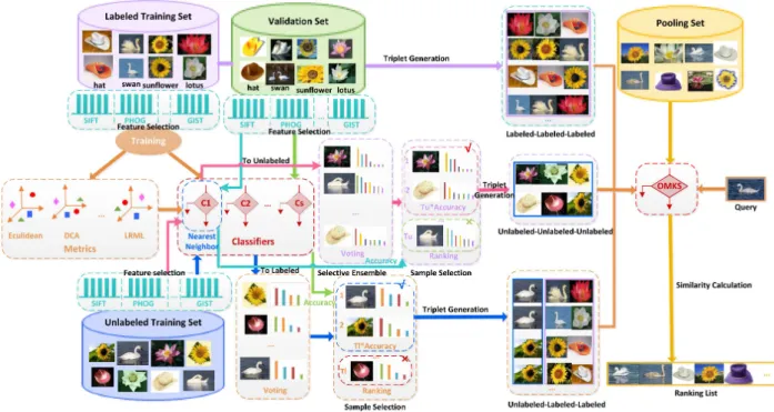
Our new framework of SSOMKS is a multi-stage method consisting of feature selection, selective ensemble learning, active sample selection, and triplet generation. The key con-tribution in this framework is a new method for generating the triplets, as well as a new approach for controlling the potential risk in using unlabelled data with active sample selection based on the concept of margin.
The diagram of the proposed method is shown in Fig. 1. First, feature selection is performed to obtain discriminative
Fig. 1. Flow chart of the semi-supervised online multiple kernel similarity framework for image retrieval. For each image in the dataset, we extract 9 types of features (e.g., SIFT, PHOG, etc.) and then select several dimensions in each modality. Then, we learn metrics (e.g., DCA, LRML, etc.) as well as classifiers (e.g., random forest, subspace, etc.) for each modality with labeled training set. Specifically, we apply the learned metrics for constructing the nearest neighbor classifier. To select appropriate classifiers, selective ensemble learning is performed on validation set. Unlabeled training set is viewed as test data. By searching the nearest and farthest class of these images with the selected classifiers, we obtain unlabeled-labeled-labeled triplets. Unlabeled-unlabeled-unlabeled triplets can be generated by finding the nearest and farthest samples, while labeled-labeled-labeled triplets are produced by supervision information of labeled training set. For the first two types of triplets, we also make the first attempt to perform active sample selection with margin. Please refer to Section IV for details.
feature space. Then, ensemble learning is introduced to train the classifiers for each type of features, and the classifiers that offer better classification performance are selected. Third, an active sample selection method is proposed to ensure that the samples with correctly predicted labels are used. Finally, the triplets with these selected samples are generated to perform metric learning for visual search. The details of each stage are discussed below.
A. Feature Selection
High-dimensional multiple features extracted from images may contain redundant information. Feature selection is help-ful for choosing the discriminative dimensions in the feature space. Here, we apply the Multi-Cluster Feature Selection (MCFS) [26] method, as it is computationally efficient and also independent of the choice of classifiers.
Given an image training set X ={x1,x2, . . . ,xN},xi ∈
RD ofN images withD dimensions in K clusters. Suppose
we want to select d dimensions and the number of nearest neighbors is set as p. For each image xi, we construct a p
nearest neighbor graph by finding its pnearest neighbors and form an edge between xi and its neighbors. We define the
weight matrixW on the graph and a diagonal matrixDbased on W,Dii =PjWij. The graph LapalcianL=D−W.
Solve the generalized eigen-problem [27]
Ly=λDy (7)
LetY = [y1, . . . ,yK]be the topK eigenvectors
correspond-ing to the smallest eigenvalues λ = [λ1, . . . , λK]. For each
cluster, we solve the equivalent formulation of LASSO using Least Angle Regression (LARs) algorithm [28] by specifying the cardinality asd min ak k yk−XTakk2 s.t. kakk1=d (8) Then we getKsparse coefficient vectors{ak}Kk=1∈RD. The MCFS score for each featurej is computed as
M CF S(j) = max
k |ak,j| (9)
We obtain the topdfeatures according to the ranking.
B. Selective Ensemble Learning
Following feature selection, classification is performed to predict the labels of unlabelled samples. Here, ensemble learn-ing is employed due to its advantage over a slearn-ingle classifier in its generalization ability to unseen data [29]. The performance of ensemble learning algorithms may vary. It was shown that ensembling many of the available learners can be better than ensembling all of them [30]. Therefore, selective ensemble learning is introduced to remove the under-performed learners. Here, we adopt the Margin based Pruning (MP) [31] algorithm to select proper classifiers. An advantage with the MP algo-rithm is that the distribution of the sample intervals can be further optimised during the process of ensemble selection. The MP procedure is discussed as follows.
SupposeX ={x1,x2, . . . ,xN}is the training image set, h1, . . . , hL are the base classifiers,yi is the true class label of
xi, and yijˆ (j = 1,2, . . . , L)is the classification decision of
xi estimated by the classifierhj. The margin ofxiis defined
as m(xi) = L P j=1 wjΛij (10)
wherewj is the weight of hj,Λij =
1,if yi = ˆyij
−1,if yi6= ˆyij
Forxi∈X, its classification loss is defined as
l(xi) = [1−m(xi)]2 (11)
The loss of classification is computed as
l(X) = N P i=1 l(xi) =ku−Dwk22 (12) where u = [1,· · ·,1]T N×1,w = [w1,· · · , wL]TL×1,D = {Λij}N×L.
The L2-norm regularization is added to the loss function [32]
Fw=ku−Dwk2
2+λkwk2 (13)
The weightswj (j= 1,2, . . . , L)can be obtained by minimiz-ingFw using open software packages such as [33]. Then, the classifiershsj(sj= 1,2, . . . , L)are ranked in terms of the de-scending order of the weightswj (j= 1,2, . . . , L). After this, we compute the average precisionψjwith{hs1, hs2, . . . , hsj}. Finally, {hs1, hs2, . . . , hsB} are the selected classifiers with
B = max
j∈{1,...,L}ψj.
C. Sample Selection with Classification Confidence
For unlabelled data, the labels predicted by voting in the above section may not be reliable. As a result, the triplet could be wrongly generated, which can have negative impact on both the computational efficiency and learning performance of metric learning. To address this problem, we propose a new technique to select samples, based on the concept of margin, which has been previously used to measure the confidence of classification. If a trained model gives a large margin, it will have a higher degree of confidence and reliability. Inspired by the work in [34–37], we introduce the concept of classification confidence to sample selection. Our method is based on three hypotheses. First, each selected classifier has considerable classification ability, which means it is better than random guess. Second, the accuracy is positively related to the votes of the largest class. Third, the accuracy is positively related to the margin between the first and the second largest class.
Assume theLclassifiers are independent, whereL= 2k+1
is odd. LetXibe a variable indicating whether the classifica-tion by theith classifier is correct or not. If the prediction accu-racy of each classifier is p, then we haveXi∼Bernouli(p), and the number of correct classifications with the ensemble majority voting method is Y =
L
P
i=1
Xi∼binomial(L, p)[38].
The majority vote accuracy is
Pmajority(L)= L P i=k+1 L i pi(1−p)L−i (14)
It has been shown that the sequence {Pmajority(2k+1)} strictly increase when p > 0.5 [39]. In addition,
limk→∞Pmajority(2k+1) = 1, and the prediction accuracy of the ensemble voting method converges to 1 when p > 0.5. As the probability for the largest number of votes may be smaller than half, Equation (14) is the lower bound of the actual probability.
Suppose there are N u unlabeled training images, B clas-sifiers andK classes. We introduce a parameterc to balance between the maximum and the margin, and define the criterion for selection ascmax+ (1−c)margin. We denote the voting accuracy of validation images with these B classifiers as
Accv. After ranking theN uimages in a descending order of
cmax+(1−c)margin, we select the topN u∗Accvunlabeled images to generate triplets.
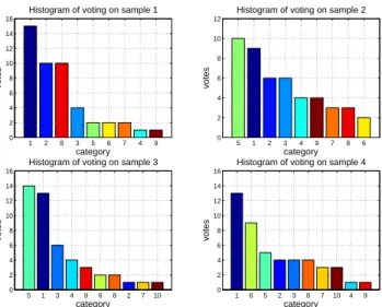
1 2 8 3 5 6 7 4 9 0 2 4 6 8 10 12 14 16 category votes
Histogram of voting on sample 1
5 1 2 3 4 9 7 8 6 0 2 4 6 8 10 12 category votes
Histogram of voting on sample 2
5 1 3 4 9 6 8 2 7 10 0 2 4 6 8 10 12 14 16 category votes
Histogram of voting on sample 3
1 6 5 2 3 8 7 10 4 9 0 2 4 6 8 10 12 14 16 category votes
Histogram of voting on sample 4
Fig. 2. Voting results of samples in Class 1. Each classifier outputs a label for each sample. The final predicted class is the one which gets the most votes. Sample 1 and 4 fall into Class 1, while sample 2 and 3 fall into Class 5.
Fig. 2 gives an example of the voting results for four unlabeled samples from Class 1. We observe that only sample 1 and 4 are correctly classified. Two incorrectly labeled samples will be introduced with all classifiers. The accuracy on validation set is 37.5%. Thus we may select 2 out of 4 samples with relevant strategies. If we adopt the max criterion, then sample 1 and 3 are chosen, introducing one mistake. If we use the margin ormax+margin criterion, then sample 1 and 4 are selected without a mistake. This illustrates that our sample selection strategy can improve classification accuracy.
D. Triplet Generation
To exploit a certain unlabeled imagexifor metric learning,
it is necessary to find its nearest neighbor xj and farthest
imagexk to generate the triplet(xi,xj,xk).
Given an unlabeled sample xi, the triplets can be divided
into two types, i.e., labeled-labeled and unlabeled-unlabeled-unlabeled ones according to whether xj and xk
are labeled or not. For the former, we first label xi with
the selected base classifiers. The farthest class is the one to which the farthest sample found with learned metrics belongs. Then,xjs can be the labeled training samples that belong to
the same class with xi, whereasxks are the labeled training
are required to find the nearest and farthest samples to xi
in unlabeled training set. Without supervision information, we consider exploiting the learned metrics. Therefore,xjs are the
nearest unlabeled samples whilexks are the farthest unlabeled
ones obtained by the metrics.
E. Summary of the Proposed SSOMKS Learning Framework
The implementation steps of the proposed SSOMKS method are summarised in Algorithm 1. It can be seen that the proposed SSOMKS differs from the OMKS algorithm in the process on how the triplet is generated. In the proposed method both the labeled and unlabeled images are used to learn a metric, while in the baseline OMKS method, only the labeled images are considered.
Algorithm 1 The SSOMKS algorithm Input:
Labeled training set with M modalitiesDl={Dl j}Mj=1; Unlabeled training setDu={Du
j}Mj=1; Validation setDv={Dv j}Mj=1; Trade-off parameterc; Output: f(q, p); 1: forj= 1toM do
2: Feature selection from the jth modality Dl
j (Section III-A), then we get the labeled, unlabeled training set
and validation setDsl
j ,Djsu,Dsvj ;
3: Learn metrics and train classifiers with Dsl j ; 4: end for
5: Select classifiers withDsv (Section III-B);
6: Vote forDsu, computemaxandmarginfor each sample;
7: RankDsuin a descending order ofcmax+(1−c)margin, then perform sample selection (Section III-C);
8: Exploit the selected samples to generate triplets (Section
III-D);
9: Input these triplets to the OMKS framework;
10: Outputf(q, p).
In constrast to [23], where a theoretical analysis is presented for the OMKS method, we do not yet have a theoretical proof for the convergence property of the proposed SSOMKS method. However, a simulation study is provided in Section IV-A for the analysis of its convergence.
IV. EXPERIMENTS
In this section, we evaluate the performance of SSOMKS and compare it with several baseline methods. We first intro-duce the experimental setting and then show the results as well as the analysis to these results.
A. Experimental Setting
1) Datasets and Experiment: We conduct the experiments
on image datasets including Corel [40], ImageCLEF1, Indoor2,
1http://imageclef.org/.
2http://web.mit.edu/torralba/www/indoor.html.
Caltech2563, Flickr4 and Oxford Buildings5. We pick 10,
20 and 50 classes in Caltech256 to form three subsets, i.e. Caltech10, Caltech20 and Caltech50, respectively. In other datasets, we pick 10 classes. For each dataset, the number of images for each class equals the number of images of the class that has the minimum size in its sample set. We select half of the images for training, 10% for validation, 10% for query, and the remaining 30% for retrieval evaluation. The experiment is performed on a machine with 3.40 GHz Intel processor, 8 GB memory, and the Matlab software.
2) Descriptors and Kernels: Both global and local feature
descriptors are extracted to represent images. The global fea-tures we tested include: (1) color histogram (256 dimensions for gray images and 768 dimensions for color images); (2) GLCM coefficients (16 dimensions); (3) Local Binary Pattern (59 dimensions); and (4) GIST features (512 dimensions). The local features we used include: (1) SIFT; (2) dense-SIFT; (3) SURF; (4) Geometric Blur; and (5) PHOG (680 dimensions). We set the vocabulary size as 200 to represent Bag-of-Words (BOW) features except for the PHOG descriptor. Since CNN is effective for image content representation and is trained with color images, we extract DCNN feature (4096 dimensions) using CaffeNet, except for the dataset ImageCLEF. Then we apply PCA to each type of features and retain the first 50 principle components. The full dimension of the original features is retained if it is smaller than 50.
Based on these features, we construct 4 kernels [23]: RBF kernel: κ(x, x′) = exp(−kx−x′k2
rσ2 ), where the pa-rameter r is the mean of the pairwise distance and σ ∈ {10−2,2∗10−2,4∗10−2} is the scale parameter.
Cosine similarity: κ(x, x′) = hx,x′i
kxk2kx′k2. To ensure the similarity value in the range of [0, 1], we adopt κ(x, x′) =
0.5kxhkx,x′i
2kx′k2 + 0.5.
3) Base Classifiers: We perform the feature selection
al-gorithm MCFS on each feature and select 50 dimensions. All dimensions are kept if the original feature is less than 50. To make predictions for unlabeled training images, we construct a series of base classifiers for each kind of feature, i.e. Adaboost M1 [41] + CART [42], discriminative analysis [43], random forest [44], subspace as well as nearest neighbor with Euclidean distance, RCA [6], DCA [40], LRML [9] and SERAPH [15] metrics.
TABLE I
PARAMETERSETTING OFSSOMKS
Parameter d k num λ C β
Value 50 20 50 10000 [0,1] (0,1)
4) Evaluation Criteria: For each query image, we can rank
all of the test images according to their similarities. Here we use the mean Average Precision (mAP) to evaluate the performance of retrieval. Given a query and its R retrieved images, the Average Precision is defined as
AP =L1 R P r=1 prec(r)δ(r) (15) 3http://www.vision.caltech.edu/Image DataSets/Caltech256/. 4http://press.liacs.nl/mirflickr/mirdownload.html. 5http://www.robots.ox.ac.uk/vgg/data/oxbuildings/index.html.
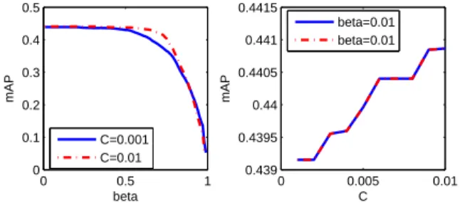
0 0.5 1 0 0.1 0.2 0.3 0.4 0.5 beta mAP C=0.001 C=0.01 0 0.005 0.01 0.439 0.4395 0.44 0.4405 0.441 0.4415 C mAP beta=0.01 beta=0.01
Fig. 3. Retrieval performance vs. parameterCandβfor the Indoor dataset. The solid lines represent the first round of parameter tuning and dashed lines represent the second round. In each round, first we fix parameter C
while tuningβ, and then we fix parameterβwhile tuning parameterC. The algorithm converges after two rounds. Noticing that the curves in the right column are not smooth, and this seems to suggest that the algorithm converges to a local optimum.
whereLis the size of the relevant images in the retrieved set,
prec(r)is the precision at therth position, andδ(r)represents whether the rth retrieved image is relevant to the query or
not. δ(r) = 1 when they are relevant; δ(r) = 0, otherwise.
The mAP is defined based on the average AP values of all the queries. R is set as the number of images for each class in the pooling set.
5) Compared Methods and Parameter Setting: We compare
SSOMKS with the following state-of-the-art metric learning algorithms. For each metric, we concatenate all types of features, and then report the retrieval result.
• DCA: An efficient supervised metric learning scheme which can exploit both positive and negative constraints [40].
• LRML: A semi-supervised distance metric learning tech-nique that integrates both labeled and unlabelled samples into an effective graph regularization framework [9].
• OASIS: A supervised online dual approach that learns a
bilinear similarity measure over sparse representations [45].
•EMR: A scalable graph-based manifold ranking algorithm for image retrieval [46].
•ITML: An information-theoretic method which minimizes the differential relative entropy between two multivariate Gaussians with constraints [7].
•DML-eig: An efficient eigenvalue optimization framework for metric learning [16].
• OMKS: An efficient online metric learning algorithm which learns a flexible nonlinear proximity function with multiple kernels for improving visual search [23].
• SERAPH: An information-theoretic metric learning ap-proach that does not rely on the manifold assumption [15].
•HDS: A deep learning framework to learn hash codes and image representations in a point-wise manner [47].
Table I shows the parameter setting of SSOMKS. It was ob-served that MCFS performs well when the number of selected features is smaller than 50 [26]. Therefore, we setdas 50. The parameterkof kNN in LRML controls the number of nearest neighbors linked in a KNN graph. Commonly, it is tuned in 5-20. As the number of labeled images per class is greater than 20, we setk as 20. For ensemble learning methods including Adaboost, random forest and subspace, we set num as 50. The trade-off parameterλin MP is used to avoid overfitting. By tuning it in{10−4,10−3,10−2,10−1,1,10,102,103,104} on the validation set, we set it as 10000. The choices of C
andβ follow from OMKS.
Fig. 3 gives an example of parameter tuning. We only tune several key parameters and set all the remaining to default values. In particular, we set the regularization parametersγs,
γd as 1 due to the lack of prior information and vary the parameterkof kNN in LRML in the range of 5-20. We set the number of the landmarks pickedpin EMR as 50 after tuning
TABLE II
THE CLASSIFICATION ACCURACY(%)ONCOREL, IMAGECLEFANDINDOOR DATASETS WHEN THE TRAINING RATIO IS20%.
Datasets Triplets MP MP+margin MP+max MP+max+margin Corel unlabeled-labeled-labeled 54.67 71.01 76.81 75.36 unlabeled-unlabeled-unlabeled 54.67 60.71 69.05 69.05 ImageCLEF unlabeled-labeled-labeled 85.00 94.06 93.07 94.06 unlabeled-unlabeled-unlabeled 82.50 81.13 81.13 81.13 Indoor unlabeled-labeled-labeled 50.00 60.00 60.00 57.78 unlabeled-unlabeled-unlabeled 58.89 62.22 64.44 62.22 0 50 100 150 200 12 14 16 18 20 22 24 26 28 # of features NMI (%) All Features MCFS PCA LS CSE+GS DLSR−FS
(a) SIFT (Corel)
0 50 100 150 200 20 22 24 26 28 30 32 34 36 # of features
NMI (%) All Features
MCFS PCA LS CSE+GS DLSR−FS
(b) Gray histogram (ImageCLEF)
0 50 100 150 200 6 8 10 12 14 16 18 20 # of features
NMI (%) All Features MCFS PCA LS CSE+GS DLSR−FS (c) PHOG (Indoor) Fig. 4. The clustering performance comparison in terms of NMI versus the number of selected dimensions.
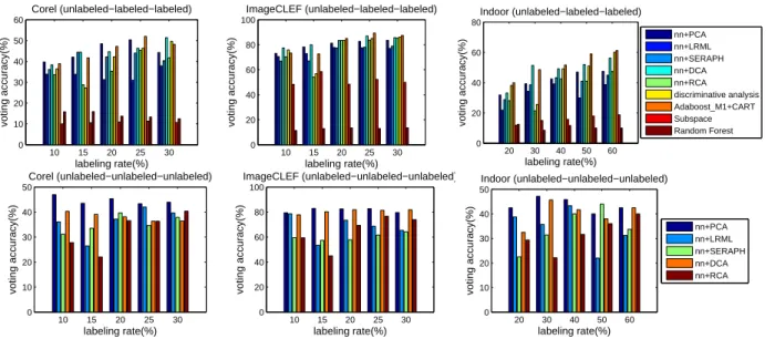
10 15 20 25 30 0 10 20 30 40 50 60 labeling rate(%) voting accuracy(%) Corel (unlabeled−labeled−labeled) 10 15 20 25 30 0 20 40 60 80 100 labeling rate(%) voting accuracy(%) ImageCLEF (unlabeled−labeled−labeled) 20 30 40 50 60 0 20 40 60 80 labeling rate(%) voting accuracy(%) Indoor (unlabeled−labeled−labeled) nn+PCA nn+LRML nn+SERAPH nn+DCA nn+RCA discriminative analysis Adaboost_M1+CART Subspace Random Forest 10 15 20 25 30 0 10 20 30 40 50 labeling rate(%) voting accuracy(%) Corel (unlabeled−unlabeled−unlabeled) 10 15 20 25 30 0 20 40 60 80 100 labeling rate(%) voting accuracy(%) ImageCLEF (unlabeled−unlabeled−unlabeled) 20 30 40 50 60 0 10 20 30 40 50 labeling rate(%) voting accuracy(%) Indoor (unlabeled−unlabeled−unlabeled) nn+PCA nn+LRML nn+SERAPH nn+DCA nn+RCA
Fig. 5. Performance comparison of different methods on three datasets with varying labeling rates.
10 15 20 25 30 0 10 20 30 40 50 labeling rate(%) voting accuracy(%) Corel (unlabeled−labeled−labeled) 10 15 20 25 30 0 20 40 60 80 100 labeling rate(%) voting accuracy(%) ImageCLEF (unlabeled−labeled−labeled) 20 30 40 50 60 0 10 20 30 40 50 labeling rate(%) voting accuracy(%) Indoor (unlabeled−labeled−labeled) GIST PHOG GB SIFT dense−SIFT SURF LBP GLCM color 10 15 20 25 30 0 10 20 30 40 50 60 labeling rate(%) voting accuracy(%) Corel (unlabeled−unlabeled−unlabeled) 10 15 20 25 30 0 20 40 60 80 100 labeling rate(%) voting accuracy(%) ImageCLEF (unlabeled−unlabeled−unlabeled) 20 30 40 50 60 0 10 20 30 40 50 labeling rate(%) voting accuracy(%) Indoor (unlabeled−unlabeled−unlabeled) GIST PHOG GB SIFT dense−SIFT SURF LBP GLCM color
Fig. 6. Performance comparison of nine different features on three datasets with varying labeling rates.
it on the validation set. For DML-eig, we tune the parameter
kin kNN from 1 to the number of the labeled training images per class minus one. All these intervals are chosen as in their released source codes. As for HDS, we use the trained network due to the limited number of labeled images.
B. Performance Analysis
In this section, we conduct a series of experiments on feature selection, classifier and feature analysis, classifier selection, sample selection as well as performance comparisons between the proposed method and other methods.
1) Feature Selection: We compare MCFS [26] with
P-CA, Laplacian score (LS) [48], discriminative least squares regression (DLSR) [49], CfsSubetEval + GreedyStepwise (CSE+GS) and the original ones (i.e. without feature se-lection). The feature selection methods select the dimension
d= 10,20, . . . ,100,120, . . . ,200 (15 sets), except CSE+GS,
which can search the optimal number automatically. We per-formk-means with the selected features for clustering and use the normalized mutual information (NMI) for evaluation.
Fig. 4 shows the plots of clustering performance versus the number of selected dimensions. In general, PCA offers performance comparable with the original features without performing feature selection. It is clear that MCFS performs well in most cases, while CSE+GS has a poor performance due to the lack of supervision information. It can be seen that MCFS significantly outperforms the original ones with SIFT features. This can be attribute to its strong ability in selecting discriminative information in high-dimensional feature spaces.
2) Classifier and Feature Analysis: Fig. 5 shows the voting
accuracy of each classifier versus the labeling rate, which represents the proportion of labeled images in the training set. For unlabeled-labeled-labeled triplets, it is clear that the per-formance of the subspace and random forest is lower than that
TABLE III
THE PERFORMANCE COMPARISON IN TERMS OF MAP (9AND10TYPES OF FEATURES)AND TIME COST(10TYPES OF FEATURES)ONCOREL DATASET
WITH LABELING RATE EQUALS TO10%, 15%, 20%, 25%AND30%. HDSUSESDCNNFEATURE EXTRATED BY ITSELF. THE BEST AND THE SECOND
BEST RESULTS ARE SHOWN IN BOLD AND UNDERLINED,RESPECTIVELY
Labeling Rate Metric SSOMKS SSOMKS SSOMKS OMKS Euclidean DCA LRML SERAPH OASIS ITML EMR DML-eig HDS
-max -max+margin -margin
10% mAP-9 0.1589 0.1597 0.1604 0.1378 0.0427 0.1284 0.1078 0.0626 0.0280 0.0413 0.0419 0.0579 mAP-10 0.3883 0.3881 0.3886 0.3837 0.0855 0.2011 0.1413 0.2997 0.2618 0.3166 0.0529 0.0255 0.4368 time(s) 99.77 97.90 98.15 67.38 0.40 0.60 2.96 3.02 21.68 336.46 0.41 1.04 15% mAP-9 0.1541 0.1535 0.1541 0.1374 0.0427 0.1320 0.1065 0.0576 0.0428 0.0697 0.0419 0.0486 mAP-10 0.3924 0.3924 0.3924 0.3872 0.0855 0.2842 0.1368 0.3078 0.2732 0.2773 0.0529 0.0799 0.4401 time(s) 377.80 377.80 377.80 137.78 0.52 0.61 3.06 3.07 26.80 311.47 0.43 2.24 20% mAP-9 0.1561 0.1561 0.1571 0.1452 0.0427 0.1280 0.0965 0.0600 0.0389 0.0424 0.0419 0.0638 mAP-10 0.3980 0.3980 0.3980 0.3915 0.0855 0.3093 0.1354 0.3093 0.3071 0.2516 0.0529 0.2042 0.4435 time(s) 1330.55 1330.55 1289.27 522.66 0.34 0.88 4.56 2.14 144.84 274.28 0.43 4.42 25% mAP-9 0.1628 0.1624 0.1642 0.1535 0.0427 0.1274 0.0860 0.0602 0.0565 0.0426 0.0419 0.0651 mAP-10 0.4032 0.4032 0.4032 0.3986 0.0855 0.3054 0.1406 0.3128 0.3044 0.2582 0.0529 0.2602 0.4470 time(s) 3892.07 3892.07 3892.07 1787.16 0.45 0.59 2.89 1.98 22.18 373.87 0.37 6.86 30% mAP-9 0.1665 0.1651 0.1644 0.1607 0.0427 0.1287 0.0882 0.0427 0.0429 0.0654 0.0419 0.0658 mAP-10 0.4102 0.4102 0.4102 0.3978 0.0855 0.3077 0.1402 0.3116 0.3116 0.2553 0.0529 0.2359 0.4513 time(s) 8789.79 8164.26 8164.26 5443.61 0.41 0.59 2.94 1.74 22.21 377.62 0.41 10.24 average rank mAP-9 1.8 2.2 1.4 3.6 9.4 4.6 5.6 7.8 10 9 10.8 7.2 mAP-10 1.2 1.4 1 2.4 8.6 4.6 7.6 3.6 5 5.4 9.8 7.8 – time 10.4 9.8 9.8 8.4 1.4 2.8 5 4.6 6.8 8.8 1.4 4.8
of other classifiers. In contrast, nn+DCA and Adaboost M1 + CART consistently exhibit significant advantages, which is partly due to the utilization of supervision information as well as error adaptive adjustment.
Fig. 6 shows the voting accuracy of each feature versus the labeling rate. It can be observed that the performance for each specific feature is data dependent. For instance, the color histogram outperforms almost all the other features on the Corel dataset, however, it has poor performance on other datasets, which is caused by the single color of the background (i.e. the sunrise is golden, the sky is blue and so on) in Corel. In contrast, as a kind of local features, SIFT is more sensitive to subtle variation in the complex scene, thus having excellent performance on the ImageCLEF and Indoor datasets.
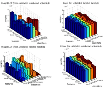
nn+DCAnn+PCA nn+LRMLnn+SERAPH nn+RCA GIST PHOG GB SIFT dense−SIFT SURF LBP GLCM color 0 2 4 6 x 10⁻³ classifiers ImageCLEF (near, unlabeled−unlabeled−unlabeled)
features weights Adaboost_M1DCA PCALRML RCASERAPH GIST PHOG GB SIFT dense−SIFT SURF LBP GLCM color 0 2 4 6 8 x 10⁻³ classifiers Corel (far, unlabeled−labeled−labeled)
features
weights
nn+PCAnn+LRML discriminative analysisnn+DCAnn+RCA
nn+SERAPHAdaboost_M1 SubspaceRandom Forest GIST PHOG GBSIFT dense−SIFT SURFLBP GLCM color 0 2 4 6 x 10⁻³ classifiers ImageCLEF (near, unlabeled−labeled−labeled)
features weights DCAPCA LRMLRCA SERAPH GIST PHOG GB SIFT dense−SIFT SURF LBP GLCM color 0 2 4 6 8 x 10⁻³ classifiers Indoor (far, unlabeled−unlabeled−unlabeled)
features
weights
Fig. 7. The obtained weights by different features and classifiers.
We learn the weight of each feature-classifier pair by min-imizing (13), and then report the results in Fig. 7. Generally
speaking, it is much easier for the feature-classifier pairs to find the farthest class than the correct class. Therefore, we may observe that these pairs get comparative weights in searching the farthest class. Intuitively, pairs having better performance receive larger weights. We can see that on the ImageCLEF dataset, the weights of Adaboost M1 + CART and nn+DCA are much larger, while those of subspace and random forests are close to zero in terms of unlabeled-labeled-labeled triplets, which is consistent with the results in Fig. 5.
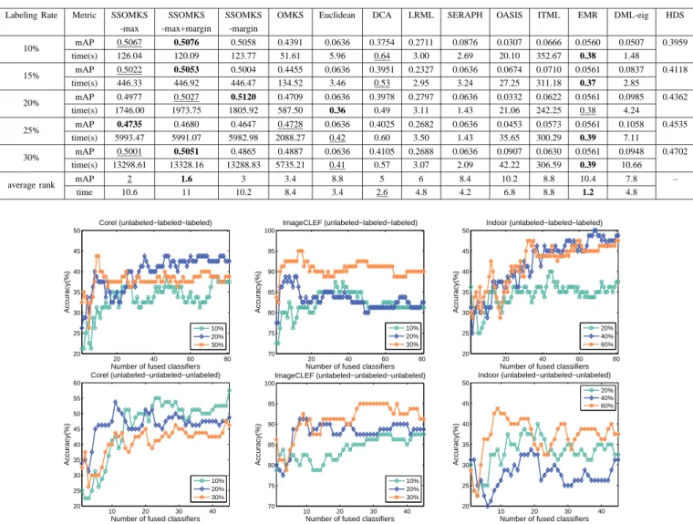
3) Selective Ensemble Learning Analysis: The process of
selective ensemble with different labeling rates is shown in Fig. 8. Intuitively, it is not necessary to exploit all the classifiers for achieving the optimal performance because a part of them may not be necessary. For unlabeled-labeled-labeled triplets, the required number of classifiers is closely related to the complexity of the scene. For instance, the best performance can be obtained with fewer than 50 base classifiers on the Corel and ImageCLEF datasets. However, due to the complicated background in the Indoor dataset, almost all the classifiers are needed when the labeling rate equals 20%. In general, for a certain dataset, the optimal number of fused classifiers decreases with the increase in the labeling rate.
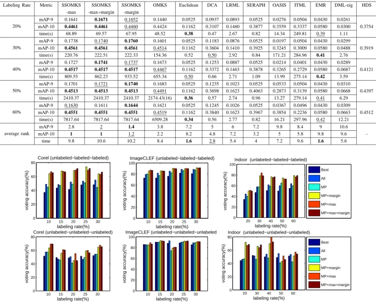
4) Sample Selection Evaluation: Fig. 9 summarizes the
performance comparison of different strategies. On the whole, the introduction of sample selection significantly improves the performance. Commonly, voting achieves a higher accuracy than using the best one. As the distribution of the decision-making on the test and validation set may differ, MP does not always outperform using all the samples. The performance of a certain strategy is data dependent. For instance, as for unlabeled-unlabeled-unlabeled triplets, MP+max performs better than MP+margin on the Corel dataset when the labeling rate is 10%, while the latter performs better on the Indoor dataset when the labeling rate is 20%.
TABLE IV
THE PERFORMANCE COMPARISON IN TERMS OF MAP (9TYPES OF FEATURES)AND TIME COST(9TYPES OF FEATURES)ONIMAGECLEFDATASET WITH
LABELING RATE EQUALS TO10%, 15%, 20%, 25%AND30%. HDSUSESDCNNFEATURE EXTRATED BY ITSELF. THE BEST AND THE SECOND BEST
RESULTS ARE SHOWN IN BOLD AND UNDERLINED,RESPECTIVELY
Labeling Rate Metric SSOMKS SSOMKS SSOMKS OMKS Euclidean DCA LRML SERAPH OASIS ITML EMR DML-eig HDS -max -max+margin -margin
10% mAP 0.5067 0.5076 0.5058 0.4391 0.0636 0.3754 0.2711 0.0876 0.0307 0.0666 0.0560 0.0507 0.3959 time(s) 126.04 120.09 123.77 51.61 5.96 0.64 3.00 2.69 20.10 352.67 0.38 1.48 15% mAP 0.5022 0.5053 0.5004 0.4455 0.0636 0.3951 0.2327 0.0636 0.0674 0.0710 0.0561 0.0837 0.4118 time(s) 446.33 446.92 446.47 134.52 3.46 0.53 2.95 3.24 27.25 311.18 0.37 2.85 20% mAP 0.4977 0.5027 0.5120 0.4709 0.0636 0.3978 0.2797 0.0636 0.0332 0.0622 0.0561 0.0985 0.4362 time(s) 1746.00 1973.75 1805.92 587.50 0.36 0.49 3.11 1.43 21.06 242.25 0.38 4.24 25% mAP 0.4735 0.4680 0.4647 0.4728 0.0636 0.4025 0.2682 0.0636 0.0453 0.0573 0.0561 0.1058 0.4535 time(s) 5993.47 5991.07 5982.98 2088.27 0.42 0.60 3.50 1.43 35.65 300.29 0.39 7.11 30% mAP 0.5001 0.5051 0.4865 0.4887 0.0636 0.4105 0.2688 0.0636 0.0907 0.0630 0.0561 0.0948 0.4702 time(s) 13298.61 13328.16 13288.83 5735.21 0.41 0.57 3.07 2.09 42.22 306.59 0.39 10.66
average rank mAP 2 1.6 3 3.4 8.8 5 6 8.4 10.2 8.8 10.4 7.8 –
time 10.6 11 10.2 8.4 3.4 2.6 4.8 4.2 6.8 8.8 1.2 4.8 20 40 60 80 20 25 30 35 40 45 50
Number of fused classifiers
Accuracy(%) Corel (unlabeled−labeled−labeled) 10% 20% 30% 20 40 60 80 70 75 80 85 90 95 100
Number of fused classifiers
Accuracy(%) ImageCLEF (unlabeled−labeled−labeled) 10% 20% 30% 20 40 60 80 20 25 30 35 40 45 50
Number of fused classifiers
Accuracy(%) Indoor (unlabeled−labeled−labeled) 20% 40% 60% 10 20 30 40 20 25 30 35 40 45 50 55 60
Number of fused classifiers
Accuracy(%) Corel (unlabeled−unlabeled−unlabeled) 10% 20% 30% 10 20 30 40 70 75 80 85 90 95 100
Number of fused classifiers
Accuracy(%) ImageCLEF (unlabeled−unlabeled−unlabeled) 10% 20% 30% 10 20 30 40 20 25 30 35 40 45 50
Number of fused classifiers
Accuracy(%)
Indoor (unlabeled−unlabeled−unlabeled)
20% 40% 60%
Fig. 8. The performance comparison in terms of classification accuracy versus the number of fused classifiers.
The classification accuracy under a much smaller training ratio is listed in Table II. It is clear that the performance is still acceptable with a relatively small training ratio, especially when sample selection is adopted. The performance is also data-dependent. In particular, a higher accuracy is obtained for ImageCLEF, which is a gray medical dataset having simpler background structure.
5) Performance Comparisons: Tables III-VI summarize the
comparison results on the nine datasets, where mAP-9 means mAP with 9 kinds of features, while mAP-10 means adopting DCNN feature as well. Tables III-V imply that SSOMKS significantly outperforms other algorithms with 9 features, while as the labeling rate increases, the supervised algorithm DCA gradually shows its superiority. In the beginning, S-SOMKS improves the most, around 15% over the OMKS. With the increase in labeling rate, the improvement decreases. Comparing mAP-9 with mAP-10, it is clear that the utilization of DCNN feature obtains significant improvement. In fact, the performance differences become smaller with better image
representation. From Table VI, the deep learning method HDS does not reveal superiority in that the generalization capability is limited without parameter tuning. In terms of computational efficiency, the Euclidean metric takes the least time. Owing to the massive triplets production as well as the time-consuming multiple kernel learning, the time cost of OMKS/SSOMKS grows rapidly as the labeling rate increases, whereas the test process only takes a few seconds. Several techniques such as distributed parallel learning [50] and mini-batch processing [51] could be applied to further reduce the time cost. Furthermore, as 50% is a relatively high ratio, we can also reduce the proportion of the training set. The average ranks of mAP demonstrate that our proposed method outperforms most of the baseline methods.
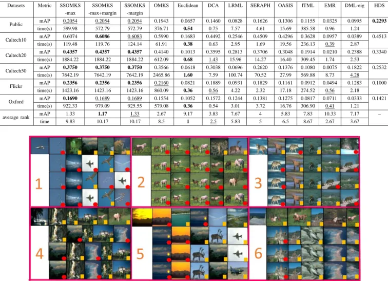
Finally, we randomly pick up several query images and compare the top 5 ranked images retrieved with different metric learning algorithms. Fig. 10 shows the qualitative comparisons of six distinct queries obtained by four diverse al-gorithms, including OMKS, SSOMKS-max, SSOMKS-margin
TABLE V
THE PERFORMANCE COMPARISON IN TERMS OF MAP (9AND10TYPES OF FEATURES)AND TIME COST(10TYPES OF FEATURES)ONINDOOR DATASET
WITH LABELING RATE EQUALS TO20%, 30%, 40%, 50%AND60%. HDSUSESDCNNFEATURE EXTRATED BY ITSELF. THE BEST AND THE SECOND
BEST RESULTS ARE SHOWN IN BOLD AND UNDERLINED,RESPECTIVELY
Labeling Rate Metric SSOMKS SSOMKS SSOMKS OMKS Euclidean DCA LRML SERAPH OASIS ITML EMR DML-eig HDS
-max -max+margin -margin
20% mAP-9 0.1641 0.1671 0.1652 0.1440 0.0525 0.0937 0.0893 0.0525 0.0276 0.0504 0.0430 0.0261 mAP-10 0.4461 0.4461 0.4460 0.4424 0.1162 0.3107 0.1460 0.3877 0.3559 0.3337 0.0580 0.0300 0.3754 time(s) 68.89 69.57 67.95 48.52 0.38 0.47 2.67 0.82 14.34 249.81 0.39 1.11 30% mAP-9 0.1738 0.1740 0.1760 0.1601 0.0525 0.1183 0.0876 0.0525 0.0197 0.0504 0.0430 0.0299 mAP-10 0.4561 0.4561 0.4561 0.4514 0.1162 0.3604 0.1410 0.3925 0.3245 0.3009 0.0580 0.0488 0.3919 time(s) 220.76 222.51 222.33 154.36 0.52 0.50 2.92 0.84 171.21 284.96 0.41 2.76 40% mAP-9 0.1727 0.1741 0.1737 0.1673 0.0525 0.1253 0.0887 0.0525 0.0214 0.0401 0.0430 0.0289 mAP-10 0.4517 0.4517 0.4517 0.4467 0.1162 0.3372 0.1463 0.3878 0.3265 0.2729 0.0580 0.0687 0.4121 time(s) 809.55 862.23 933.52 655.34 0.50 0.66 2.71 1.09 13.99 275.14 0.42 3.59 50% mAP-9 0.1701 0.1721 0.1740 0.1683 0.0525 0.1235 0.1023 0.0525 0.0533 0.0504 0.0430 0.0310 mAP-10 0.4513 0.4513 0.4513 0.4491 0.1162 0.3698 0.1623 0.4063 0.2873 0.3139 0.0580 0.0668 0.4397 time(s) 2410.37 2410.37 2410.37 2174.43(16) 0.36 0.57 2.74 0.96 13.27 279.14 0.41 6.29 60% mAP-9 0.1630 0.1611 0.1644 0.1621 0.0525 0.1245 0.1026 0.0525 0.0367 0.0496 0.0430 0.0309 mAP-10 0.4551 0.4551 0.4551 0.4519 0.1162 0.3840 0.1623 0.3967 0.3854 0.2236 0.0580 0.0663 0.4512 time(s) 7817.64 7817.64 7817.64 6509.28 0.34 0.56 2.77 0.82 16.21 297.96 0.42 12.21 average rank mAP-9 2.8 2 1.4 3.8 7.2 5 6 7.2 9.8 8.4 9 10.6 mAP-10 1 1 1.2 2.2 8.2 4.8 7.2 3.2 5 5.8 9.8 9.6 – time 9.8 10.6 10.2 8.4 1.6 2.8 5.4 4 7.2 9.6 1.6 5.6 10 15 20 25 30 0 20 40 60 80 labeling rate(%) voting accuracy(%) Corel (unlabeled−labeled−labeled) 10 15 20 25 30 0 20 40 60 80 100 labeling rate(%) voting accuracy(%) ImageCLEF (unlabeled−labeled−labeled) 20 30 40 50 60 0 20 40 60 80 100 labeling rate(%) voting accuracy(%) Indoor (unlabeled−labeled−labeled) Best All MP MP+margin MP+max MP+max+margin 10 15 20 25 30 0 20 40 60 80 labeling rate(%) voting accuracy(%) Corel (unlabeled−unlabeled−unlabeled) 10 15 20 25 30 0 20 40 60 80 100 labeling rate(%) voting accuracy(%) ImageCLEF (unlabeled−unlabeled−unlabeled) 20 30 40 50 60 0 20 40 60 80 labeling rate(%) voting accuracy(%) Indoor (unlabeled−unlabeled−unlabeled) Best All MP MP+margin MP+max MP+max+margin
Fig. 9. The performance comparison of six different strategies in terms of classification accuracy with different labeling rates on three datasets.
and SSOMKS-max+margin. From the visual results, it can be observed that SSOMKS retrieves more relevant images than OMKS. For example, for query 1, SSOMKS obtains 4 relevant images, while OMKS only obtains 1. For query 2, SSOMKS obtains the entire relevant images, while OMKS only obtains 3. Overall, SSOMKS outperforms OMKS in image retrieval due to the utilization of unlabeled images.
V. CONCLUSIONS AND FUTURE WORK
We have presented a semi-supervised online multi-kernel similarity (SSOMKS) learning framework to learn a local metric in image retrieval when the supervision information is limited. We have focused on the use of supervision information to estimate the labels of the unlabeled images. The main new aspect of our work lies in the use of classification confidence to evaluate the labeling process and select the reliably labeled
images to train the metric function. Experiments with real-world tasks have shown the effectiveness of the proposed method.
Our work is different from the current trend that encourages learning a globally linear metric and focuses on fully super-vised kernel similarity learning. Based on the characteristics in visual tasks, we have analyzed why it is necessary to introduce unlabeled images to metric learning. We have proposed a new method for reliable triplet generation, and also designed a criterion for triplet selection to improve the accuracy and efficiency in similarity learning. The proposed method for triplet generation could also be used in other algorithms that take triplets as their inputs.
Although online approaches are more scalable than the batch processing techniques, they suffer from high compu-tational cost in projections. To further improve the efficiency,
TABLE VI
THE PERFORMANCE COMPARISON IN TERMS OF MAP (10TYPES OF FEATURES)AND TIME COST(10TYPES OF FEATURES)ONPUBLIC, CALTECH10,
CALTECH20, CALTECH50, FLICKR,ANDOXFORD DATASETS,RESPECTIVELY. HDSUSESDCNNFEATURE EXTRATED BY ITSELF. THE BEST AND THE
SECOND BEST RESULTS ARE SHOWN IN BOLD AND UNDERLINED,RESPECTIVELY
Datasets Metric SSOMKS SSOMKS SSOMKS OMKS Euclidean DCA LRML SERAPH OASIS ITML EMR DML-eig HDS -max -max+margin -margin
Public mAP 0.2054 0.2054 0.2054 0.1943 0.0657 0.1460 0.0828 0.1626 0.1306 0.1155 0.0325 0.0995 0.2293 time(s) 599.98 572.79 572.79 376.71 0.54 0.75 7.57 4.61 15.69 385.58 0.96 1.24 Caltech10 mAP 0.6074 0.6086 0.6083 0.5990 0.1683 0.4492 0.2546 0.4509 0.4296 0.3628 0.0957 0.0389 0.4513 time(s) 119.48 119.76 124.14 61.91 0.38 0.63 2.95 1.69 19.56 236.13 0.39 2.87 Caltech20 mAP 0.4357 0.4357 0.4357 0.4140 0.1013 0.3595 0.2813 0.3706 0.3048 0.1914 0.0210 0.2388 0.3340 time(s) 1884.22 1884.22 1884.22 612.09 0.68 1.43 15.96 14.27 16.40 309.45 1.74 2.53 Caltech50 mAP 0.3750 0.3750 0.3750 0.3566 0.0618 0.3038 0.0696 0.2620 0.1376 0.1080 0.0075 0.1822 0.2532 time(s) 7642.19 7642.19 7642.19 2465.86 1.60 7.59 100.74 70.52 27.99 569.88 8.73 4.28 Flickr mAP 0.2356 0.2356 0.2356 0.2160 0.0821 0.1889 0.0931 0.1829 0.1161 0.0912 0.0494 0.1283 0.1000 time(s) 1423.16 1423.16 1423.16 860.09 0.36 0.56 4.22 2.32 17.18 274.52 0.56 2.18 Oxford mAP 0.1690 0.1689 0.1689 0.1554 0.1052 0.1572 0.1244 0.1381 0.1275 0.0817 0.0711 0.0333 0.1421 time(s) 922.33 979.09 925.55 579.08 0.36 0.54 3.01 3.72 16.76 306.90 0.41 1.21
average rank mAP 1.33 1.17 1.33 2.67 9.17 3.83 7.67 4 5.83 7.83 10.33 7.17 –
time 9.83 10.17 10.17 8.5 1 2.5 5.83 5 6.5 8.67 2.67 3.67
Fig. 10. Qualitative comparison of image similarity search results on the Corel data set by different algorithms. For each block, the first image is the query, and the results from the first line to the fourth line represents OMKS, SSOMKS-max, SSOMKS-margin and SSOMKS-max+margin, respectively. The ground truth for the queries are as follows: 1 (sky, jet, plane), 2 (field, horses, mare, foals), 3 (tails, snow, coyote, light), 4 (water, tree, ships, sunset), 5 (mountain, sun, clouds, tree), 6 (sky, water, monument). The dots in red represent the images of the same semantic theme with the queries, and squares in yellow represent the images from different semantic themes.
reducing the number of projections and performing distributed learning could be considered. In the future, we will explore the potentials of the techniques such as mini-batch and adaptive sampling for computationally efficient metric learning.
ACKNOWLEDGMENT
We wish to thank the associate editor and the anonymous reviewers for their contributions to improving the quality of this paper.
REFERENCES
[1] M. S. Lew, N. Sebe, C. Djeraba, and R. Jain, “Content-based multimedia information retrieval: State of the art and challenges,” ACM Trans. Multi.
Comput. Commun. Appl., vol. 2, no. 1, pp. 1–19, 2006.
[2] Y. Jing and S. Baluja, “Visualrank: Applying pagerank to large-scale image search,” IEEE Trans. Pattern Anal. Mach. Intell., vol. 30, no. 11, pp. 1877–1890, 2008.
[3] N. Jiang, W. Liu, and Y. Wu, “Order determination and sparsity-regularized metric learning adaptive visual tracking,” in Proc. IEEE
Conf. Comput. Vis. Pattern Recog. IEEE, 2012, pp. 1956–1963. [4] E. P. Xing, A. Y. Ng, M. I. Jordan, and S. Russell, “Distance metric
learning with application to clustering with side-information,” Adv.
Neural Inf. Process. Syst., vol. 15, pp. 505–512, 2003.
[5] A. Bellet, A. Habrard, and M. Sebban, “A survey on metric learning for feature vectors and structured data,” arXiv preprint arXiv:1306.6709, 2013.
[6] A. Bar-Hillel, T. Hertz, N. Shental, and D. Weinshall, “Learning distance functions using equivalence relations,” in Proc. 20th Int. Conf. on Mach.
Learn., vol. 3, 2003, pp. 11–18.
[7] J. V. Davis, B. Kulis, P. Jain, S. Sra, and I. S. Dhillon, “Information-theoretic metric learning,” in Proc. 24th Int. Conf. on Mach. Learn. ACM, 2007, pp. 209–216.
[8] K. Q. Weinberger and L. K. Saul, “Distance metric learning for large margin nearest neighbor classification,” J. Mach. Learn. Res., vol. 10, no. Feb, pp. 207–244, 2009.
[9] S. C. Hoi, W. Liu, and S.-F. Chang, “Semi-supervised distance metric learning for collaborative image retrieval and clustering,” ACM Trans.
Multi. Comput. Commun. Appl., vol. 6, no. 3, p. 18, 2010.
in Proc. 33rd Int. Conf. on Mach. Learn., 2016.
[11] P. Jain, B. Kulis, J. V. Davis, and I. S. Dhillon, “Metric and kernel learning using a linear transformation,” J. Mach. Learn. Res., vol. 13, no. Mar, pp. 519–547, 2012.
[12] J. Wang, A. Kalousis, and A. Woznica, “Parametric local metric learning for nearest neighbor classification,” in Adv. Neural Inf. Process. Syst., 2012, pp. 1601–1609.
[13] J. Wang, K. Sun, F. Sha, S. Marchand-Maillet, and A. Kalousis, “Two-stage metric learning.” in Proc. 31st Int. Conf. on Mach. Learn., 2014, pp. 370–378.
[14] L. Cheng, “Riemannian similarity learning.” in Proc. 30th Int. Conf. on
Mach. Learn., 2013, pp. 540–548.
[15] G. Niu, B. Dai, M. Yamada, and M. Sugiyama, “Information-theoretic semi-supervised metric learning via entropy regularization,” Neural
computation, vol. 26, no. 8, pp. 1717–1762, 2014.
[16] Y. Ying and P. Li, “Distance metric learning with eigenvalue optimiza-tion,” J. Mach. Learn. Res., vol. 13, no. Jan, pp. 1–26, 2012. [17] B. McFee and G. Lanckriet, “Learning multi-modal similarity,” J. Mach.
Learn. Res., vol. 12, no. Feb, pp. 491–523, 2011.
[18] P. Xie and E. P. Xing, “Multi-modal distance metric learning,” in Proc.
23rd Int. Joint Conf. Artificial Intelligence, 2013, pp. 1806–1812.
[19] X. Lu, Y. Wang, X. Zhou, and Z. Ling, “A method for metric learning with multiple-kernel embedding,” Neural Processing Letters, vol. 43, no. 3, pp. 905–921, 2016.
[20] C. Xu, D. Tao, and C. Xu, “Multi-view intact space learning,” IEEE
Trans. Pattern Anal. Mach. Intell., vol. 37, no. 12, pp. 2531–2544, 2015.
[21] P. Wu, S. C. Hoi, H. Xia, P. Zhao, D. Wang, and C. Miao, “Online multimodal deep similarity learning with application to image retrieval,” in Proc. 21st Int. Conf. Multimedia. ACM, 2013, pp. 153–162. [22] P. Wu, S. C. Hoi, P. Zhao, C. Miao, and Z.-Y. Liu, “Online multi-modal
distance metric learning with application to image retrieval,” IEEE Trans.
Knowl. Data Eng., vol. 28, no. 2, pp. 454–467, 2016.
[23] H. Xia, S. C. Hoi, R. Jin, and P. Zhao, “Online multiple kernel similarity learning for visual search,” IEEE Trans. Pattern Anal. Mach. Intell., vol. 36, no. 3, pp. 536–549, 2014.
[24] Z.-J. Zha, T. Mei, M. Wang, Z. Wang, and X.-S. Hua, “Robust distance metric learning with auxiliary knowledge.” in Proc. 21st Int. Joint Conf.
Artificial Intelligence, 2009, pp. 1327–1332.
[25] G. Kunapuli and J. Shavlik, “Mirror descent for metric learning: A unified approach,” in Proc. Eur. Conf. Mach. Learn. Knowl. Disc.
Databases. Springer, 2012, pp. 859–874.
[26] D. Cai, C. Zhang, and X. He, “Unsupervised feature selection for multi-cluster data,” in Proc. 16th ACM SIGKDD Int. Conf. Knowl. Discovery
Data Mining. ACM, 2010, pp. 333–342.
[27] M. Belkin and P. Niyogi, “Laplacian eigenmaps and spectral techniques for embedding and clustering.” in Adv. Neural Inf. Process. Syst., vol. 14, 2001, pp. 585–591.
[28] B. Efron, T. Hastie, I. Johnstone, R. Tibshirani et al., “Least angle regression,” Ann. Stat., vol. 32, no. 2, pp. 407–499, 2004.
[29] T. Liu, D. Tao, M. Song, and S. Maybank, “Algorithm-dependent generalization bounds for multi-task learning,” IEEE Trans. Pattern
Anal. Mach. Intell., 2016.
[30] Z.-H. Zhou, J. Wu, and W. Tang, “Ensembling neural networks: many could be better than all,” Artif. Intell., vol. 137, no. 1, pp. 239–263, 2002.
[31] L. Li, Q. Hu, X. Wu, and D. Yu, “Exploration of classification confidence in ensemble learning,” Pattern Recog., vol. 47, no. 9, pp. 3120–3131, 2014.
[32] T. Van Gestel, J. A. Suykens, B. Baesens, S. Viaene, J. Vanthienen, G. Dedene, B. De Moor, and J. Vandewalle, “Benchmarking least squares support vector machine classifiers,” Mach. Learn., vol. 54, no. 1, pp. 5–32, 2004.
[33] J. Liu, S. Ji, J. Ye et al., “Slep: Sparse learning with efficient projec-tions,” Arizona State University, vol. 6, p. 491, 2009.
[34] V. Vapnik, Estimation of dependences based on empirical data. Springer Science & Business Media, 2006.
[35] L. Xu, J. Neufeld, B. Larson, and D. Schuurmans, “Maximum margin clustering,” in Adv. Neural Inf. Process. Syst., 2004, pp. 1537–1544. [36] D. Tao, X. Tang, X. Li, and X. Wu, “Asymmetric bagging and random
subspace for support vector machines-based relevance feedback in image retrieval,” IEEE Trans. Pattern Anal. Mach. Intell., vol. 28, no. 7, pp. 1088–1099, 2006.
[37] C. Xu, D. Tao, and C. Xu, “Large-margin multi-view information bottleneck,” IEEE Trans. Pattern Anal. Mach. Intell., vol. 36, no. 8, pp. 1559–1572, 2014.
[38] H. Ahn, H. Moon, M. J. Fazzari, N. Lim, J. J. Chen, and R. L. Kodell, “Classification by ensembles from random partitions of
high-dimensional data,” Comput. Stat. Data Anal., vol. 51, no. 12, pp. 6166– 6179, 2007.
[39] L. Lam and S. Suen, “Application of majority voting to pattern recog-nition: an analysis of its behavior and performance,” IEEE Trans. Syst.
Man Cybern., vol. 27, no. 5, pp. 553–568, 1997.
[40] S. C. Hoi, W. Liu, M. R. Lyu, and W.-Y. Ma, “Learning distance metrics with contextual constraints for image retrieval,” in Proc. IEEE Conf.
Comput. Vis. Pattern Recog., vol. 2. IEEE, 2006, pp. 2072–2078. [41] Y. Freund, R. E. Schapire et al., “Experiments with a new boosting
algorithm,” in Proc. 13th Int. Conf. on Mach. Learn., vol. 96, 1996, pp. 148–156.
[42] L. Breiman, J. Friedman, C. J. Stone, and R. A. Olshen, Classification
and regression trees. CRC press, 1984.
[43] C. R. Rao, “The utilization of multiple measurements in problems of biological classification,” J. Royal Statistical Soc., vol. 10, no. 2, pp. 159–203, 1948.
[44] L. Breiman, “Random forests,” Mach. Learn., vol. 45, no. 1, pp. 5–32, 2001.
[45] G. Chechik, V. Sharma, U. Shalit, and S. Bengio, “Large scale online learning of image similarity through ranking,” J. Mach. Learn. Res., vol. 11, no. Mar, pp. 1109–1135, 2010.
[46] B. Xu, J. Bu, C. Chen, D. Cai, X. He, W. Liu, and J. Luo, “Efficient manifold ranking for image retrieval,” in Proc. 34th Int. ACM SIGIR
Conf. Research and Development in Information Retrieval. ACM, 2011,
pp. 525–534.
[47] K. Lin, H.-F. Yang, J.-H. Hsiao, and C.-S. Chen, “Deep learning of binary hash codes for fast image retrieval,” in Proc. IEEE Conf. Comput.
Vis. Pattern Recog. Workshops, 2015, pp. 27–35.
[48] X. He, D. Cai, and P. Niyogi, “Laplacian score for feature selection,” in Adv. Neural Inf. Process. Syst., 2005, pp. 507–514.
[49] S. Xiang, F. Nie, G. Meng, C. Pan, and C. Zhang, “Discriminative least squares regression for multiclass classification and feature selection,”
IEEE Trans. Neural Net. Learn. Syst., vol. 23, no. 11, pp. 1738–1754,
2012.
[50] F. Wang and J. Sun, “Survey on distance metric learning and dimen-sionality reduction in data mining,” Data. Min. Knowl. Disc., vol. 29, no. 2, pp. 534–564, 2015.
[51] Q. Qian, R. Jin, J. Yi, L. Zhang, and S. Zhu, “Efficient distance metric learning by adaptive sampling and mini-batch stochastic gradient descent (sgd),” Mach. Learn., vol. 99, no. 3, pp. 353–372, 2015.
Jianqing Liang received the B.E. degree from the School of Computer and Information Technology, Shanxi University, Taiyuan, Shanxi, China, in 2013. She is currently pursuing the Ph.D. degree with the College of Computer Science and Technology in Tianjin University. Her current research interests include metric learning, semi-supervised learning and machine learning.
Qinghua Hu received B. E., M. E. and PhD de-grees from Harbin Institute of Technology, Harbin, China in 1999, 2002 and 2008, respectively. He once worked with Harbin Institute of Technology as assistant professor and associate professor from 2006 to 2011 and a postdoctoral fellow with the Hong Kong Polytechnic University. He is now a full professor with Tianjin University. His research interests are focused on intelligent modeling, data mining, knowledge discovery for classification and regression. He is the PC co-chair of RSCTC 2010, CRSSC 2012, and ICMLC 2014 and severs as referee for a great number of journals and conferences. He has published more than 100 journal and conference papers in the areas of pattern recognition, machine learning and data mining.
Wenwu Wang received the B.Sc. degree in auto-matic control in 1997, the M.E. degree in control science and control engineering in 2000, and the Ph.D. degree in navigation guidance and control in 2002, all from Harbin Engineering University, Harbin, China.
He then joined Kings College, London, U.K., in May 2002, as a postdoctoral research associate and transferred to Cardiff University, Cardiff, U.K., in January 2004, where he worked in the area of blind signal processing. In May 2005, he joined the Tao Group Ltd. (now Antix Labs Ltd.), Reading, U.K., as a DSP engineer working on algorithm design and implementation for real-time and embedded audio and visual systems. In September 2006, he joined Creative Labs, Ltd., Egham, U.K., as an engineer, working on 3D spatial audio for mobile devices. Since May 2007, he has been with the Centre for Vision Speech and Signal Processing, University of Surrey, Guildford, U.K., where he is currently a Reader in Signal Processing, and a Co-Director of the Machine Audition Lab. He is a member of the Ministry of Defence (MoD) University Defence Research Collaboration (UDRC) in Signal Processing (since 2009), a member of the BBC Audio Research Partnership (since 2011), an associate member of Surrey Centre for Cyber Security (since 2014), and a member of the MRC/EPSRC Microphone Network (since 2015). During spring 2008, he has been a visiting scholar at the Perception and Neurodynamics Lab and the Center for Cognitive Science, The Ohio State University.
His current research interests include blind signal processing, sparse signal processing, audio-visual signal processing, machine learning and perception, machine audition (listening), and statistical anomaly detection. He has (co)-authored over 150 publications in these areas, including two books Machine Audition: Principles, Algorithms and Systems (IGI Global, 2010) and Blind Source Separation: Advances in Theory, Algorithms and Applications (Springer, 2014). He is currently an Associate Editor for IEEE TRANSACTIONS ON SIGNAL PROCESSING. He is also Publication Co-Chair of ICASSP 2019 (to be held in Brighton, UK). He was a Tutorial Speaker on ICASSP 2013, UDRC Summer School 2014, 2015 and 2016, and SpaRTan/MacSeNet Spring School 2016.
Yahong Han received the Ph.D. degree from Zhe-jiang University, Hangzhou, China. He is currently an Associate Professor with the School of Computer Science and Technology, Tianjin University, Tianjin, China. His current research interests include multi-media analysis, retrieval, and machine learning.