Technology adoption and farmer efficiency in multiple crops
production in eastern Ethiopia:
A comparison of parametric and non-parametric distance functions
Arega D. Alene* and Manfred Zeller**Abstract
This study compares the empirical performances of the parametric distance functions (PDF) and data envelopment analysis (DEA) with applications to adopters of improved cereal production technology in eastern Ethiopia. The results from both approaches re-vealed substantial technical inefficiencies of production among the sample farmers. Tech-nical efficiency estimates obtained from the two approaches are positively and signifi-cantly correlated. However, the DEA approach is shown to be very sensitive to outliers as well as to the choice of orientation. The PDF results are relatively more robust. The re-sults from the preferred PDF approach revealed that adopters of improved technology have average technical efficiencies of 79%, implying that they could potentially raise their food crop production by an average 21% through full exploitation of the potentials of im-proved varieties and mineral fertilizer. The results confirm that food production even un-der improved technology involves substantial inefficiency. The paper concludes with a discussion of potential underlying factors influencing farmer efficiency under improved technology, such as poor extension, education, credit, and input supply systems.
Keywords:Multiple outputs, Distance functions, DEA, Technical efficiency, Ethiopia
Introduction
In a dynamic environment, it is argued that farmers encounter considerable ineffi-ciencies before the realization of the intended gains from technological change (Ali and Chaudhry, 1990; Ali and Byerlee, 1991; Xu and Jeffrey, 1998). In other words, there is a time lag between farmers’ adoption of a new technology and achieving efficient use of that technology. Knowledge of the extent and causes of such inefficiencies among adopters of improved technology will guide policy makers to help increase agricultural production by designing more effective and efficient institutional support services. In an effort to raise agricultural production and productivity, policy makers in developing countries have placed substantial emphasis on new production technologies and their adoption by farmers.
The development strategy of the Ethiopian government aims to ensure greater food security through increased use of improved agricultural production technologies, includ-ing fertilizer, improved seeds, chemicals, and improved cultural practices (Techane and Mulat, 1999). However, while various incentive measures have been used to induce farmers to achieve a high rate of adoption of the chosen modern technologies, little or * Arega D. Alene. International Institute of Tropical Agriculture, c/o L.W. Lambourn & Co., Carolyn
House, 26 Dingwall Road, Croydon CR9 3EE, UK.
** Manfred Zeller. Institute of Rural Development, University of Göttingen, Waldweg 26, D-37073, Göttingen, Germany.
no attention has been given to the question of whether there is appropriate application and efficient use of these technologies. This is mainly attributed to the wrong hypothe-sis that farmers may not be able to select appropriate technologies but can nevertheless operate technology efficiently when chosen for them (Kalirajan, 1991). In Ethiopia, for instance, cereal yields have not shown substantial improvement in spite of the sharp increase in the use of improved seeds, fertilizer and other inputs (Mulat, 1999).
Although it is always of interest to know the efficiency with which farmers use their resources under new technology, any evidence of farmer inefficiency could just be due to inappropriate methods used. For example, the single-output production frontier ap-proach has been the standard apap-proach to farm level efficiency analysis and most have revealed substantial inefficiencies of production in developing countries regardless of the level of education, quality of extension services, and infrastructure available in the countries studied. This approach has the limitation that it accommodates only an aggre-gate index of agricultural output (mostly using monetary values) when the reality is that farmers cultivate a range of crops with high technical interdependence in production. Parametric and non-parametric distance functions, on the other hand, accommodate multiple outputs without having to aggregate them into an index.
Farrell’s (Farrell, 1957) seminal article has led to the development of several tech-niques for the measurement of technical efficiency of production. These techtech-niques can be broadly categorized into two approaches: parametric and nonparametric. The para-metric stochastic frontier production function (SFP) approach (Aigner et al., 1977; Meeusen and van den Broeck, 1977) and the nonparametric mathematical programming approach, commonly referred to as data envelopment analysis (DEA) (Charnes et al., 1978; Färe et al., 1989; Färe et al., 1994) are the two most popular techniques used in efficiency analysis. While the majority of applied economists would be familiar with the use of production, cost and profit functions as alternative methods of describing a pro-duction technology, the additional alternatives of the (parametric) input- and output dis-tance functions (PDF) have also been available since their development by Shephard (1970). However, it is only in recent years that applications involving input and output distance functions, motivated by the desire to calculate technical efficiencies and shadow prices, have begun to appear (e.g., Färe et al., 1993; Grosskopf et al., 1997; Hailu and Veeman, 2000).
The above three approaches, namely the SFP, DEA, and PDF have their own limita-tions and strengths. While Coelli (1995) presents a review of the limitalimita-tions, strengths and applications of SFP and DEA, Coelli and Perelman (1999) point out the strengths and limitations of DEA and PDF approaches. The main strengths of the SFP approach are that it deals with stochastic noise and permits statistical tests of hypotheses pertain-ing to production structure and degree of inefficiency. The need for impospertain-ing an explicit parametric form for the underlying technology and explicit distributional assumption for the inefficiency term are the main weaknesses of this approach (Coelli, 1995; Sharma et al., 1999). The main advantages of the DEA approach are that it avoids parametric specification of technology as well as the distributional assumption for the inefficiency term. However, because DEA is deterministic and attributes all the deviations from the frontier to inefficiencies, a frontier estimated by DEA is likely to be sensitive to meas-urement errors and other noise in the data (Coelli, 1995; Coelli and Perelman, 1999). The principal advantage of the PDF approach is that it allows the possibility of specify-ing a multiple-input, multiple-output technology when price information is not available
or alternatively when price information is available but cost, profit or revenue function representations are precluded because of violations of the required behavioural assump-tions (Coelli and Perelman, 1999). However, the estimates from a stochastic distance function are not well behaved requiring that the parameters and firm-specific efficien-cies be computed either through parametric programming or corrected ordinary least squares (COLS) (Coelli and Perelman, 1996).
Given the strengths and weaknesses of the three approaches, it has been of interest to compare their empirical performance and examine the sensitivity of technical efficiency measures to the selection of analytical approach. Some studies already compared the SFP and DEA approaches (e.g., Ferrier and Lovell, 1990; Kalaitzandonakes and Dunn, 1995; Drake and Weyman-Jones, 1996; Sharma et al., 1997,1999; Wadud and White, 2000). Coelli and Perelman (1999) compared methods of estimating parametric and non-parametric distance functions. For the parametric approach, for instance, they com-pared linear programming and corrected ordinary least squares methods and both meth-ods were found to be equally appropriate.
A related interest in this study is to examine the advantages or disadvantages of im-posing a parametric form of the distance function representation of agricultural produc-tion technology relative to the parametric form. We compare parametric and non-parametric distance functions, using linear programming methods to estimate the para-metric forms and DEA to estimate the non-parapara-metric representations of distance func-tions. The main objective of this paper is, therefore, to estimate farm level technical efficiency under improved technology in eastern Ethiopia using PDF and DEA and to illustrate the sensitivity of efficiency measures to the choice of approach and orienta-tion. The remainder of this paper is organised as follows. The next section presents the analytical framework and the data, and empirical models are discussed in the third sec-tion. The results are presented and discussed in the fourth section and the last section draws conclusions.
Analytical framework
Non-parametric distance functions (or DEA)
DEA is a nonparametric approach to distance function estimation (Färe et al., 1994). The method involves the use of linear programming to construct a piecewise linear en-velopment frontier over the data points such that all observed points lie on or below the production frontier. Let X be a K N× matrix of inputs, which is constructed by plac-ing the input vectors, xi, of all N firms side by side, and Y denotes the M N× output matrix which is formed in an analogous manner.
The output oriented variable returns to scale (VRS) DEA frontier is defined by the solution to N linear programs of the form
subject to θ ,λ i i minθ y / θ Yλ 0 x Xλ 0 N1 λ 1 λ 0, - + ≥ + ≥ = ¢ ≥ (1)
where N1 is an N×1vector of 1s, λ is an N×1 vector of weights, and θ is the output distance measure (see section 2.3). We note that 0≤ ≤θ 1 and that 1/θ is the propor-tional expansion in outputs that could be achieved the ith firm, with input quantities held constant.
In a similar manner, the input-orientated VRS DEA frontier is defined by the solu-tion to N linear programs of the form
, max subject to 0 / 0 1' 1 0, i i y Y x X N ρ λ ρ λ ρ λ λ λ − + ≥ − ≥ = ≥ (2)
where ρ is the input distance measure (see section 2.3). We note that 1≤ ≤ ∞ρ and that 1/ρ is the proportional reduction in inputs that could be achieved by the ith firm, with output quantities held constant.
The technical efficiency measure under constant returns to scale (CRS), also called the ‘overall’ technical efficiency measure, is obtained by solving N linear programs of
the form CRS CRS CRS min subject to 0 0 0 i i i i i Y y x X θ θ λ θ λ λ − + ≤ − ≥ ≥ (3) where CRS i
θ is a technical efficiency measure of the ithfirm under CRS and CRS
0≤θi ≤1.
The output and input oriented models will estimate exactly the same frontier surface and, therefore, by definition, identify the same set of firms as being efficient. The effi-ciency measures may, however, differ between the input and output orientations. Under the assumption of constant returns to scale, the estimated frontier and the efficiency measures remain unaffected by the choice of orientation (Coelli and Perelman, 1999). Parametric distance functions (PDF)
Multi-output distance functions have provided a promising new solution to the sin-gle-output restriction and the implied aggregation of several outputs implicit in standard production functions. To define an output-distance function we begin by defining the production technology of the firm using the output set V x( ) which represent the set of all output vectors, ,
M
y R+∈ which can be produced using the input vector, . N x R + ∈ That is,
{
}
( ) M : can produce . V x = y R x∈ + y (4)The output distance function is then defined on the output set, V x( ), as
{
}
( , ) min :( / ) ( ) .
o
( , )
o
D x y is non-decreasing, positively linearly homogenous and convex in y, and de-creasing in x (Coelli et al., 1998). The distance function, D x yo( , ), will take a value which is less than or equal to one if the output vector, y, is an element of the feasible production set, V x( ). That is, D x yo( , ) 1≤ if y V x∈ ( ). Furthermore, the distance func-tion will take a value of unity if y is located on the outer boundary of the production possibility set. That is,
{
}
( , ) 1 if Isoq ( ) : ( ), ( ), 1 . o D x y y V x y y V x wy V x w = ∈ = ∈ ∉ >An input distance function is defined in a similar manner. However, rather than look-ing at how the output vector may be proportionally expanded with the input vector held fixed, it considers by how much the input vector may be proportionally contracted with the output vector held fixed. The input distance function may be defined on the input set, V y( ), as
( )
, max{
:( ) ( )
}
, ID x y = ρ x ρ ∈V y (6)
where the input set V y( ) represents the set of all input vectors, ,
N
x R
+
∈ which can pro-duce the output vector, .
M
y R∈ + That is,
{
}
( ) N: can produce .
V y = ∈x R x+ y (7)
The input distance function, DI
( )
x,y , will take a value which is greater than or equal to unity if the input vector, x, is an element of the feasible input set, V y( ). That is,( , ) 1 if ( ). I
D x y ≥ x V y∈ Furthermore, the distance function will take a value of unity if
x is located on the inner boundary of the input requirement set, V y( ).
Under constant returns to scale, the output distance function is the inverse of the in-put distance function (i.e., DO=1/ )DI (Färe et al., 1994). That is, the proportion by
which one is able to radially expand output (with input held fixed) will be exactly equal to the proportion by which one is able to radially reduce input usage (with output held fixed). Unlike in DEA, both the efficiency measures and the estimated frontier obtained from the output and input distance functions are different (Coelli and Perelman, 1999).
Data and empirical models
Data
The data used in this study come from a survey of a sample of 53 smallholder farm-ers who participated in the extension program in Meta district, eastern Ethiopia during the 2001/2002 cropping season. Meta district is a high potential cereal production zone given its better rainfall amount and distribution. A sampling frame of all farmers in the highland zone of Meta district who participated in the extension program was prepared and the surveyed farmers were randomly selected using simple random sampling. The sample farmers used improved maize and wheat varieties and chemical fertilizer and mainly grew maize, wheat, and barley. Data were collected through frequent visits to
the sample households’ crop fields and homes throughout the cropping season. Input data were collected on a fortnight basis by asking the farmer to recall the activities on that particular plot during the past two weeks. Labour time was disaggregated by source, gender, age, and field operation. The quantities of seed, fertilizer, pesticides, and herbicides, and the prices of all purchased inputs were also collected during this time. Output data on all the quantities of crops harvested from each plot were recorded.
Translog output and input distance functions
Input and output distance function technologies are estimated in this paper using a parametric linear programming method (also known as goal programming). This method was first applied by Aigner and Chu (1968) to estimate a single-output Cobb-Douglas frontier production function. It involves specifying a parametric form of the production technology and using linear programming (LP) to compute parameter val-ues, which provide the closest possible envelopment of the observed data. Färe et al. (1993) use a generalization of this approach to estimate a translog output distance func-tion. Such flexible functional forms provide a second order approximation to the un-known technology. The translog functional form is commonly used in distance function estimations (e.g., Färe et al., 1989; Färe et al., 1993; Coelli and Perelman, 1999; Hailu and Veeman, 2000), and was chosen to specify the empirical input and output distance function models in this study.
The translog output distance function for the case of Moutputs and Ninputs is specified as 1 0 2 ' ' 1 1 ' 1 1 1 1 ' ' 2 2 1 ' 1 1 1 ln ln ln ln ln ln ln ln ln , 1,2,..., , M M M N oi m m mm m m n n m m m n N N M N nn n n mn m n n n m n D y y y x x x y x i K α α α β β δ = = = = = = = = = + + + + + =
∑
∑∑
∑
∑∑
∑∑
(8)where DOi represents output distance; i denotes the ithfirm in the sample; n indexes inputs such that the subscripts 1,2,3, and 4 represent, respectively, land, labour, fertil-izer, and materials; mindexes outputs such that the subscripts 1,2, and 3 represent, re-spectively, maize, wheat and barley produced in kilograms. The restrictions required for homogeneity of degree +1 in outputs are
1 1, M m m α = =
∑
(9) ' ' 1 0, 1,2,..., , M mm m m M α = = =∑
(10) 1 0, 1,2,..., M mn m n N δ = = =∑
(11)and those required for symmetry are
' ' ' ' , , ' 1,2,..., , , , ' 1,2,..., . mm m m nn n n m m M n n N α α β β = = = = (12)
Values for the unknown parameters in eq.(8) are obtained from the following optimiza-tion problem 53 , , 1 Maximize ln Oi( , ) i D x y α β δ
∑
= (13)subject to the constraints that
lnDOi≤0, i=1,...,53 farms, (14) ln Oi( , ) 0, 1,...,53, 1,2,3, m D x y i m y ∂ ≥ = = ∂ (15) ln Oi( , ) 0, 1,...,53, 1,2,3,4, n D x y i n x ∂ ≤ = = ∂ (16)
along with the homogeneity and symmetry constraints defined in Eqs. (9) - (12). A translog input distance function may be estimated in a similar manner. The input dis-tance function is specified as
1 0 2 ' ' 1 1 ' 1 1 1 1 ' ' 2 2 1 ' 1 1 1 ln ln ln ln ln ln ln ln ln , 1,2,..., , M M M N Ii m m mm m m n n m m m n N N M N nn n n mn m n n n m n D y y y x x x y x i K α α α β β δ = = = = = = = = = + + + + + =
∑
∑∑
∑
∑∑
∑∑
(17)where lnDIi represents an input distance. The restrictions required for homogeneity of degree +1 in inputs are
1 1, N n n= β =
∑
(18) ' ' 1 0, 1,2,..., , N nn n n N β = = =∑
(19) 1 0, 1,2,..., N mn n m M δ = = =∑
(20)and those required for symmetry are unchanged from eq. (12).
Values for the unknown parameters in eq. (17) are obtained from the following opti-mization problem 53 , , 1 Minimize ln ( , )Ii i D x y α β δ
∑
= (21) subject to the constraints thatlnDIi≥0, i=1,2,...,53farms, (22) ln ( , ) 0, 1,...,53,Ii 1,2,3, m D x y i m y ∂ ≤ = = ∂ (23)
ln ( , ) 0, 1,...,53, 1,2,3,4,Ii n D x y i n x ∂ ≥ = = ∂ (24)
along with the homogeneity and symmetry constraints defined in eqs. (18) - (20) and eq. (12).
Constant returns to scale can be imposed upon this input distance function by impos-ing homogeneity of degree –1 in outputs. This involves the additional constraints de-fined in eq. (11) along with
1 1 M m m α = = −
∑
(25)An identical constant returns to scale technology can be obtained by imposing homoge-neity of degree –1 in inputs upon the output distance function defined earlier.
The parameter estimation for each of the input and output distance functions is car-ried out by imposing 442 equality and inequality constraints. These are 53 feasibility constraints, 371 monotonocity constraints relating to inputs (212) and outputs (159), 8 linear homogeneity conditions, and 9 translog symmetry restrictions. While the linear homogeneity and translog symmetry restrictions are equality constraints applied directly on the parameters estimated, Hailu and Veeman (2000) noted the difficulty of interpret-ing the remaininterpret-ing weak inequality restrictions in terms of gains in degrees of freedom because these constraints contribute to the estimation indirectly through restrictions on the functions of the parameters (e.g., derivatives, etc.) rather than as direct restrictions on the parameters themselves. Nonetheless, these inequality constraints are important to narrow down the parameter space and to guide the estimation so that the chosen pa-rameters locate the technology and the corresponding theoretically desirable properties are satisfied at all data points. GAMS programs were written and solved to compute the parameter estimates.
Empirical results Parameter estimates
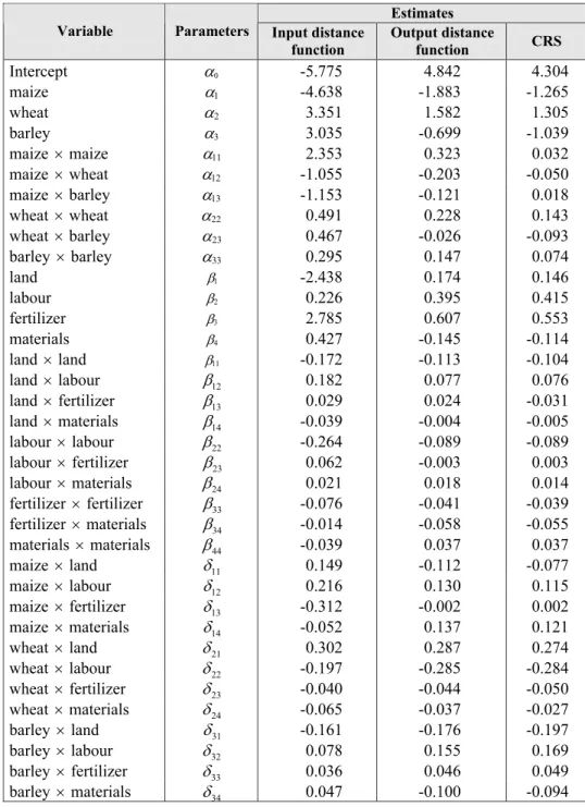
The parameter estimates of the translog input, output and CRS distance functions are presented in Table 1. A comparison of the signs and magnitudes of the estimates from the input and output distance functions can be made by multiplying the latter estimates by –1 (Coelli and Perelman, 1999). As CRS has been imposed on the output distance function, the CRS distance function parameters must also be multiplied by –1 for the sake of comparison. Therefore, all output distance function parameters (i.e., ODF and CRS) have been multiplied by –1 in order to be comparable with the input distance function parameters.
Most of the parameter estimates of the input and output distance functions have simi-lar signs but do not have simisimi-lar sizes. Very few parameter estimates are of the same sign and size across the two orientations. This is probably because the input and out distance functions estimate a different frontier. Therefore, the choice of whether input or output distance function to use should depend on the underlying behavioural assumption such as revenue maximization for output distance function or cost minimization for in-put distance function. On the other hand, most of the outin-put distance function parameter estimates and the CRS distance function parameters have similar signs and sizes.
Table 1. Parameter estimates of the input, output and CRS distance function frontiers Estimates
Variable Parameters Input distance
function Output distance function CRS
Intercept α0 -5.775 4.842 4.304 maize α1 -4.638 -1.883 -1.265 wheat α2 3.351 1.582 1.305 barley α3 3.035 -0.699 -1.039 maize × maize α11 2.353 0.323 0.032 maize × wheat α12 -1.055 -0.203 -0.050 maize × barley α13 -1.153 -0.121 0.018 wheat × wheat α22 0.491 0.228 0.143 wheat × barley α23 0.467 -0.026 -0.093 barley × barley α33 0.295 0.147 0.074 land β1 -2.438 0.174 0.146 labour β2 0.226 0.395 0.415 fertilizer β3 2.785 0.607 0.553 materials β4 0.427 -0.145 -0.114 land × land β11 -0.172 -0.113 -0.104 land × labour β12 0.182 0.077 0.076 land × fertilizer β13 0.029 0.024 -0.031 land × materials β14 -0.039 -0.004 -0.005 labour × labour β22 -0.264 -0.089 -0.089 labour × fertilizer β23 0.062 -0.003 0.003 labour × materials β24 0.021 0.018 0.014 fertilizer × fertilizer β33 -0.076 -0.041 -0.039 fertilizer × materials β34 -0.014 -0.058 -0.055 materials × materials β44 -0.039 0.037 0.037 maize × land δ11 0.149 -0.112 -0.077 maize × labour δ12 0.216 0.130 0.115 maize × fertilizer δ13 -0.312 -0.002 0.002 maize × materials δ14 -0.052 0.137 0.121 wheat × land δ21 0.302 0.287 0.274 wheat × labour δ22 -0.197 -0.285 -0.284 wheat × fertilizer δ23 -0.040 -0.044 -0.050 wheat × materials δ24 -0.065 -0.037 -0.027 barley × land δ31 -0.161 -0.176 -0.197 barley × labour δ32 0.078 0.155 0.169 barley × fertilizer δ33 0.036 0.046 0.049 barley × materials δ34 0.047 -0.100 -0.094
Technical efficiency predictions
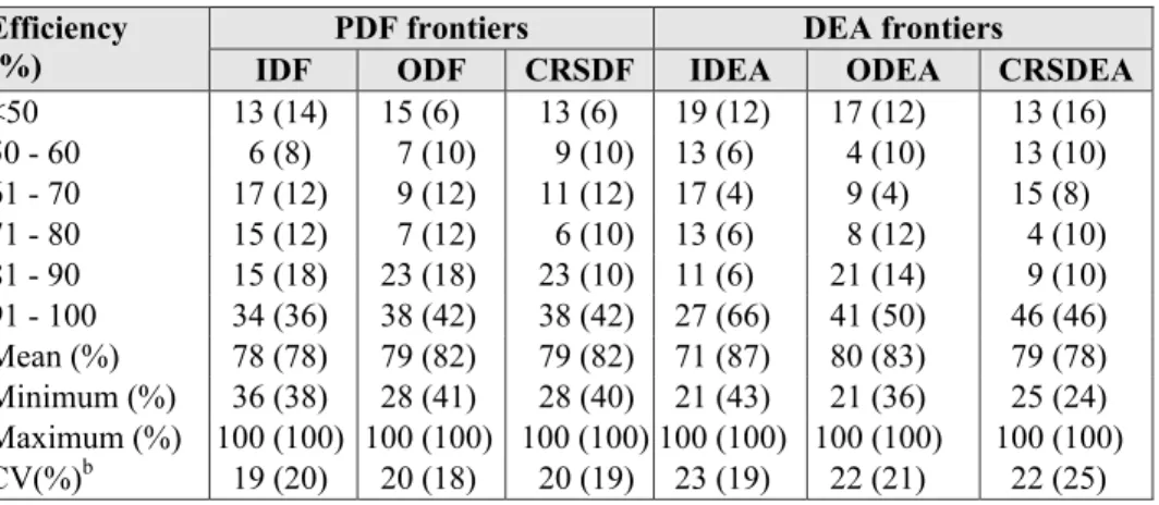
The frequency distributions and summary statistics of technical efficiency measures obtained from input distance function frontier (IDF), output distance function frontier
(ODF), CRS distance function (CRSDF), input oriented DEA frontier (IDEA), output oriented DEA frontier (ODEA), and CRS DEA frontier (CRSDEA) are presented in Table 2.
Table 2. Frequency distributions (%) and summary statistics of technical efficiency measures from PDF and DEA approaches a
PDF frontiers DEA frontiers Efficiency
(%) IDF ODF CRSDF IDEA ODEA CRSDEA
<50 13 (14) 15 (6) 13 (6) 19 (12) 17 (12) 13 (16) 50 - 60 6 (8) 7 (10) 9 (10) 13 (6) 4 (10) 13 (10) 61 - 70 17 (12) 9 (12) 11 (12) 17 (4) 9 (4) 15 (8) 71 - 80 15 (12) 7 (12) 6 (10) 13 (6) 8 (12) 4 (10) 81 - 90 15 (18) 23 (18) 23 (10) 11 (6) 21 (14) 9 (10) 91 - 100 34 (36) 38 (42) 38 (42) 27 (66) 41 (50) 46 (46) Mean (%) 78 (78) 79 (82) 79 (82) 71 (87) 80 (83) 79 (78) Minimum (%) 36 (38) 28 (41) 28 (40) 21 (43) 21 (36) 25 (24) Maximum (%) 100 (100) 100 (100) 100 (100) 100 (100) 100 (100) 100 (100) CV(%)b 19 (20) 20 (18) 20 (19) 23 (19) 22 (21) 22 (25) a
Figures in parentheses are the results excluding the three potential outliers (i.e.,n=50).
b
CV= Coefficient of variation.
The results obtained from both approaches clearly indicate that there are considerable technical inefficiencies among improved cereal technology adopters. The estimated mean technical efficiencies (TE) range from a low 71% using IDEA to a high 80% us-ing ODEA. This suggests that TE scores from DEA are highly sensitive to orientation although IDEA and ODEA results are positively and significantly correlated (ρ=0.900). On the other hand, TE estimates from PDF approaches are not as sensitive to orientation as those from DEA. The mean TE estimates from IDF and ODF are 78% and 79%, respectively, and have a positive and significant correlation (ρ=0.897). The correlations between the various sets of technical efficiency predictions are presented in Table 3.
The agreements and disagreements in the efficiency scores obtained from the two approaches are summarized in Table 4. We note that comparison of the two approaches, Table 3. Correlation table of efficiency predictions from PDF and DEA frontiers*
PDF frontiers DEA frontiers
IDF ODF CRSDF IDEA ODEA CRSDEA
IDF 1.000 0.897 0.897 0.627 0.657 0.638 ODF 1.000 1.000 0.733 0.771 0.724 CRSDF 1.000 0.732 0.771 0.723 IDEA 1.000 0.900 0.912 ODEA 1.000 0.894 CRSDEA 1.000
given an input, output, or CRS orientation is more appealing than comparison of orien-tations for a given approach as the choice of an orientation must be guided by the under-lying behavioural assumption such as cost minimization or revenue/profit maximiza-tion. An analysis of a sample without possible outliers associated with the highest and lowest TE indices is carried out to examine the relative robustness of PDF and DEA estimates. The estimates from PDF approaches are more robust than those from DEA in that they are less sensitive to outliers. The mean TE scores from IDF and ODF without the three potential outliers are 78% and 82%, respectively. The results under the CRS orientation, both with and without the outliers, are also very similar with those from IDF and ODF. The mean TE estimates from the CRSDF with and without the three out-liers are 79% and 82%, respectively. The relative robustness of the PDF approach can also be shown by comparing the proportion of technically efficient farmers with and without the three outliers (Table 2). For example, while 21% and 23% of the farmers in the original sample are technically efficient under IDF and ODF approaches, respec-tively, this has grown only to 28% in the sample without the outliers whereas it has grown from 17% to 64% under IDEA and from 34% to 48% under ODEA.
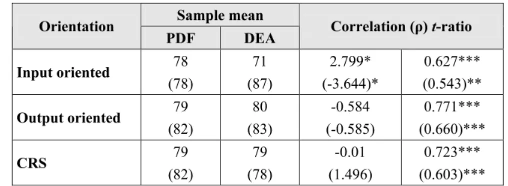
Table 4 shows that there is a significant correlation among the estimated efficiencies from the two approaches under each orientation. While TE measures from IDF are sig-nificantly higher than those from IDEA, PDF and DEA estimates are not sigsig-nificantly different under the output and CRS orientations and are highly correlated. The results compare well with those from Coelli and Perelman (1999) who also got similar PDF and DEA estimates. Although both the input and output oriented PDF could be used, the output oriented PDF results would be more appropriate given the plausibility of the as-sumption that farmers maximise their revenues given fixed factors of production such as land and family labour. Based on the preferred output oriented PDF approach, therefore, there is an average technical efficiency of 79% among improved technology adopters in eastern Ethiopia. This suggests that improved technology adopters could, on average, raise their production by 21% through improved technical efficiency alone, given their existing improved production technology.
Table 4. Mean comparison and correlations of technical efficiency rankings of the relevant orientations with and without the three outliers a
Sample mean Orientation
PDF DEA Correlation (ρ) t-ratio Input oriented 78 (78) 71 (87) 2.799* (-3.644)* 0.627*** (0.543)** Output oriented (82) 79 (83) 80 (-0.585) -0.584 (0.660)*** 0.771*** CRS 79 (82) 79 (78) -0.01 (1.496) 0.723*** (0.603)*** a
, Figures in parentheses are the results excluding the three potential outliers (i.e.,n=50).
*, Represents significance of the mean differences at the 0.01 level; ** and *** represent, re-spectively, significance of rank correlation at 0.05 and 0.01 levels.
Concluding comments
This study compares the empirical performance of parametric and non-parametric distance function methodologies with applications to improved production technology adopters in eastern Ethiopia. Technical efficiencies obtained from the two approaches are positively and significantly correlated. The results indicate substantial technical in-efficiencies of production among the sample farmers. The DEA approach is shown to be relatively more sensitive to outliers as well as orientation. Average technical efficiencies of adopters of improved technology are estimated 79% based on the preferred PDF ap-proach with the appropriate orientation, implying that the sample farmers could raise their production by an average 21% through improved technical efficiency.
The results confirm the view that food production even under improved technology in developing countries involves substantial inefficiencies due to farmers’ high unfa-miliarity with new technology coupled with poor extension, education, credit, and input supply systems. This is even more pronounced in Ethiopia where the gap between the demand for and supply of extension services is growing and consequently the services are of poor quality and have very low coverage. Further, credit and input supply con-straints are more acute thereby inhibiting proper and optimal application of new tech-nology. Therefore, policies and strategies aimed at improving the extension, credit and input supply systems will help raise the technical efficiency and productivity of farmers.
References
Aigner, D.J. & Chu, S.F. (1968) On estimating the industry production function, Ameri-can Economic Review, 58, 826-839.
Ali, M. and Byerlee, D. (1991) Economic efficiency of small farmers in a changing world: A survey of recent evidence, Journal of International Development, 3(1), 1-27.
Ali, M. and Chaudry, M.A. (1990) Inter-regional farm efficiency in Pakistan's Punjab: a frontier production function study, Journal of Agricultural Economics, 4, 162-74. Charnes, A., Cooper, W. W. and Rhodes, E. (1978). Measuring the efficiency of
deci-sion making units, European Journal of Operation Research, 2, 429-444.
Coelli, T.J. (1995) Recent developments in frontier modelling and efficiency measure-ment, Australian Journal of Agricultural Economics, 39(3 ), 219-245.
Coelli, T.J. and Perelman, S. (1996) Efficiency measurement, multiple-output technolo-gies and distance functions: With applications to European railways, CREPP working paper 96/05, University of Liege.
Coelli, T.J. & Perelman, S. (1999) A comparison of parametric and non-parametric dis-tance functions: With applications to European railways, European Journal of Operational Research, 117, 326-339.
Coelli, T.J., Prasada Rao, D.S. & Battese, G.E. (1998) An introduction to efficiency and productivity analysis. Kluwer Academic Publishers, Boston, USA.
Drake, L. and Weyman-Jones, T.G. (1996) Productive and allocative inefficiencies in UK building societies: A comparison of nonparametric and stochastic frontier techniques, The Manchester School, 64, 22-37.
Färe, R., Grosskopf, S. and Lovell, C.A.K. (1994) Production Frontiers. Cambridge University Press, Cambridge.
Färe, R., Grosskopf, S., Lovell, C.A.K. and Pasurka, C. (1989) Multilateral productivity comparisons when some outputs are undesirable: A nonparametric approach, The Review of Economics and Statistics, 71 (February), 90-98.
Färe, R., Grosskopf, S., Lovell, C. A. K. and Yaisawarng, S. (1993) Derivation of shadow prices for undesirable outputs: A distance function approach, The Review of Economics and Statistics, 75 (May), 374-80.
Ferrier, G.D. and Lovell, C.A.K. (1990) Measuring cost efficiency in banking: Econo-metric and linear programming evidence, Journal of EconoEcono-metrics, 46, 229-245. Grosskopf, S., Hayes, Taylor; K. L. and Weber; W. (1997) Budget constrained frontier
measures of fiscal equality and efficiency in schooling, The Review of Econom-ics and StatistEconom-ics, 79, 116-124.
Hailu, A. and Veeman, T.S. (2000) Environmentally sensitive productivity analysis of the Canadian pulp and paper industry, 1959-1994: An input distance function ap-proach, Journal of Environmental Economics and Management, 40, 251-274. Kalaitzandonakes, N.G. and Dunn, E.G. (1995) Technical efficiency, managerial ability
and farmer education in Guatemalan corn production: A latent variable analysis, Agricultural and Resource Economics Review, 24, 36-46.
Kalirajan, K. (1991) The importance of efficient use in the adoption of technology: A micro panel data analysis, Journal of Productivity Analysis, 2, 113-126.
Mulat, D. (1999) The challenge of increasing food production in Ethiopia, In The Ethiopian Economy: Performance and Evaluation, Proceedings of the Eighth An-nual Conference on the Ethiopian Economy (Ed.) G. Alemayehu and N. Berhanu, Nazareth, Ethiopia.
Sharma, K.R., Leung, P. and Zalleski, H.M. (1997) Productive efficiency of the swine industry in Hawaii: stochastic frontier vs data envelopment analysis, Journal of Productivity Analysis, 8, 447-459.
--- (1999) The technical, allocative, and economic efficiencies in swine production in Hawaii: A comparison of parametric and non-parametric ap-proaches, Agricultural Economics, 20, 23-35.
Shephard, R.W. (1970) Theory of Cost and Production Functions. Princeton University Press, Princeton, NJ.
Techane, A. and Mulat, D. (1999) Institutional reforms and sustainable input supply and distribution in Ethiopia, In Institutions for Rural Development, Proceedings of the 4th Annual Conference of the Agricultural Economics Society of Ethiopia(Eds.)
N. Workineh, D. Legesse, H. Abebe, and B. Solomon, Addis Ababa.
Wadud, M.A. and White, B. (2000) Farm household efficiency in Bangladesh: A com-parison of stochastic frontier and DEA methods, Applied Economics, 32, 1665-1673.
Xu, X. and Jeffrey, S.R. (1998) Efficiency and technical progress in traditional and modern agriculture: Evidence from rice production in China, Agricultural Eco-nomics, 18, 117-165.