Boise State University
ScholarWorks
Mechanical and Biomedical Engineering Faculty Publications and Presentations
Department of Mechanical and Biomedical Engineering
1-1-2013
Multi-Level Parallelism for Incompressible Flow
Computations on GPU Clusters
Dana A. Jacobsen
Boise State University
Inanc Senocak
Boise State University
NOTICE: this is the author's version of a work that was accepted for publication inParallel Computing. Changes resulting from the publishing process, such as peer review, editing, corrections, structural formatting, and other quality control mechanisms may not be reflected in this document. Changes may have been made to this work since it was submitted for publication. A definitive version was subsequently published inParallel Computing, 2012. DOI:10.1016/j.parco.2012.10.002
Multi-level Parallelism for Incompressible Flow
Computations on GPU Clusters
Dana A. Jacobsena, Inanc Senocakb,∗
a
Department of Computer Science
b
Department of Mechanical and Biomedical Engineering
c
Boise State University, Boise, ID 83725
Abstract
We investigate multi-level parallelism on GPU clusters with MPI-CUDA and hybrid MPI-OpenMP-CUDA parallel implementations, in which all computa-tions are done on the GPU using CUDA. We explore efficiency and scalability of incompressible flow computations using up to 256 GPUs on a problem with approximately 17.2 billion cells. Our work addresses some of the unique is-sues faced when merging fine-grain parallelism on the GPU using CUDA with coarse-grain parallelism that use either MPI or MPI-OpenMP for communi-cations. We present three different strategies to overlap computations with communications, and systematically assess their impact on parallel perfor-mance on two different GPU clusters. Our results for strong and weak scaling analysis of incompressible flow computations demonstrate that GPU clusters offer significant benefits for large data sets, and a dual-level MPI-CUDA im-plementation with maximum overlapping of computation and communication provides substantial benefits in performance. We also find that our tri-level MPI-OpenMP-CUDA parallel implementation does not offer a significant ad-vantage in performance over the dual-level implementation on GPU clusters with two GPUs per node, but on clusters with higher GPU counts per node or with different domain decomposition strategies a tri-level implementation may exhibit higher efficiency than a dual-level implementation and needs to be investigated further.
Keywords: GPU, hybrid MPI-OpenMP-CUDA, fluid dynamics
∗Corresponding author
Email addresses: [email protected](Dana A. Jacobsen),[email protected]
1. Introduction
1
Many applications in advanced modeling and simulation require more
2
resources than a single computing unit can provide, whether in the
prob-3
lem size or the required performance. Graphics processing units (GPUs)
4
have enjoyed rapid adoption within the high-performance computing (HPC)
5
community because GPUs enable high levels of fine-grain data parallelism.
6
The latest GPU programming interfaces such as NVIDIA’s Compute Unified
7
Device Architecture (CUDA) [1], and more recently Open Computing
Lan-8
guage (OpenCL) [2] provide the programmer a flexible model while exposing
9
enough of the hardware for optimization.
10
Current high-end GPUs can achieve high floating point throughputs by
11
combining highly parallel processing (200-800 scalar processing units per
12
GPU), high memory bandwidth and efficient thread scheduling. GPU
clus-13
ters, where fast network connected compute-nodes are augmented with latest
14
GPUs, [3] are now being used to solve challenging problems from various
do-15
mains. Examples include the 384 GPU Lincoln Tesla cluster operated by
16
the National Center for Supercomputing Applications (NCSA) at University
17
of Illinois at Urbana Champaign [4] and the 512 GPU Longhorn cluster at
18
the Texas Advanced Computing Center (TACC). Latest supercomputers too
19
allow large numbers of GPUs to be used to solve single problems. Examples
20
include the 7168 GPU Tianhe-1A [5, 6] and the 4640 GPU Dawning Nebulae
21
[7] supercomputers. These new systems are designed for high performance
22
as well as high power efficiency, which is a crucial factor in future exascale
23
computing [8].
24
2. Related Works
25
GPU computing has evolved from hardware rendering pipelines that were
26
not amenable to non-rendering tasks, to the modern General Purpose
Graph-27
ics Processing Unit (GPGPU) paradigm. Owens et al. [9] survey the early
28
history as well as the state of GPGPU computing up to 2007. The use of
29
GPUs for Euler solvers and incompressible Navier-Stokes solvers has also
30
been well documented [10–17].
31
Modern motherboards can accommodate multiple GPUs in a single
work-32
station with several TeraFLOPS of peak performance, but GPU
program-33
ming models have to be interleaved with MPI, OpenMP or Pthreads to make
use of all the GPUs in computations. In the multi-GPU computing front,
35
Thibault and Senocak [15, 16] developed a single-node multi-GPU 3D
incom-36
pressible Navier-Stokes solver with a Pthreads-CUDA implementation. The
37
GPU kernels from their study forms the internals of the present cluster
im-38
plementation. Thibault and Senocak demonstrated a speedup of 21×for two
39
Tesla C870 GPUs compared to a single core of an Intel Core 2 E8400 3.0 GHz
40
processor, 53× for two GPUs compared to an AMD Opteron 8216 2.4 GHz
41
processor, and 100× for four GPUs compared to the same AMD Opteron
42
processor. Four GPUs were able to sustain 3×speedup compared to a single
43
GPU on a large problem size. The multi-GPU implementation of Thibault
44
and Senocak does not overlap computation with GPU data exchanges.
There-45
fore, three overlapping strategies are systematically introduced and evaluated
46
in the present study.
47
Micikevicius [18] describes both single and multi GPU CUDA
implemen-48
tations of a 3D 8th-order finite difference wave equation computation. The
49
wave equation code is composed of a single kernel with one stencil
opera-50
tion, unlike CFD computations which consist of multiple inter-related kernels.
51
MPI was used for process communication in multi-GPU computing.
Micike-52
vicius uses a two stage computation where the cells to be exchanged are
com-53
puted first, then the inner cells are computed in parallel with asynchronous
54
memory copy operations and MPI exchanges. With efficient overlapping of
55
computations and copy operations, Micikevicius achieves very good scaling
56
on 4 GPUs running on two Infiniband connected nodes with two Tesla
10-57
series GPUs each, when using a large enough dataset.
58
G¨oddeke et al. [12] explored course and fine grain parallelism in a finite
59
element model for fluids or solid mechanics computations on a GPU cluster.
60
G¨oddeke et al. [19] described the application of their approach to a large-scale
61
solver toolkit. The Navier-Stokes simulations in particular exhibited limited
62
performance due to memory bandwidth and latency issues. Optimizations
63
were also found to be more complicated than simpler models such as the ones
64
they previously considered. While the small cluster speedup of a single kernel
65
is good, unfortunately acceleration of the entire model is only a modest factor
66
of two. Their model uses a nonuniform grid and multigrid solvers within a
67
finite element framework for relatively low Reynolds numbers.
68
Phillips et al. [20] describe many of the challenges that arise when
imple-69
menting scientific computations on a GPU cluster, including the host/device
70
memory traffic and overlapping execution with computation. A performance
71
visualization tool was used to verify overlapping of CPU, GPU, and
nication on an Infiniband connected 64 GPU cluster. Scalability is noticeably
73
worse for the GPU accelerated application than the CPU application as the
74
impact of the GPU acceleration is quickly dominated by the communication
75
time. However, the speedup is still notable. Phillips et al. [21] describe a
76
2D Euler Equation solver running on an 8 node cluster with 32 GPUs. The
77
decomposition is 1D, but GPU kernels are used to gather/scatter from linear
78
memory to non-contiguous memory on the device.
79
While MPI is the API typically used for network communication between
80
compute nodes, it presents a distributed memory model which can
poten-81
tially make it less efficient for processes running on the same shared-memory
82
compute node [22, 23]. For this reason, hybrid programming models
com-83
bining MPI and a threading model such as OpenMP or Pthreads have been
84
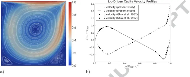
proposed with the premise that message passing overhead can be reduced,
85
increasing scalability. With two to four GPUs per compute node, a hybrid
86
MPI-OpenMP-CUDA method warrants further investigation and is studied
87
in this paper along with an MPI-CUDA method to develop a multi-level
88
parallel incompressible flow solver for GPU clusters.
89
Cappello, Olivier, and Etiemble [24–26] were among the first to present
90
the hybrid programming model of using MPI in conjunction with a
thread-91
ing model such as OpenMP. They demonstrated that it is sometimes possible
92
to increase efficiency on some codes by using a mixture of shared memory
93
and message passing models. A number of other papers followed with the
94
same conclusions [27–34]. Many of these papers also point out a number
95
of cases where the applications or computing systems are a poor fit to the
96
hybrid model, and in some cases performance decreases. Lusk and Chan
97
[35] describes using OpenMP and MPI for hybrid programming on three
98
cluster environments, including the effect the different models have on
com-99
munication with the NAS benchmarks. They claim combination of MPI and
100
OpenMP parallel programming is well fitted to modern scalable high
perfor-101
mance systems.
102
Hager, Jost, and Rabenseifner [36] give a recent perspective on the state
103
of the art techniques in hybrid MPI-OpenMP programming. Particular
at-104
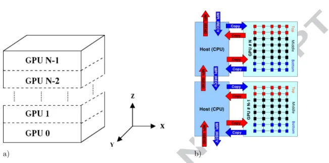
tention is given to mapping the model to domain decomposition as well as
105
overlapping methods. Results with hybrid models of the BT-MZ benchmark
106
(part of the NAS Parallel Benchmark suite) on a Cray XT5 using a hybrid
107
approach showed similar performance at 64 and fewer cores, but greatly
im-108
proved results for 128, 256, and 512 cores, where a good combination of
109
OpenMP fine-grain parallelism combined with MPI coarse-grin parallelism
can be found that matches well with the hardware. These examples also
111
take advantage of the loop scheduling features in OpenMP. Advantages in
112
fine grain parallelism like this will not be able to be taken advantage of
113
in a model where OpenMP is only used for coarse-grain data transfer and
114
synchronization.
115
Balaji et al. [37] discuss issues arising from using MPI on petascale
ma-116
chines with close to a million processors. A number of irregular MPI
collec-117
tive operations are considered to be nonscalable when applied to a very large
118
number of processes. The tested MPI implementations also allocate some
119
memory which is proportional to the number of processes, limiting
scalabil-120
ity. These as well as other limitations lead Balaji et al. to suggest a hybrid
121
threading / MPI model as one way to mitigate the issue. However, we think,
122
in the case of a typical GPU system the situation is not as bad. Because
123
the CUDA model for fine-grain parallelism manages 256 to 512 processing
124
elements within a single process, and this number will likely increase with
125
future GPUs. Hence a one million processing element GPU cluster using
126
just MPI-CUDA may have fewer than 4000 MPI processes. This suggests
127
that clusters enhanced with GPUs look well suited for petascale and
emerg-128
ing exascale architectures. Therefore, compute-intensive applications need to
129
be evaluated for parallel efficiency and performance on large GPU clusters.
130
Our study is one of few that critically evaluates multi-level parallelism of
131
incompressible flow computations on GPU clusters.
132
Nakajima [38] describes a three-level hybrid method using MPI, OpenMP,
133
and vectorization. This approach uses MPI for inter-node communication,
134
OpenMP for intra-node communication, and parallelism within the node via
135
the vector processor. It closely matches the rationale behind our hybrid
MPI-136
OpenMP-CUDA approach for a GPU cluster implementation. Nakajima’s
137
weak scaling measurements showed worse results for 64 and fewer SMP nodes,
138
but improved with 96 or more. GPU clusters with 128 or more
compute-139
nodes (256 or more GPUs) are rare at this time, but trends indicate these
140
machines will become far more common in the high performance computing
141
field [6–8].
142
While these articles show some potential benefits for using the hybrid
143
model on CPU clusters, a question is whether the same benefits will
ac-144
crue to a tri-level CUDA-OpenMP-MPI model, and whether the benefits
145
will outweigh the added software complexity. With high levels of data
par-146
allelism on the GPU, separate memory for each GPU, low device counts per
147
node, and currently small node counts, the GPU cluster model has
ous differences from dense-core CPU clusters. In this paper we investigate
149
several methods of distributing computation using a dual (MPI-CUDA) and
150
tri-level (MPI-OpenMP-CUDA) parallel programming approaches along with
151
different strategies to overlap computation and communication on GPU
clus-152
ters. We adopt MPI for coarse-grain inter-node communication, OpenMP
153
for medium-grain intra-node communication in the tri-level approach, and
154
CUDA for fine-grain parallelism within the GPUs. In all of our
implementa-155
tions, computations are entirely done on the GPU using CUDA. We use a 3D
156
incompressible flow Navier-Stokes solver to systematically assess scalability
157
and performance of multi-level parallelism on large GPU clusters.
158
3. Governing Equations and Numerical Approach
159
Navier-Stokes equations for buoyancy driven incompressible fluid flows
160
can be written as follows:
161 ∇ ·u= 0, (1) 162 ∂u ∂t +u· ∇u=− 1 ρ∇P +ν∇ 2u +f, (2)
where u is the velocity vector, P is the pressure, ρ is the density, ν is the
163
kinematic viscosity, andf is the body force. The Boussinesq approximation,
164
which applies to incompressible flows with small temperature variations, is
165
used to model the buoyancy effects in the momentum equations [39]:
166
f =g·(1−β(T −T∞)), (3)
whereg is the gravity vector, β is the thermal expansion coefficient, T is the
167
calculated temperature at the location, and T∞ is the steady state
tempera-168
ture.
169
The temperature equation can be written as [40, 41]
170
∂T
∂t +∇ ·(uT) =α∇ 2
T + Φ, (4)
where α is the thermal diffusivity and Φ is the heat source.
171
The buoyancy-driven incompressible form of the Navier-Stokes equations
172
(Eqs. 1–4) do not have an explicit equation for pressure. Therefore, we use
173
the projection algorithm of Chorin [42], where the velocity field is first
pre-174
dicted using the momentum equations without the pressure gradient term.
a) b)
Figure 1. Lid-driven cavity simulation with Re = 1000 on a 256 ×32×
256 grid. 3D computations were used and a 2D center slice is shown. a) Velocity streamlines and velocity magnitude distribution. b) Comparison to the benchmark data from Ghia et al. [44].
The resulting predicted velocity field does not satisfy the divergence free
con-176
dition. The divergence free condition is then enforced on the velocity field
177
at time t+ 1, to derive a pressure Poisson equation from the momentum
178
equations given in Eq. (2). We solve the discretized versions of the resulting
179
equations on a uniform Cartesian staggered grid with second order central
180
difference scheme for spatial derivatives and a second order accurate
Adams-181
Bashforth scheme for time derivatives. The pressure Poisson equation can
182
be solved using either a fixed iteration Jacobi solver or a parallel geometric
183
multigrid solver [43]. Both solvers are available in our code. We do not
184
activate the geometric multigrid solver in certain computations where we
in-185
vestigate dual- and tri-level parallelism, because the amalgamated parallel
186
implementation of the multigrid method complicates the detailed analysis of
187
scaling and breakdown of communication timings due to the inherent
algo-188
rithmic complexity in the method.
189
Validation on a number of test cases including the well-known lid-driven
190
cavity and natural convection in heated cavity problems [44, 45] were used
191
to compare the overall solutions to known results. Figure 1 presents the
192
results of a lid-driven cavity simulation with a Reynolds number 1000 on a
193
256 ×32×256 grid. Figure 1a shows the velocity magnitude distribution
a) b)
Figure 2. Natural convection in a cavity using a 128×16×128 grid and Prandtl number 7, with a 2D center slice shown. a) Streamlines for Rayleigh number 200,000. b) Isotherms and temperature distribution for Rayleigh number 200,000.
and streamlines at mid-plane. As expected, the computations capture the
195
two corner vortices at steady-state. In Fig. (1b), the horizontal and vertical
196
components of the velocity along the centerlines ar e compared to the
bench-197
mark data of Ghia et al. [44]. The results agree well with the benchmark
198
data. The numerical results for the tri-level and dual-level parallel versions
199
do not differ.
200
We simulate the natural convection in a heated cavity problem to test our
201
buoyancy-driven incompressible flow computations on a 128×16×128 grid.
202
Figure 2 presents the natural convection patterns and isotherms for Rayleigh
203
(Ra) numbers of 200,000 and a Prandtl (Pr) number of 7.0. Lateral walls
204
have constant temperature boundary conditions with one of the walls having
205
a higher temperature than the wall on the opposite side. Top and bottom
206
walls are insulated. Fluid inside the cavity is heated on the hot lateral wall
207
and rises due to buoyancy effects, whereas on the cold wall it cools down
208
and sinks, creating a circular convection pattern inside the cavity. Although
209
not shown in the present paper, our results agree well with similar results
210
presented in Griebel et al. [40]. A direct comparison is available in Jacobsen
211
[17]. Figure 3 presents a comparison of the horizontal centerline temperatures
212
for a heated cavity with Ra=100,000 and Pr=7.0 along with reference data
Figure 3. Centerline temperature for natural convection in a cavity with Prandtl number 7 and Rayleigh number 100,000, using a 256×16×256 grid with a 2D center slice used. Comparison is shown to data from Wan et al. [45].
from Wan et al. [45]. Our results are in very good agreement.
214
Aside from these benchmark cases, our CFD solver can compute flow
215
around embedded obstacles such as urban areas and complex terrain can be
216
found in [17, 46, 47]
217
4. Multi-level Parallelism
218
Multiple programming APIs along with a domain decomposition
strat-219
egy for data-parallelism is required to achieve high throughput and scalable
220
results from a CFD model on a multi-GPU platform. For problems that
221
are small enough to run on a single GPU, overhead time is minimized as
222
no GPU/host communication is performed during the computation, and all
223
optimizations are done within the GPU code. When more than one GPU
224
is used, cells at the edges of each GPU’s computational space must be
com-225
municated to the GPUs that share the domain boundary so they have the
226
current data necessary for their computations. Data transfers across the
227
neighboring GPUs inject additional latency into the implementation which
228
can restrict scalability if not properly handled. For these reasons we
investi-229
gate multi-level parallelism on GPU clusters with different implementations
a) b)
Figure 4. The domain decomposition. a) The decomposition of the full computational domain to the individual GPUs. b) An overview of the com-munication, GPU memory transfers, and the intra-GPU 1D decomposition used for overlapping.
to improve the performance and scalability of our Navier-Stokes solver.
231
4.1. Domain Decomposition 232
A 3D Cartesian volume is decomposed into 1D slices. These slices are
233
then partitioned among the GPUs on the cluster to form a 1D domain
de-234
composition. The 1D decomposition is shown in Figure 4a. After each GPU
235
completes its computation, the edge cells (“ghost cells”) must be exchanged
236
with neighboring GPUs. Efficiently performing this exchange process is
cru-237
cial to cluster scalability as we demonstrate in section 5.
238
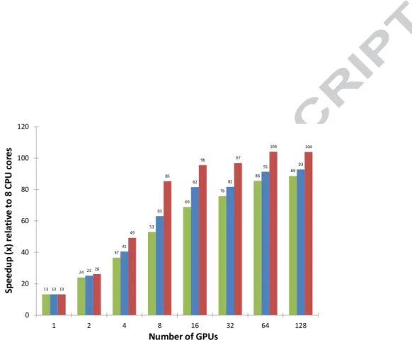
While a 1D decomposition leads to more data being transferred as the
239
number of GPUs increases, there are advantages to the method when
us-240
ing CUDA. In parallel CPU implementations, host memory access can be
241
performed on non-contiguous segments with a relatively small performance
242
loss. The MPI CART routines supplied by MPI allow efficient management of
243
virtual topologies, making the use of 2D and 3D decompositions easy and
244
efficient. In contrast, the CUDA API only provides a way to transfer linear
245
segments of memory between the host and the GPU. Hence, 2D or 3D
de-246
compositions for GPU implementations must either use nonstandard device
memory layouts which may result in poor GPU performance, or run separate
248
kernels to perform gather/scatter operations into a linear buffer suitable for
249
the cudaMemcpy() routine. These routines add significant time and hinder
250
overlapping methods. For these reasons, the 1D decomposition was deemed
251
best for moderate size clusters such as the ones used in this study.
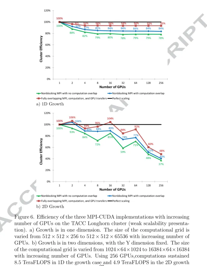
252
To accommodate overlapping, a further 1D decomposition is applied
253
within each GPU. Figure 4b indicates how the 1D slices within each GPU
254
are split into a top, bottom, and middle section. When overlapping
commu-255
nication and computation, the GPU executes each separately such that the
256
memory transfers and MPI communication can happen simultaneously with
257
the computation of the middle portion.
258
4.2. Dual-Level MPI-CUDA Implementations 259
The work by Thibault and Senocak [15, 16] showed how an incompressible
260
Navier-Stokes solver written for a single GPU can be extended to multiple
261
GPUs by interleaving CUDA with Pthreads. The full 3D domain is
decom-262
posed across threads in one dimension, splitting on the Z axis. The resulting
263
partitions are then solved using one GPU per thread. No effort was made
264
to hide latencies arising from GPU data transfers or Pthreads
synchroniza-265
tion. To solve the restrictions of the shared memory model of Thibault and
266
Senocak, we adopt MPI as the mechanism for communication between GPUs,
267
and introduce three strategies to overlap computations on the GPU with data
268
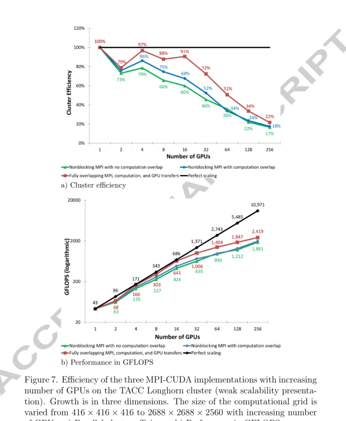
copying to and from the GPU and MPI communication across the network.
269
In our present implementation, a single MPI process is started per GPU,
270
and each process is responsible for managing its GPU and exchanging data
271
with its neighbor processes. Since we must ensure that each process is
as-272
signed a unique GPU identifier, an initial mapping of hosts to GPUs is
per-273
formed. A master process gathers all the host names, assigns GPU identifiers
274
to each host such that no process on the same host has the same identifier,
275
and scatters the result back. At this point thecudaSetDevice()call is made
276
on each process to map one of the GPUs to the process which assures that
277
no other process on the same node will map to the same GPU. All ghost cell
278
exchanges are done via MPI Isend and MPI Irecv. Overlap of computations
279
with inter-node and intra-node data exchanges is accomplished to better
uti-280
lize the cluster resources. All three of the implementations have much in
281
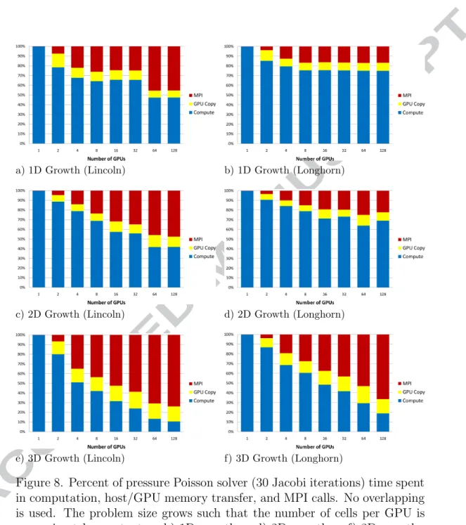
common, with differences in the way data exchanges are implemented. It is
282
shown in section 5 that implementation details in the data exchanges have a
283
large impact on performance.
for (t=0; t < time_steps; t++) {
adjust_timestep();
for (stage = 0; stage < num_timestep_stages; stage++) { temperature <<<grid,block>>> (u,v,w,phiold,phi,phinew); ROTATE_POINTERS(phi,phinew);
temperature_bc <<<grid,block>>> (phi); EXCHANGE(phi);
turbulence <<<grid,block>>> (u,v,w,nu); turbulence_bc <<<grid,block>>> (nu); EXCHANGE(nu);
momentum <<<grid,block>>> (phi,uold,u,unew,vold,v,vnew,wold,w,wnew); momentum_bc <<<grid,block>>> (unew,vnew,wnew);
EXCHANGE(unew,vnew,wnew); }
divergence <<<grid,block>>>(unew,vnew,wnew,div); // Iterative or multigrid solution
pressure_solve(div,p,pnew);
correction <<<grid,block>>> (unew,vnew,wnew,p); momentum_bc <<<grid,block>>> (unew,vnew,wnew); EXCHANGE(unew,vnew,wnew);
ROTATE_POINTERS(u,unew); ROTATE_POINTERS(v,vnew); ROTATE_POINTERS(w,wnew); }
Listing 1. Host code for the projection algorithm to solve buoyancy driven incompressible flow equations on multi-GPU platforms. The EXCHANGE step updates the ghost cells for each GPU with the contents of the data from the neighboring GPU.
// PART 1: Interleave non-blocking MPI calls with device // to host memory transfers of the edge layers. // Communication to south
MPI_Irecv(new ghost layer from north)
cudaMemcpy(south edge layer from device to host) MPI_Isend(south edge layer to south)
// Communication to north
MPI_Irecv(new ghost layer from south)
cudaMemcpy(north edge layer from device to host) MPI_Isend(north edge layer to north)
// ... other exchanges may be started here, before finishing in order // PART 2: Once MPI indicates the ghost layers have been received, // perform the host to device memory transfers.
MPI_Wait(new ghost layer from north)
cudaMemcpy(new north ghost layer from host to device) MPI_Wait(new ghost layer from south)
cudaMemcpy(new south ghost layer from host to device)
MPI_Waitall(south and north sends, allowing buffers to be reused) Listing 2. An EXCHANGE operation overlaps GPU memory copy operations with asynchronous MPI calls for communication.
The projection algorithm is composed of distinct steps in the solution
285
of the fluid flow equations. Listing 1 shows an outline of the basic
imple-286
mentation using CUDA kernels to perform each step. The steps marked as
287
EXCHANGE are where ghost cells for each GPU are filled in with the calculated
288
contents of their neighboring GPUs. The most basic exchange method is to
289
call cudaMemcpy() to copy the edge data to host memory, MPI exchange
us-290
ing MPI Send and MPI Recv, and finally cudaMemcpy() to copy the received
291
edge data to device memory. This is straightforward, but all calls are
block-292
ing which greatly hinders performance. Therefore, we have not pursued this
293
basic implementation in the present study.
294
4.2.1. Non-blocking MPI with No Overlapping of Computation 295
The first implementation uses non-blocking MPI calls [50] to offer a
sub-296
stantial benefit over the blocking approach, which we do not pursue. Our
297
first implementation does not overlap computation although it tries to
lap memory copy operations. The basic EXCHANGE operation is shown in
299
Listing 2. In this approach, none of the device/host memory operations nor
300
any MPI communication happens until the computation of the entire domain
301
has completed. The MPI communication is able to overlap with the CUDA
302
memory operations. When multiple arrays need to be exchanged, such as the
303
three momentum components, the components may be interleaved such that
304
the MPI send and receive for one edge of the first component is in progress
305
while the memory copy operations for the later component are proceeding.
306
This is done by starting part 1 for each component in succession, then part
307
2 for each component.
308
4.2.2. Overlapping Computation with MPI Communications 309
The second implementation for exchanges aims to overlap the CUDA
310
computation with the CUDA memory copy operations and the MPI
com-311
munication. We split the CUDA kernels into three calls such that the edges
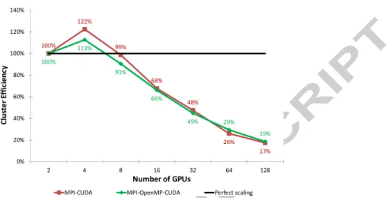
312
can be done separately from the middle. This has a very large impact on
313
the cluster performance as long as the domain is large enough to give each
314
GPU enough work to do. The body of the pressure kernel loop when using
315
this method is shown in Listing 3. Rather than perform the computation
316
on the entire domain before starting the exchange, the kernel is started with
317
just the edges being computed. The first portion of the previously shown
318
non-blocking MPI EXCHANGE operation is then started, which does device
319
to host memory copy operations followed by non-blocking MPI
communica-320
tions. The computation on the middle portion of the domain can start as
321
soon as the edge layers have finished transferring to the host, and operates
322
in parallel with the MPI communication. The last part of the non-blocking
323
MPI EXCHANGE operation is also identical and is run immediately after the
324
middle computation is started. While this implementation results in
signifi-325
cant overlap, it is possible to improve on it by overlapping the computation
326
of the middle portion with the memory transfer of the edge layers as shown
327
in the final implementation.
328
4.2.3. Overlapping Computation with MPI Communications and GPU Trans-329
fers 330
The final implementation is enabled by CUDA streams, and uses
asyn-331
chronous methods to start the computation of the middle portion as soon
332
as possible, thereby overlapping computation, memory operations, and MPI
333
communication. A similar approach is described in Micikevicius [18]. This
// The GPU domain is decomposed into three sections: // (1) top edge, (2) bottom edge, and (3) middle // Which of them the kernel should process is indicated // by a flag given as an argument.
pressure <<<grid_edge,block>>> (edge_flags, div,p,pnew); // The cudaMemcpy calls below will not start until // the previous kernels have completed.
// This is identical to part 1 of the EXCHANGE operation. // Communication to south
MPI_Irecv(new ghost layer from north)
cudaMemcpy(south edge layer from device to host) MPI_Isend(south edge layer to south)
// Communication to north
MPI_Irecv(new ghost layer from south)
cudaMemcpy(north edge layer from device to host) MPI_Isend(north edge layer to north);
pressure <<<grid_middle,block>>> (middle_flag, div,p,pnew); // This is identical to part 2 of the EXCHANGE operation. MPI_Wait(new ghost layer from north)
cudaMemcpy(new north ghost layer from host to device) MPI_Wait(new ghost layer from south)
cudaMemcpy(new south ghost layer from host to device)
MPI_Waitall(south and north sends, allowing buffers to be reused) pressure_bc <<<grid,block>>> (pnew);
ROTATE_POINTERS(p,pnew);
Listing 3. An example Jacobi pressure loop, showing how the CUDA kernel is split to overlap computation with MPI communication.
pressure <<<grid_edge,block, stream[0]>>> (edge_flags, div,p,pnew); // Ensure the edges have finished before starting the copy
cudaThreadSynchronize();
cudaMemcpyAsync(south edge layer from device to host, stream[0]) cudaMemcpyAsync(north edge layer from device to host, stream[1]) pressure <<<grid_middle,block, stream[2]>>> (middle_flag, div,p,pnew); MPI_Irecv(new ghost layer from north)
cudaStreamSynchronize(stream[0]); MPI_Isend(south edge layer to south) MPI_Irecv(new ghost layer from south) cudaStreamSynchronize(stream[1]); MPI_Isend(north edge layer to north); MPI_Wait(south receive to complete)
cudaMemcpyAsync(new south ghost layer from host to device, stream[0]) MPI_Wait(north receive to complete)
cudaMemcpyAsync(new north ghost layer from host to device, stream[1]) // Ensure all streams are done, including copy operations and computation cudaThreadSynchronize();
pressure_bc <<<grid,block>>> (pnew); ROTATE_POINTERS(p,pnew);
Listing 4. CUDA streams are used to fully overlap computation, memory copy operations, and MPI communication in the pressure loop.
method has the highest amount over overlapping, and is expected to have
335
the best performance at large scales. The body of the pressure kernel loop
336
when using this method is shown in Listing 4.
337
It is important to note that the computations inside the CUDA kernels
338
need minimal change, and the same kernel can be used for all three
imple-339
mentations. A flag is sent to each kernel to indicate which portions (top,
340
bottom, middle) it is to compute, along with an adjustment of the CUDA
341
grid size so the proper number of GPU threads are created. Since GPU
342
kernels tend to be highly optimized, minimizing additional changes in kernel
343
code is desirable.
344
4.3. Tri-Level MPI-OpenMP-CUDA Implementation 345
GPU cluster nodes are becoming denser with multiple GPUs per node
346
[51]. Therefore we add a threading model to investigate whether additional
347
efficiency can be gained from removing redundant message passing when
348
processes are on the same host and communication and synchronization are
349
handled by a hybrid MPI-OpenMP model. The effectiveness of this solution
350
depends on a number of factors, with some barriers to effectiveness being:
351
• Density of nodes. With more GPUs per node, the potential
effective-352
ness can be increased. Only clusters with two GPUs per node were
353
available for the present study.
354
• MPI implementation efficiency. The OpenMPI 1.3.2 software on the
355
NCSA Lincoln Tesla cluster seems reasonably well optimized. Goglin
356
[52] discusses optimizations of MPI implementations to improve
intra-357
node efficiency. A number of optimizations have been performed on
358
MPI implementations since the early hybrid model papers were
writ-359
ten, including a reduction in the number of copies involved. Since the
360
application being studied only uses OpenMP and MPI for coarse-grain
361
parallelism, any benefits in latency for small transactions will not have
362
an impact.
363
• A large number of nodes. Many of the hybrid model papers note
ben-364
efits occurring only as the number of nodes grows [26, 36, 38]. While
365
the 64-node 128-GPU implementation used in this study is larger than
366
many published cluster results, it may still be too small to see an
ap-367
preciable benefit.
• A good match between the hardware, the threading models, and the
do-369
main decomposition. A number of hybrid model papers show
applica-370
tion / hardware combinations that show reduced performance with the
371
hybrid model [26, 28, 30, 35].
372
• Interactions between OpenMPI, OpenMP, and CUDA can exist. For
373
instance, the default OpenMPI software on the NCSA Lincoln Tesla
374
cluster is compiled without threading support.
375
There are two popular threading models in use today: POSIX Threads
376
(Pthreads) and OpenMP. We consider OpenMP, because it has become the
377
dominant method for shared memory parallelism in the HPC community. In
378
our implementation the thread level parallelism is on a coarse grain level,
379
since CUDA is handling the fine grain parallelism. We do not consider a
380
more general approach where OpenMP can be used to perform some of the
381
computations on multi-core CPUs in addition to computations on the GPU.
382
MPI defines four levels of thread safety: SINGLE, where only one thread
383
is allowed. FUNNELED is the next level, where only a single master thread
384
on each process may make MPI calls. The third level, SERIALIZED, allows
385
any thread to make MPI calls, but only one at a time is using MPI. Finally,
386
MULTIPLE allows complete multithreaded operation, where multiple threads
387
can simultaneously call MPI functions.
388
With many clusters having pre-installed versions of MPI libraries,
some-389
times with custom network infrastructure, it is not always possible to have
390
access to the highest (MULTIPLE) threading level. Additionally, this level
391
of threading support typically comes with some performance loss, so lower
392
levels are preferred if they do not otherwise hinder parallelism [53]. Three
393
implementations were created, using theSERIALIZED,FUNNELED, andSINGLE 394
levels. The first implementation used one thread per GPU, with each thread
395
responsible for any possible MPI communications with neighboring nodes.
396
The second used N+ 1 threads for N GPUs, where a single thread per node
397
handles all MPI communications and the other threads manage the GPU
398
work. This can help alleviate resource contention between MPI and GPU
399
copies, since each activity is on its own thread. Additionally this lets one use
400
theFUNNELEDlevel, which increases portability and possibly can increase
per-401
formance. Lastly, the third version uses OpenMP directives to only perform
402
MPI calls inside single-threaded sections.
403
Similar to the dual-level MPI-CUDA testing, simulation runs were
per-404
formed on the NCSA Lincoln Tesla cluster for the tri-level parallel
// COMPUTE EDGES if (threadid > 0)
pressure <<<grid_edge,block>>> (edge_flags, div,p,pnew); #pragma omp single
{
MPI_Irecv(new ghost layer from north) }
if (threadid > 0)
cudaMemcpy(south edge layer from device to host) // Ensure all threads have completed copies #pragma omp barrier
#pragma omp single {
MPI_Isend(south edge layer to south) MPI_Irecv(new ghost layer from south) }
if (threadid > 0)
cudaMemcpy(north edge layer from device to host) // Ensure all threads have completed copies #pragma omp barrier
#pragma omp single {
MPI_Isend(north edge layer to north) }
// COMPUTE MIDDLE if (threadid > 0)
pressure <<<grid_middle,block>>> (middle_flag, div,p,pnew); #pragma omp single
{
MPI_Wait(new ghost layer from north) MPI_Wait(new ghost layer from south) }
// Ensure all threads wait for MPI communication #pragma omp barrier
if (threadid > 0) {
cudaMemcpy(new north ghost layer from host to device) cudaMemcpy(new south ghost layer from host to device) }
// Ensure all threads have completed copies #pragma omp barrier
#pragma omp single {
MPI_Waitall(south and north sends, allowing buffers to be reused) }
if (threadid > 0)
pressure_bc <<<grid,block>>> (pnew); ROTATE_POINTERS(p,pnew);
Listing 5. An example Jacobi pressure loop using tri-level MPI-OpenMP-CUDA and simple computational overlapping. This uses the SINGLE thread-ing level.
tation. At the time this study was performed, the MPICH2 implementation
406
on NCSA Lincoln had interactions with the CUDA pinned memory support,
407
making it very slow for the CUDA Streams overlapping cases. OpenMPI was
408
used instead. But, unfortunately, the OpenMPI versions available on NCSA
409
Lincoln do not support any threading level other than SINGLE, and optimal
410
network performance was not obtainable with custom compiled versions by
411
the first author. Hence only the last implementation was used. An example
412
implementation is shown in Listing 5, where simple computational
overlap-413
ping is performed. CUDA computations are performed on threads 1−N,
414
while MPI calls are performed on the single thread 0. With a FUNNELED
hy-415
brid implementation, the omp master pragma would be used instead, with
416
care taken since it has no implied barrier as omp single does.
417
4.4. Parallel Geometric Multigrid Method 418
Solution of complex incompressible flows benefits substantially from an
419
advanced solver for the pressure Poisson equation, such as a multigrid (MG)
420
method. The parallel geometric multigrid method that we implement in this
421
study is built upon the strategies and lessons learned in previous sections.
422
Based on the performance results obtained from parallel computations that
423
adopt the Jacobi solver, we choose to follow the MPI-CUDA
implementa-424
tion described in section 4.2.3 in our MG method implementation. The 3D
425
geometric MG method is composed of therestriction, smoothing,and prolon-426
gation steps. In the restriction step we use a 27-point full weighting scheme
427
to restrict the residual solution from the fine grid to the next coarse grid
428
level. The prolongation operator is the inverse operator of the restriction
429
step. Therefore, we use a trilinear interpolation in the prolongation stage.
430
In the smoothing stage, we use a weighted (ω = 0.86) Jacobi solver with 3
431
to 4 iterations as the smoother for 3D computations.
432
Different schemes can be adopted to coarsen the grid in the MG method
433
[56]. In our implementation, we use the V-cycle, which is adequate for the
434
solution of pressure Poisson equation resulting from incompressible flow
for-435
mulations. We develop an amalgamation strategy to overcome the
data-436
starvation issue that arises in a multi-GPU implementation of the MG method.
437
Basically, when the mesh at the finest level is divided and distributed over
438
the GPUs, data-starvation per GPU is inevitable because of the inherent
439
grid coarsening strategy in the MG method. When the coarsest grid per
440
GPU is reached, the overall solution has not reached the deepest level in the
441
V-cycle. We call the implementation that halts the grid coarsening process
when the coarsest mesh per GPU is reached as the truncated MG method.
443
Depending on the size of the mesh and the number of GPUs deployed in the
444
computations, truncating the MG cycle can substantially degrade the
supe-445
rior convergence rate of the MG method. To avoid this issue, we develop
446
an amalgamation strategy to complete the V-cycle to its full-depth for the
447
whole mesh. Our amalgamation strategy make use of the collective
commu-448
nication in the MPI library. Specifically, we use the MPI Gather function to
449
reconstruct the mesh on a single GPU, and continue with the V-cycle down
450
to its full-depth until the coarsest mesh for the overall domain is reached.
451
Once the coarse grid solution is performed on a single GPU, we proceed
452
with the V-cycle on a single GPU and scatter the information to all GPUs
453
with an MPI Scatter function at the same MG level where the
amalgama-454
tion to a single GPU took place. The amalgamation strategy enables us to
455
achieve the superior efficiency of the MG method in a parallel multi-GPU
456
implementation.
457
5. Performance Results from NCSA Lincoln and TACC Longhorn
458
Clusters
459
The NCSA Lincoln cluster consists of 192 Dell PowerEdge 1950 III servers
460
connected via InfiniBand SDR (single data rate) [54]. Each compute node
461
has two quad-core 2.33 GHz Intel E5410 processors and 16GB of host
mem-462
ory. The cluster has 96 NVIDIA Tesla S1070 accelerator units each housing
463
four C1060-equivalent Tesla GPUs. An accelerator unit is shared by two
464
servers via PCI-Express ×8 connections. Hence, a compute-node has access
465
to two GPUs. For the present study, performance measurements for 64 of the
466
192 available compute-nodes in the NCSA Lincoln Tesla cluster are shown,
467
with up to 128 GPUs being utilized. The CUDA 3.0 Toolkit was used for
468
compilation and runtime, gcc 4.2.4 was the compiler used, and OpenMPI
469
1.3.2 was used for the MPI library.
470
The TACC Longhorn cluster consists of 240 Dell R610 compute nodes
471
connected via InfiniBand QDR (quad data rate). Each compute node has
472
two quad-core 2.53 GHz Intel E5540 Nehalem processors and 48GB of host
473
memory. The cluster has 128 NVIDIA QuadroPlex S4 accelerator units each
474
housing four FX5800 GPUs. An accelerator unit is shared by two servers via
475
PCI-Express 2.0×16 connections. Performance of the GPU units is similar to
476
the Lincoln cluster, however the device/host memory bandwidth is more than
477
2× higher and the cluster interconnect is 4× faster. For the present study,
Figure 5. Speedup on the NCSA Lincoln Tesla cluster from the three MPI-CUDA implementations relative to the Pthreads parallel CPU code using all 8 cores on a compute-node. The lid-driven cavity problem is solved on a 1024×64×1024 grid with fixed number of iterations and time steps.
performance measurements for 128 of the 240 available compute-nodes in the
479
TACC Longhorn cluster are shown, with up to 256 GPUs being utilized. The
480
CUDA 3.0 Toolkit was used for compilation and runtime, gcc 4.1.2 was the
481
compiler used, and OpenMPI 1.3.3 was used for the MPI library.
482
Single GPU performance has been studied relative to a single CPU
proces-483
sor in many studies. Such performance comparisons are adequate for desktop
484
GPU platforms. On a multi-GPU cluster, a fair comparison should be based
485
on all the available CPU resources in the cluster. To partially address this
486
issue, the CPU version of the CFD code is parallelized with Pthreads to use
487
the eight CPU cores available on a single compute-node of the NCSA
Lin-488
coln cluster [15, 16]. Identical numerical methods are used in the CPU and
489
GPU code for the tests performed. In Thibault and Senocak [16], the
per-490
formance of the CPU version of the code was investigated and the GFLOPS
491
performance was found to be comparable to the NPB benchmark codes.
492
A lid-driven cavity problem at a Reynolds number of 1000 was chosen for
493
performance measurements. Measurements were performed for both strong 494
scaling where the problem size remains fixed as the number of processing
495
elements increases, and weak scaling where the problem size grows in direct
496
proportion to the number of processing elements. Measurements for the CPU
497
application were done using the Pthreads shared-memory parallel
implemen-498
tation using all eight CPU cores on a single compute-node of the NCSA
499
Lincoln cluster. All measurements include the complete time to run the
ap-500
plication including setup and initialization, but do not include I/O time for
501
writing out the results. Single precision was used in all computations.
502
Strong Scaling Analysis 503
Figure 5 shows the speedup of the MPI-CUDA implementation of our
504
flow solver relative to the performance of the CPU version of our solver
505
using Pthreads. The computational performance on a single compute-node
506
with 2 GPUs was 26×faster than 8 Intel Xeon cores, and 64 compute-nodes
507
with 128 GPUs performed up to 104× faster than 8 Intel Xeon cores. In
508
all configurations the fully overlapped implementation performed faster than
509
the first implementation that did not perform overlapping. Additionally, the
510
final fully overlapping implementation performs fastest in all configurations
511
with more than one GPU, and shows a significant benefit with more than four
512
GPUs. With the fixed problem size, the amount of work to do on each node
513
quickly drops — on a single GPU a single pressure iteration takes under
514
10ms of compute time. Little gain is seen beyond 16 GPUs on this fixed
size problem, which highlights the fact that GPU clusters are well-suited for
516
problems with large data sets.
517
Weak Scaling Analysis 518
All three MPI-CUDA implementations presented in section 4.2 were also
519
run with increasing problem sizes such that the memory used per GPU was
520
approximately equal. The analysis is commonly referred to as weak scalabil-521
ity. Simulations such as channel or duct flows can lead to extension of the
522
whole domain in one of the three dimensions as the problem size increases. In
523
this case the height and depth of a channel is fixed, while the width increases
524
relative to the number of GPUs. For the 1D network decomposition
per-525
formed in our flow solver, the amount of data transferred between each GPU
526
will be constant, as will the domain dimensions on each GPU. Therefore we
527
expect the scalability to be excellent.
528
Figure 6a indicates how scalability with the fully overlapped
implementa-529
tion performs so well in this one dimensional scaling case, dropping from 94%
530
with 4 GPUs to only 93% with 128 GPUs. Note that four GPUs is the first
531
case where the network is utilized. The results from the TACC Longhorn
532
cluster shows a consistent behavior, with only a 1% drop in efficiency from
533
4 GPUs to 256 GPUs. The fully overlapped MPI-CUDA implementation
534
shows a definite advantage over the other two MPI-CUDA implementations.
535
Figure 6b shows the parallel efficiency when the computational domain
536
grows in two dimensions during a weak scaling analysis. This is a very
com-537
mon scenario seen in such examples as many lid-driven cavity and
buoyancy-538
driven cases, as well as flow in complex terrain, where covering a larger
phys-539
ical area (e.g. more square blocks in an urban simulation) involves growth
540
in the horizontal dimensions, while the number of cells used for height
re-541
mains constant. On the TACC Longhorn cluster, 256 GPUs were utilized
542
on 128 compute-nodes to sustain an 4.9 TeraFLOPS performance. With
ap-543
proximately 400GB of memory used during the computation on 128 GPUs,
544
it is not possible to directly compare this to a single node CPU
implemen-545
tation on traditional machines. Figure 6b also shows the clear advantage
546
of overlapping computation and communication. Parallel efficiency in the
547
two-dimensional growth problem with full overlapping is excellent through
548
64 GPUs, and parallel efficiency drops to 60% beyond 64 GPUs.
549
One obvious feature of Figure 6(b) is that efficiency does not fall in
550
a smooth fashion with increasing GPUs, but steps up and down with an
a) 1D Growth
b) 2D Growth
Figure 6. Efficiency of the three MPI-CUDA implementations with increasing number of GPUs on the TACC Longhorn cluster (weak scalability presenta-tion). a) Growth is in one dimension. The size of the computational grid is varied from 512×512×256 to 512×512×65536 with increasing number of GPUs. b) Growth is in two dimensions, with the Y dimension fixed. The size of the computational grid is varied from 1024×64×1024 to 16384×64×16384 with increasing number of GPUs. Using 256 GPUs,computations sustained 8.5 TeraFLOPS in 1D the growth case and 4.9 TeraFLOPS in the 2D growth
overall decreasing trend. This is related to an interaction between the
two-552
dimensional problem size growth and the structure of the CUDA kernels.
553
The mechanism of having each thread loop over all the Z planes is very
effi-554
cient, however the CUDA kernel throughput strongly changes as the numbers
555
of threads (the X and Y dimensions) relative to the number of Z planes per
556
GPU is varied. Earlier implementations of the kernels, as seen in Jacobsen
557
et al. [55], show much less variability, but overall performance is lower — for
558
a similar problem the single GPU performance is 33 GFLOPS vs. 41 for the
559
current code, and 2.4 TFLOPS vs. 2.9 TFLOPS with 128 GPUs.
560
Figure 7 presents the weak scaling analysis for a growth in three
dimen-561
sions of the computational domain on the Longhorn cluster. Figure 7(a)
562
indicates how scalability with the fully overlapped implementation trails off
563
sharply at 16 GPUs, and the gap between the overlapping implementations
564
and non-overlapping narrows. The reasons for this behavior are examined
565
in the next section. Figure 7(b) shows the sustained GFLOPS performance
566
on a logarithmic scale. With 256 GPUs, 2.4 TeraFLOPS was sustained with
567
the fully overlapped implementation. Note that for the 1D growth case, 9.5
568
TeraFLOPS was sustained using the same number of GPUs.
569
Further Remarks on Scalability 570
NCSA Lincoln cluster was transformed into a GPU cluster from an
ex-571
isting CPU cluster. The connection between the compute-nodes and the
572
Tesla GPUs are through PCI-Express Gen 2 ×8 connections rather than
573
×16. Measured bandwidth for pinned memory is approximately 1.6 GB/s,
574
which is significantly slower than the 5.6 GB/s measured on a local
worksta-575
tion with PCIe Gen 2 ×16 connections to Tesla C1060s. Kindratenko et al.
576
[54] observed a low host-device bandwidth on Lincoln cluster, and suggested
577
further investigations. This observed low-bandwidth issue with the Lincoln
578
cluster has an impact on our results.
579
We performed bandwidth measurements on the TACC Longhorn
clus-580
ter which uses GPUs with similar performance (Quadroplex 2200 S4 on
581
Longhorn, Tesla S1070 on Lincoln). However, measured device/host memory
582
transfers are over 2× faster on Longhorn, and its Infiniband QDR shows a
583
4× increase in interconnect bandwidth with simple benchmarks. It should
584
also be pointed out that as the CUDA kernels are optimized and run faster,
585
less time becomes available for overlapping communications, leading to a loss
586
in parallel efficiency.
a) Cluster efficiency
b) Performance in GFLOPS
Figure 7. Efficiency of the three MPI-CUDA implementations with increasing number of GPUs on the TACC Longhorn cluster (weak scalability presenta-tion). Growth is in three dimensions. The size of the computational grid is varied from 416×416×416 to 2688×2688×2560 with increasing number of GPUs. a) Parallel cluster efficiency, b) Perfomance in GFLOPS.
a) 1D Growth (Lincoln) b) 1D Growth (Longhorn)
c) 2D Growth (Lincoln) d) 2D Growth (Longhorn)
e) 3D Growth (Lincoln) f) 3D Growth (Longhorn)
Figure 8. Percent of pressure Poisson solver (30 Jacobi iterations) time spent in computation, host/GPU memory transfer, and MPI calls. No overlapping is used. The problem size grows such that the number of cells per GPU is approximately constant. a–b) 1D growth, c–d) 2D growth, e–f) 3D growth.
To further examine the reasons behind the scalability results seen, CUDA
588
event timers were used to get high resolution profiles of time spent in the
589
iterative pressure solver. The timers calculated the time spent doing
compu-590
tation in the pressure and boundary condition kernels, the amount of time
591
spent copying data between the GPU and the host, and the time spent in
592
network communications. This data was collected using the implementation
593
described in section 4.2.1, to show the need for overlapping as well as shed
594
light into the earlier scalability graphs.
595
For the 1D growth case shown in Figure 8a–b, measured compute and
596
GPU copy time was essentially constant for all runs. This is expected, as
597
the per-GPU dimensions of the pressure domain are identical at each size,
598
and the amount of data to be transferred is constant. The amount of data
599
exchanged by each host also remains constant as the number of GPUs
in-600
creases, yet the time spent in MPI calls on the Lincoln cluster increases with
601
more GPUs. While performing the solver iterations, each process only
syn-602
chronizes with its immediate neighbors – no global operations are used. We
603
attribute the observed behavior as a network topology issue with the Lincoln
604
cluster and not with our implementation because it is absent in the results
605
using the Longhorn cluster. On the Longhorn cluster, as shown in Figure 8b,
606
the percent of time spent in copy and MPI is essentially constant once the
607
network is utilized at 4 GPUs, which is what is expected.
608
With the 2D growth case shown in Figure 8c–d, the amount of data to be
609
transferred grows by a factor of √N as the number of GPUs (N) increases.
610
In the 4 GPU case each transferred layer consists of 2048×64 cells, while
611
with 16 GPUs (a 4×increase) each layer has 4096×64 cells — a 2×increase.
612
With 32 or fewer GPUs, it is possible to completely overlap network traffic
613
and GPU copies with computation. However, the particular size used in this
614
simulation for 32 and 128 GPUs leads to slower computation than other cases,
615
as remarked upon earlier to explain the wiggly trend in parallel efficiency in
616
Figure 6b. With 64 and 128 GPUs, complete overlapping of copy, MPI, and
617
computation needs to be done to keep scalability. The data on Longhorn
618
shows a similar pattern, yet scales better as the communication paths are
619
faster.
620
The 3D growth case is shown in Figure 8e–f. The amount of data to be
621
transferred grows by a factor ofN2/3 with the number of GPUs. In the single
622
GPU case each transferred layer consists of 416×416 cells, while with 64
623
GPUs each layer has 1664 ×1664 cells — a 16× increase. Both the GPU
624
copy and MPI communication time increase rapidly, with the GPU copy
alone taking more time on 64 GPUs than the entire computation time. The
626
picture on the Longhorn cluster is similar, with the faster data copies just
627
moving the saturation point to more GPUs. While large linear transfers are
628
done to achieve maximum copy efficiency, the amount of data is too large
629
in these cases. Calculations are shown below for the 64 GPU case on the
630
Lincoln cluster:
631
Copy Bandwidth = (layer size·4·iterations·timesteps)/time (5) = ((1664×1664×4 bytes)·4·30·200)/139.62 seconds = 1816 MB/s
632
MP I Bandwidth = (layer size·4·iterations·timesteps)/time (6) = ((1664×1664×4 bytes)·4·30·200) /624.5 seconds = 405.9 MB/s
For each GPU, the two edge layers must be copied from the GPU and then
633
again to the GPU, hence the factor of 4. This simple calculation ignores the
634
effect of the edge nodes. The effective GPU copy bandwidth is similar to that
635
reported with memory benchmarks on this platform, which is 2 to 3 times
636
less than newer hardware. The effective MPI bandwidth is lower than the
637
bidirectional bandwidth measured with MPI benchmarks, suggesting this as
638
a possible point to investigate.
639
A 2D decomposition would greatly reduce the amount of data transferred
640
with these large 2D and 3D simulations. Assuming a domain partition in the
641
growth dimensions, the 2D and 3D simulations would see a 4× reduction in
642
the number of bytes transferred. The ramifications to CUDA are discussed
643
in section 4.1. It is likely that for 3D problems on many GPUs, the extra
644
CUDA work may be worth the per-GPU cost.
645
Figure 9 directly compares the weak scaling efficiency with growth in
646
three dimensions using a fully overlapped version of our flow solver on NCSA
647
Lincoln and TACC Longhorn clusters. While the improved communication
648
bandwidth on the TACC Longhorn cluster greatly helps scalability (at 128
649
GPUs, Lincoln is at 13% while Longhorn achieves 34%), the overall trend
650
in weak scaling is similar. On the NCSA Lincoln Tesla cluster, only 768
651
GFLOPS was sustained with the fully overlapped implementation using 128
Figure 9. A comparison of weak scaling with the fully overlapped MPI-CUDA implementation on two platforms, with growth in three dimensions. Longhorn has higher bandwidth for both GPU/host and network data trans-fer than Lincoln.
GPUs. On the TACC Longhorn cluster, 2.4 TeraFLOPS was sustained using
653
256 GPUs.
654
Performance Analysis of Tri-level MPI-OpenMP-CUDA Implementation 655
Similar to the dual-level performance results, a lid-driven cavity problem
656
at a Reynolds number of 1000 was chosen for performance measurements
657
on the NCSA Lincoln Tesla cluster. As mentioned in section 4.3 earlier,
658
software issues on the NCSA Lincoln cluster precluded effective testing of
659
anything but the tri-level implementation to use single threading. The weak
660
scaling analysis with growth in three dimensions is the most taxing case on
661
cluster efficieny as compared to growth in one and two dimensions, and shows
662
the most difference between the parallel methods considered. Therefore we
663
evaluate the tri-level parallel implementation using weak scaling analysis with
664
growth in three dimensions, and compare it against the best performing
dual-665
level parallel implementation.
666
Figure 10 compares the the scaling efficiency of the fully overlapped
dual-667
level MPI-CUDA and the tri-level MPI-OpenMP-CUDA implementations in
Figure 10. A comparison of weak scaling with the fully overlapped MPI-CUDA and single threaded MPI-OpenMP-MPI-CUDA implementations, with growth in three dimensions. Since the tri-level implementation uses all the GPUs of a single node, the base value for parallel scaling is set to a single node of the NCSA Lincoln Tesla cluster containing two GPUs.
the 3D growth weak scaling scenario. The MPI-CUDA data matches the fully
669
overlapped data from Figure 7, though 100% is set with two GPUs (a single
670
node) rather than one. We decided to calculate the cluster efficiency relative
671
to the performance of two GPUs in this particular case, because tri-level
im-672
plementation uses all the GPUs of single node with OpenMP addressing the
673
intra-node parallelism and MPI handling the inter-node parallelism. Hence,
674
the super-efficiency observed at 4 GPUs is direct outcome of how we calculate
675
the parallel efficiency in this particular case.
676
With fewer than 4 nodes (8 GPUs), the dual-level MPI-CUDA
implemen-677
tation performs better. With 32 and 64 nodes (64 and 128 GPUs), there is
678
a small benefit with the present MPI-OpenMP-CUDA implementation. At
679
this point the amount of data being transferred may bring any efficiencies
680
of the shared memory model to the forefront, outweighing single-node
syn-681
chronization. Our results are consistent with the hybrid performance results
682
shown by Nakajima [38], where MPI-vector implementation outperformed
683
the hybrid MPI-OpenMP-vector implementation at 64 and fewer nodes, and
684
started showing an increasing benefit at 96 nodes and and beyond. We were
685
not able to measure the results beyond 64 nodes (128 GPUs), but we believe
Figure 11. Performance and parallel efficiency of the V-cycle truncated and amalgamated multigrid on 1, 8, and 64 GPUs where the problem size scales with the number of GPUs. Time is plotted against the residual level for a double precision problem using 2573 on 1 GPU, 5133 using 8 GPUs, and 10253using 64 GPUs on the NCSA Lincoln Tesla cluster. A marker is shown for each 4 loops of the multigrid cycle.
the performance of the tri-level implementation should be further
investi-687
gated on larger clusters with more than two GPUs per node and also with
688
different domain decomposition strategies.Unfortunately, such large clusters
689
with dense GPU nodes were not available or accessible during our study.
690
Performance of the Parallel Geometric Multigrid Method 691
A 3D lid-driven cavity problem was started at grid sizes of 2573, 5133
692
and 10253 using 1, 8 and 64 GPUs on the NCSA Lincoln Tesla cluster. We
693
used double precision in all computations. The actual wall-time taken by the
694
pressure solver is plotted against the residual level for the initial time step.
695
Figure 11 shows the performance of the multigrid algorithm on the NCSA
696
Lincoln Tesla cluster for relatively large problems (16M, 128M, and 1024M
697
cells). In particular the results of the amalgamated full-depth multigrid are
698
compared to the truncated multigrid, and the single-GPU multigrid
imple-699
mentation. We