Shrinkage reweighted regression

Working paper

2019-08

ISSN 2387-0303

Shrinkage reweighted regression

(OLVD&DEDQD5RVD(/LOOR+HQU\/DQLDGR

Serie disponible en http://hdl.handle.net/10016/12

Creative Commons Reconocimiento-NoComercial- SinObraDerivada 3.0 España (CC BY-NC-ND 3.0 ES)

Shrinkage reweighted regression

Elisa Cabana

, Rosa E. Lillo

, and Henry Laniado

1

Department of Statistics, University Carlos III of Madrid, Spain

UC3M-Santander Big Data Institute, Spain.

2

Mathematical Sciences Department, Universidad EAFIT,

Medell´ın, Colombia.

Abstract

A robust estimator is proposed for the parameters that characterize the linear regression problem. It is based on the notion of shrinkages, often used in Finance and previously studied for outlier detection in mul-tivariate data. A thorough simulation study is conducted to investigate: the efficiency with normal and heavy-tailed errors, the robustness un-der contamination, the computational times, the affine equivariance and breakdown value of the regression estimator. Two classical data-sets of-ten used in the literature and a real socio-economic data-set about the Living Environment Deprivation of areas in Liverpool (UK), are studied. The results from the simulations and the real data examples show the advantages of the proposed robust estimator in regression.

keywords: robust regression, robust Mahalanobis distance, shrinkage esti-mator, outliers, environmental study

1

Introduction

Linear regression problems are widely used in numerous fields. The diversity of data for which the model is used poses a problem since not all available methods work well for high dimension, high sample size, not all are sufficiently resistant to the presence of anomalous values, and are computationally feasible at the same time. Consider the linear regression model:

yi =α+xtiβ+i, (1) fori= 1, ..., n, wherenis the sample size,αis the unknown intercept,β is the unknown (p×1) vector of regression parameters, and the error termsiare i.i.d and also independent from the p-dimensional explanatory variables xi (often also called regressor variables or carriers). The classical approach to estimate

the parameters of the model is the ordinary least squares (OLS) estimator of Gauss and Legendre, which minimizes the sum of squared residuals:

ˆ β_OLS =argmin β n X i=1 (yi−xtiβ) 2_{. (2)}

The problem with OLS is that a single unusual observation can have a large impact on the estimate. Through all these past three decades there have been different approaches attempting the robustification of the procedure, although there is no consensus that establishes which method is recommended in practical situations. OLS estimator can be expressed as follows. Denote the joint variable of the response and carriers asz= (x,y). Denote the location of zby µand the scatter matrix by Σ. Partitioningµand Σ yields the notation:

µ= µ_x µy , Σ = Σxx Σxy Σyx Σyy . (3)

Traditionally they are estimated by the empirical mean ˆµand the empirical covariance matrix ˆΣ. OLS estimators ofβ and the intercept αcan be written as functions of the components ofµˆand ˆΣ, namely

ˆ

β= ˆΣ−_xx1Σˆxy, αˆ= ˆµy−βˆtµˆ_x. (4) The drawback is that the classical sample estimators are sensitive to the presence of outliers. Instead, robust estimators should be used. The contri-bution of this paper is to propose robust estimators based on shrinkage to be used in Equation4for estimating the regression parameters (a similar idea can be seen in Maronna and Morgenthaler [1986] and Croux et al. [2003]. These estimators based on shrinkage have shown advantages when they were used for defining a robust Mahalanobis distance to detect outliers in the multivariate space (Cabana et al.[2019]) and in the present paper, the performance in linear regression is studied, through simulations and real data examples. The notion of shrinkage is used in Finance and Portfolio optimization, and it provides a trade-off between low bias and low variance (Ledoit and Wolf [2003b], Ledoit and Wolf[2003a], Ledoit and Wolf [2004], DeMiguel et al.[2013]), and in case of covariance matrices, well-conditioned estimates are obtained, a fact that is of relevance when inversion of the matrix is at stake, as is the case now.

Some regression-based examples can be founded in environmental fields like hydrologic regionalization (Tung et al.[1997]), in climatological space (Mourino and Barao[2010]), in climate change scenarios (Jeong et al.[2012]). On the other hand, the problem of how to deal with the influence of outlying data is crucial in various applications like in the study of abnormal levels of nitrogen oxides (Sguera et al. [2016]), the study of radioactivity (D’Alimonte and Cornford

[2008]), and the evaluation of flood season segmentation (Pan et al.[2018]). In this paper, a real socio-economic example that explains the Living Envi-ronment Deprivation (LED) index of areas in Liverpool (UK) through remote sensing data, is studied. The LED index allows to study the urban quality

of life, which is an important matter to take necessary environmental political actions. The data was previously used in Arribas-Bel et al. [2017] where two machine learning approaches were investigated in this context: Random Forest (RF) and Gradient Boost Regressor (GBR). In this paper we study the pro-posed robust regression approach with the LED index data and found out that it provides an improvement of the cross-validatedR2 _{and mean squared error} with respect to classical OLS and both machine learning techniques RF and GBR, while maintaining the advantage of interpretability, which is a weakness that RF and GBR have.

The paper is organized as follows. Section2 shows a state-of-the-art review of the most used methods for robust regression in the literature. In Section3, the alternative robust method based on shrinkage is proposed. The approach is compared with the others by means of simulations. The description of the simu-lation scenarios is shown in Section4. In Section5the efficiency is studied with normal errors and heavy-tailed distributed erros. In Section6, the robustness and the computational performance are investigated in presence of contamina-tion. Section7shows the equivariance property studied by means of simulations and the breakdown value is shown in Section8. On the other hand, real data examples are considered in Section9. Finally, in Section10 some conclusions are provided.

2

State of the art

The efficiency and breakdown point (bdp) are two traditionally used criteria to compare the existing robust methodologies. The first one because OLS has the smallest variance among unbiased estimates when the errors are normally distributed and there are no outliers. This means that, in this scenario, OLS has maximum efficiency. Thus, the relative efficiency of the robust estimate compared to OLS when the error distribution is exactly normal and the data is clean, is often considered as a measure to study the performance of the methods and to compare them with each other. The bdp measures the proportion of outliers an estimate can tolerate. Usually, the definition of finite sample bdp is used (Donoho and Huber [1983]). Given any sample z = (z1, ...,zn), with

zi = (xi, yi), where xi is of dimension 1×p, for alli= 1, ..., n, denote byT(z) an estimate of the parameter β. Let _ez be the corrupted sample where any q of the original points of z are replaced by arbitrary outliers. Then the finite sample bdpγ∗ is defined as:

γ∗(T,z) = min 1≤q≤n{ q n :sup e z ||T(_ez)−T(z)||=∞}, (5) where || · || is the Euclidean norm. The asymptotic bdp is understood as the limit of the finite sample bdp whenngoes to infinity. Intuitively, the maximum possible asymptotic bdp is 1/2 because if more than half of the observations are contaminated, it is not possible to distinguish between the background data

and the contamination (Leroy and Rousseeuw[1987]). OLS has a finite sample bdp of 1/n and asymptotic bdp of 0.

A first proposal of a robust estimate in regression came from Edgeworth

[1887] who proposed to replace the squared residuals in the definition of Equa-tion2 by their absolute value. It was called Least Absolute Deviation (LAD) or L1 estimate and it was more resistant than OLS against outliers in the re-sponse variabley, but still couldn’t resist outlying values in the carriers. These kind of outliers are calledleverage points, which may have a large effect on the fit. Thus, the finite sample bdp of LAD is 1/n. The next idea was made by

Huber[1964] (also seeHuber[1973] andHuber[1981]) who proposed to replace the least-square criterion by a robust loss functionρ(·) of the residuals. It was called M-estimator, which was more efficient than LAD. However, the finite sample bdp of both LAD and M tend to 0, because of the possibility of leverage points (Maronna et al.[2006]). Besides, the method implies one first decision: which loss functionρshould be used. Huber’s loss or the Tukey’s bisquare func-tions are common choices, but there are no rules for which should be selected when we are dealing with real data. Furthermore, they depend on a constant that determines the efficiency of the estimator, and this might be a problem as well in practice. Due to the vulnerability of M-estimators, the generalized M-estimators (also called GM-estimators) were proposed, and the problem of recognizing leverage points was solved, but it could not distinguish between “good” and “bad” leverage points, and the bdp decreases as the dimension p of the data increases. Siegel [1982] proposed a near 50% bdp technique, the Least Median of Squares (LMS), which minimizes the median of the squared residuals. However, the procedure had a disadvantage in the order of conver-gence (Rousseeuw[1984],Rousseeuw and Croux[1993]). Another approach was proposed byRousseeuw[1983], called Least Trimmed Squares (LTS) and it con-sisted on minimizing the sum of thehordered squared residuals, wherehis the proportion of trimming. Usuallyh=n/2 + 1 results in a bdp of 50% and better convergence rate than LMS. The problem is LTS suffers in terms of low effi-ciency relative to OLS (Stromberg et al.[2000]). Robust regression by means of S-estimator came by hands ofRousseeuw and Yohai[1984]. The method has greater asymptotic efficiency than LTS, but depending on the specification of some constants. Croux et al.[1994] proposed the generalized S-estimator (GS-estimator) to improve the efficiency, but again there was a constant to define, which depends onnandp. MM-estimators were proposed by Yohai[1987] and consisted in three basic stages. For the initial step, a consistent robust estimate of the regression parameters with high bdp but not necessarily high efficiency, was needed. In practice the typical initial estimators are LMS or S-estimate with Huber or bisquare functions. Playing with the constants necessary for the estimators, MM-estimates can attain high efficiency without affecting its bdp. However the author recognize in Yohai [1987] that if the constant that han-dles the efficiency is increased, then the estimates get more sensitive to outliers.

Maronna and Morgenthaler[1986] andCroux et al.[2003] proposed another idea based on using robust estimators in the expression for OLS estimates from Equa-tion4. They propose to use the multivariate M-estimators and the S-estimator

(method S from now on), respectively. The robust and efficient weighted least square estimator (REWLSE) was proposed byGervini and Yohai [2002]. The method simultaneously achieve maximum bdp and full efficiency under Gaus-sian errors. The idea is to use hard rejection weights (0 or 1) calculated from an initial robust estimator. The cut-off depends on the distribution of the stan-dardized absolute residuals, and because of these adaptive cut-off, the method is asymptotically equivalent to OLS and hence its full asymptotic efficiency.

In summary, all these least squares alternatives exhibit some drawbacks. Some are robust to outliers in the response, but not resistant to leverage points, or could not distinguish between good or bad leverage. A maximum bdp is difficult to achieve maintaining high efficiency. MM-estimator, method S and REWLSE estimator seem to be the best alternatives because of their high bdp and high asymptotic efficiency. It is important to note that even though some mentioned estimators have high bdp, their computation is challenging specially in case of large data-sets or high dimension. That is why approximate algorithms have to be used, which are usually based on taking a number of subsamples and iterate. This fact translates in worse performance about consistency and bdp than the exact theoretical estimator would have had. It gets worse with the increase of the sample size n or the dimension p of the samples (Stromberg et al.[2000], Hawkins and Olive[2002]). Furthermore, with all these methods there always have to be a decision of which tuning constant choose, or which function of the residuals use, or which first initial estimator use. The problem becomes complicated with all of these decisions in case of real data.

3

Shrinkage reweighted regression

In this paper, robust estimators of location and scatter matrix based on the notion ofshrinkage, are used in Equation4. The notion of shrinkage relies on the fact that “shrinking” an estimator ˆE of a parameter towards a target estimator Tˆ, would help to reduce the estimation error because it is a trade-off between a low bias estimator and a low variance estimator. According toJames and Stein[1992], under general conditions, there exists a shrinkage intensityη, so the resulting shrinkage estimator would contain less estimation error than ˆE.

ˆ

ESh= (1−η) ˆE+ηT .ˆ (6) Letx={x1, ...,xp} be then×pdata matrix withnbeing the sample size andpthe number of variables. InCabana et al.[2019], the shrinkage estimator ˆ

µSh is proposed as a robust estimator of central tendency. ˆ

µSh= (1−η) ˆµM M+ηνµe, (7) where ˆµ_{M M}is the multivariateL1−median, which is a robust and highly efficient estimator of location (Lopuhaa and Rousseeuw[1991],Vardi and Zhang[2000],

Oja[2010]). The target estimator wasνµe, whereeis thep-dimensional vector of ones, analogous as inDeMiguel et al. [2013]. The scaling factorνµ and the

intensityη are obtained minimizing the expected quadratic loss. The solution can be found in Proposition 2 fromCabana et al.[2019]. On the other hand, the authors also propose an adjusted special comedian matrix ˆSSh, based on the classical definition of comedian fromFalk [1997], and with it a shrinkage estimator for the covariance matrix can be obtained.

ˆ

SSh= 2.198·(median((xj−(µˆSh)j)(xt−(µˆSh)t)). (8) The idea came from the fact that the comedian matrix is a robust alternative for the covariance matrix, but in general it is not positive (semi-)definite (see

Falk[1997]), and with the shrinkage approach applied to the comedian, a robust and well-conditioned estimate is obtained (Ledoit and Wolf[2003b],Ledoit and Wolf [2003a], Ledoit and Wolf [2004], DeMiguel et al. [2013]). The shrinkage estimator will be:

ˆ

ΣSh= (1−η) ˆSSh+ηνΣI . (9) The optimal expression for the parametersη andνΣis described inCabana

et al. [2019] in Proposition 3. Furthermore, the authors used the robust esti-mators of location ˆµ_Shand covariance matrix ˆΣShbased on shrinkage to define a robust Mahalanobis distance that had the ability to discover outliers with high precision in the vast majority of cases in the simulation scenarios studied in the paper, with both gaussian data and with skewed or heavy-tailed distri-butions. The behavior under correlated and transformed data showed that the approach was approximately affine equivariant. With highly contaminated data it is shown that the method had high breakdown value even in high dimension. In the present paper, the estimation of the regression parameters using these robust estimators based on shrinkage in Equation4, is proposed. Consider the joint vector z= (x,y) with µ and Σ the location and covariance matrix of z

described in Equation3. Now let us call the shrinkage estimators ˆµ_Shand ˆΣSh for the location and covariance matrix ofz, theinitial shrinkage robust estima-tors of central tendency and covariance matrix of z, respectively. Now let us define the associated robust squared Mahalanobis distance for each observation

zi, withi= 1, ..., n:

d2(zi) = (zi−µˆSh) t_Σˆ−1

Sh(zi−µˆSh). (10) Let wi =w(d2_(z

i)) be a weight function depending on the robust squared Mahalanobis distance. The second step is to obtain ˆµSW_Sh and ˆΣSW

Sh , the shrink-age weighted estimator for the mean and covariance matrix:

ˆ µSW_Sh = Pn i=1wizi Pn i=1wi , ΣˆSW_Sh = Pn i=1wi(zi−µˆShSW)(zi−µˆSWSh )t Pn i=1wi . (11) Based on ˆµSW_Sh and ˆΣSW Sh we can obtain ˆβ SW

and ˆαSW _{which are initial} estimates for the regression parameters. Let us call them shrinkage weighted (SW) regression estimators:

ˆ

βSW = ( ˆΣSW_Sh )−_xx1( ˆΣSW_Sh )xy, αˆSW = ( ˆµSWSh )y−( ˆβ SW

The SW error’s scale estimate is: ˆ σSW = ( ˆΣSWSh )yy−( ˆβ SW )t( ˆΣ1Sh)xxβˆ SW .

The third step is reweighting, taking into consideration the residuals based on the SW regression estimators:

riSW =yi−( ˆβ SW

)txi−αˆSW. (13) Define the Mahalanobis distance for the SW residuals:

d(rSW_i ) = ((rSW_i )t(ˆσSW)−1rSW_i )1/2. (14) Letwri =w(d2_(rSW

i )) a weighting function that depends on the Mahalanobis distance of the SW residuals. Defineui= (xti,1)tand obtain:

ˆ ϕSR= (( ˆβSR)t,αˆSR)t= n X i=1 wriuiuti !−1 n X i=1 wriyiui. (15) Then, ˆϕSR = ˆ βSR t ,αˆSR t

are the shrinkage reweighted (SR) regression estimators.

For the weighting functions the inverse of the squared robust Mahalanobis distance was studied, but the indicator function in both cases (as inRousseeuw et al. [2004]) had improved performance. The first weight function is wi = w(d2(zi)) = I(d2(zi) ≤q1), which assigns weight 1 to the zi, for i = 1, ..., n, with a robust squared Mahalanobis distance less than certain quantileq1of the chi-square distribution with p+ 1 degrees of freedom. The second weighting function iswri = w(d2(rSWi )) = I(d2(rSWi )≤ q2), which assigns weight 1 to the residualsrSW

i with a Mahalanobis distance less than certain quantile q2 of the chi-square distribution with 1 degree of freedom.

The quantiles

q1=χ2p+1,1−δ1 and q2=χ

2

1,1−δ2, (16)

depend on the significance levelsδ1andδ2, for which 0.025 and 0.01 are chosen, respectively, as inRousseeuw et al.[2004], because those are the classical choices for the threshold to detect outliers (Leroy and Rousseeuw[1987]).

4

Simulation structure

In this section a simulation study is conducted to investigate the performance of the proposed SR regression estimator and compare it with OLS and some of the previously mentioned robust regression methods: LTS, MM, method S and REWLSE. The simulations were done in Matlab: OLS with thefitlm function,

LTS with theltsregres function from LIBRA library (seeVerboven and Hubert

[2005]) considering the default option for the proportion of trimming which is h=n/2+1 and the default fraction of outliers the algorithm should resist which is equal to 0.75, MM with theMMreg function from FSDA toolbox (seeRiani et al.[2012]), with default values for the nominal efficiency: 0.95 and the rho function to weight the residuals as the bisquare which uses Tukey’s functions, method S with the functionSEst from the Discriminant Analysis Programme toolbox which computes biweight multivariate S-estimator for location and dis-persion (seeRuppert[1992]) and REWLSE was computed with the functions the authorsGervini and Yohai[2002] kindly provided, with hard rejection weights and starting from an initial S-estimator.

Consider the linear regression model in matrix form:

y=α+Xβ+, (17)

whereXis of sizen×p,β= (β1, ..., βp)tis the unknownp×1 vector of regression parameters,αthe unknown intercept, and the errorsare i.i.d and independent from the carriers. The independent variables are distributed according to a multivariate standard Gaussian distribution X ∼ N(0p, Ip), where 0p is the p−dimensional vector of zeros and Ip is the p−dimensional identity matrix. The simulation parameters are the following sets of dimension and sample size: p = 5 with n = 20,30,50,100,1000, p = 20 with n = 80,100,200,500,5000 and p = 30 with n = 100,150,300,500,5000. The simulations are repeated M = 1000 times and each time the parameter estimates are drawn anew.

Three simulation scenarios are proposed, analogously as the simulation mod-els found in the literature (Maronna and Morgenthaler[1986],Gervini and Yohai

[2002],Croux et al.[2003],Rousseeuw et al.[2004],Agull´o et al.[2008],Yu and Yao[2017]).

(NE): The response is generated from a standard normal distribution N(0, I), which corresponds to putting β=0andα= 0 when gaussian errors are considered.

(TE): The response is generated from a t-distribution with 3 d.f, which cor-responds to putting β = 0 and α = 0 when t3-distributed errors are considered.

(NEO): Normal errors as in [NE], but with probabilityδthe randomly selected ob-servations in the independent variables were generated asN(λqχ2

p,0.99,1.5) and the new response asN(kqχ2

1,0.99,1.5) whereλ, k= 0,0.5,1,1.5,2,3,4, 5,6,7,8,9,10.

For the last simulation scenario [NEO], the levels of contamination consid-ered were δ = 10%,20%. Note that if λ = 0 and k > 0 we obtain vertical outliers, if λ > 0 and k = 0 we obtain good leverage points and ifλ > 0 and k >0 we obtainbad leverage points. On the other hand, large values ofλand kproduce extreme outliers, whereas small values produce intermediate outliers (seeCroux et al.[2003] andAgull´o et al.[2008]).

5

Efficiency

It is known that under simulation scheme [NE] the OLS estimator has max-imum efficiency. The efficiency for each robust estimator, for finite samples, is calculated relative to OLS, considering the sum of squared deviations from the true coefficients and averaging over all repetitions. Consider the joint vector of regression parameters including the interceptϕ= (βt, α)t_{, which has dimension} (p+ 1)×1. For a certain robust methodR, the finite sample efficiency for the joint estimator ˆϕ_R is defined as:

Eff = 1/M PM m=1||ϕˆ (m) OLS−ϕ|| 2 2 1/MPM m=1||ϕˆ (m) R −ϕ|| 2 2 . (18)

Table 1 shows the simulated efficiencies relative to OLS, for the joint re-gression estimator ˆϕ obtained with the proposed approach SR and the other robust regression methods, under simulation scheme [NE]. In each row, bold letter represent the higher efficiency and italic letter represent the lowest effi-ciency. The results show that for a fixed dimension, when the sample size is increased, all methods improve the resulting finite sample efficiency. LTS is the method that behaves poorly even when the sample size increases. S, REWLSE and MM require large samples in order to have efficiencies greater than 90%. The proposed method SR has higher efficiency for every dimension and sample sizes considered.

Table 1: Finite sample efficiency in case of normal errors, scenario [NE]

p= 5 n SR LTS S REWLSE MM 20 0.9182 0.2352 0.2715 0.2346 0.2272 30 0.9828 0.3486 0.4292 0.5026 0.4915 50 0.9833 0.5061 0.5070 0.5129 0.5047 100 0.9839 0.5870 0.7051 0.7441 0.7192 1000 0.9859 0.7816 0.8691 0.9570 0.9159 p= 20 80 0.9852 0.3763 0.6786 0.2809 0.2963 100 0.9956 0.3973 0.7966 0.5028 0.4955 200 0.9900 0.4971 0.8630 0.5811 0.8015 500 0.9951 0.6163 0.8719 0.8737 0.8393 5000 0.9981 0.6822 0.9461 0.9611 0.9068 p= 30 100 0.9900 0.4458 0.5068 0.3622 0.2978 150 0.9927 0.4699 0.5155 0.4347 0.5532 300 0.9933 0.5110 0.5187 0.7524 0.5770 500 0.9970 0.6467 0.8660 0.8479 0.8486 5000 0.9980 0.6504 0.9646 0.9863 0.9781

In the simulation scenario [TE], OLS is not a maximum efficient estimator, due to the heavy-tailed errors. Therefore, Table 2 shows the mean squared

errors (MSE) instead. The results show that, for all methods, large sample size translates into a decrease of the MSE, but method SR outperformed, in general, the other competitors.

Table 2: MSE in case oft−student distributed errors, scenario [TE]

p= 5 n SR LTS S REWLSE MM 20 0.1499 0.2980 0.3634 0.4892 0.3193 30 0.0579 0.0745 0.0662 0.1074 0.0713 50 0.0304 0.0479 0.0409 0.0548 0.0322 100 0.0114 0.0125 0.0150 0.0115 0.0116 1000 0.0012 0.0016 0.0015 0.0017 0.0014 p= 20 80 0.0244 0.0443 0.0293 0.1218 0.0881 100 0.0126 0.0376 0.0228 0.0720 0.0364 200 0.0107 0.0108 0.0114 0.0117 0.0118 500 0.0033 0.0039 0.0036 0.0039 0.0034 5000 0.0003 0.0004 0.0004 0.0003 0.0003 p= 30 100 0.0202 0.0637 0.0375 0.1767 0.0855 150 0.0110 0.0208 0.0157 0.0328 0.0240 300 0.0052 0.0067 0.0074 0.0075 0.0055 500 0.0032 0.0040 0.0038 0.0039 0.0033 5000 0.0003 0.0005 0.0005 0.0003 0.0003

6

Robustness

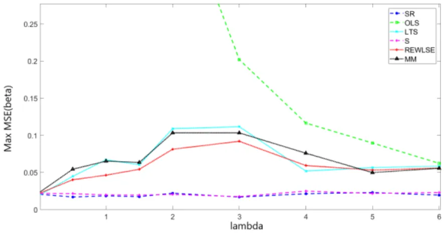
Simulations to study the robustness are carried out, considering the third simulation scheme [NEO]. The most significant results are those consisting on dimensions p = 5,30 with sample sizes n = 100,500, respectively. The two statistical criteria used to compare the estimators from the different approaches were the squared Bias and the MSE for the estimated parameter vector ˆβand for the estimated intercept ˆαaveraging over allM simulation runs (see Gervini and Yohai[2002], Croux et al. [2003], Rousseeuw et al.[2004]). The following figures show, for each value ofλ, the maximal value of MSE or Bias, obtained over all possible values ofk.

M M SEλ(·) =maxk∈{0,...,10}M SEλ,k(·)

M Biasλ(·) =maxk∈{0,...,10}Biasλ,k(·), (19)

for eachλ∈ {0, ...,10}. Figure1shows theM M SE( ˆβ), in case of low dimension p= 5 with sample sizen= 100 and when the data is contaminated with a level of 10%. OLS shows high MSE when the data contains atypical observations, specially for vertical outliers and bad leverage observations associated with the first values ofλ.

Figure 1: M M SE( ˆβ) withp= 5,n= 100, δ= 10%.

If the previous image is zoomed, Figure 2, it can be seen that for vertical outliers, i.e. λ= 0, all robust methods have similar MSE, but for the remaining values of λ, the smallest errors correspond to the proposed method SR and method S.

Figure 2: (Zoom)M M SE( ˆβ) withp= 5,n= 100,δ= 10%.

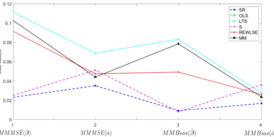
For the MSE of ˆα, and for the Bias of both ˆαand ˆβ, similar conclusions are obtained. In order to see these results from a different perspective, the error measures are summarized in a single graph for each dimension, sample size and contamination level. Figure3corresponds top= 5,n= 100 andδ= 10%. Each line represents a method. In the x-axis each number from 1 to 4 represents the maximum error measures: 1-MMMSE( ˆβ), 2-MMMSE( ˆα), 3-MMBias( ˆβ) and

4-MMBias( ˆα), over all possible values ofλ.

M M M SE(·) =maxλ∈{0,...,10}M M SEλ(·)

M M Bias(·) =maxλ∈{0,...,10}M Biasλ(·), (20) for eachλ∈ {0, ...,10}.

Figure 3: M M M SE, withp= 5,n= 100 andδ= 10%.

Figure4 is a zoom of the previous Figure3. We can see in Figure4that in the majority of cases the proposed method SR has the lowest maximum MSE or Bias, except for one case in which method S has slightly lower maximum Bias( ˆβ), but this happens only under low level of contamination.

Figure 4: (Zoom)M M M SE, withp= 5 andδ= 10%.

When the contamination level δ increases to 20%, method S worsens its performance as it can be seen in Figure5.

Figure 5: M M M SE, withp= 5 andδ= 20%.

Zoomed Figure 6 shows that, in case of higher contamination level, SR is the overall best performance method taking into account that although MSE( ˆα) and Bias( ˆα) are slightly lower for LTS, the MSE and Bias of the ˆβ for LTS is much higher than SR, REWLSE and even MM estimator.

Figure 6: (Zoom)M M M SE, withp= 5 andδ= 20%.

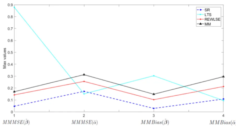
Figure 7 shows that when the dimension is increased to p = 30, and the contamination isδ= 10%, the most affected methods are OLS and S. Method SR is the one that has the lowest maximum value for the MSE and Bias of both βandα.

Figure 7: M M M SE, withp= 30 andδ= 10%.

Figure 8 is a zoom of Figure7 so we can see the four methods with lowest errors. A similar situation happens in case ofδ= 20% of contamination.

Figure 8: (Zoom)M M M SE, withp= 30 andδ= 10%.

In the AppendixA, Tables 1 - 4 have the numerical results, showing for each method the maximum (across λ and k) MSE and Bias for both ˆβ and ˆα for each combination of the dimension p and the contamination level δ. In bold letter are the lowest error and in italic letter are the highest error after OLS. The results bear out with the ones from the Figures.

6.1

Computational times

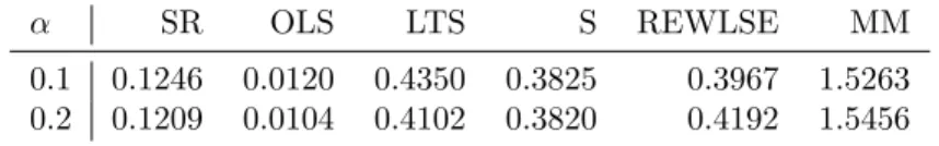
The computational times in seconds for each method in simulation scenario [NEO] are also measured. The study was performed in a PC with a 3.40 GHz Intel Core i7 processor with 32GB RAM. The results are averaged for 10% and 20% of contamination since they were similar. OLS is obviously the fastest one because its simplicity. Following OLS, the proposed method SR is the second fastest method because it does not relies on iterative algorithms to calculate the estimations. The other robust competitors are between 3 and 9 times slower than our proposal SR for low dimension, and between 3 and 12 times slower for higher dimension.

Table 3: Computational times with Normal distributionp= 5 andn= 100

α SR OLS LTS S REWLSE MM

0.1 0.0206 0.0126 0.0989 0.0515 0.0572 0.1816 0.2 0.0200 0.0102 0.0966 0.0514 0.0545 0.1862

Table 4: Computational times with Normal distributionp= 30 andn= 500

α SR OLS LTS S REWLSE MM

0.1 0.1246 0.0120 0.4350 0.3825 0.3967 1.5263 0.2 0.1209 0.0104 0.4102 0.3820 0.4192 1.5456

7

Equivariance properties

The initial shrinkage robust estimators ˆµ_Shand ˆΣShare approximately affine equivariant (Cabana et al.[2019]). This means that the equivariance property cannot be demonstrated analytically because only part of the property holds, but it can be studied by means of simulations (as inMaronna and Zamar[2002] andSajesh and Srinivasan [2012]). Then, the distance defined in Equation 10 and used in the weights for the SW estimators of mean and covariance matrix (Equation 11) remains approximately invariant under affine transformations. Since the weights are hard rejection depending on the robust distance, the esti-mators ˆµSWSh and ˆΣSWSh should hold the property. However, the real interest in the regression problem is concerned around the parameter estimators, denoted as: ˆϕSR = ˆ βSR t ,αˆSR t

. Thus, we propose to study the equivariance property on them. Affine equivariance in regression can be split in the three following properties (Rousseeuw et al. [2004] and Maronna and Morgenthaler

[1986]):

1. Regression equivariance: If a linear function of the explanatory vari-ables is added to the response, then the coefficients of this linear function

are also added to the estimators.

2. y-equivariance: If the response variable is transformed linearly then the estimators transforms correctly.

Property (1) and (2) can be seen together as: ˆ

ϕSR(X,yc+Xg+v) = ˆϕSR(X,y)c+ (gt, v)t, (21) wherec∈_Ris any non-singular constant,gis anyp×1 vector andv∈_R is any constant. This means that, keeping the sameX, and transforming the response as yc+Xg+v, the resulting transformed estimators are: ˆ

βSR_new=c( ˆβSR) +gand ˆαSR

new=cαˆSR+v.

3. x-equivariance: Also called carrier equivariance. It says that if the explanatory variables are transformed linearly (coordinate system trans-formation), then the estimators transforms correctly.

ˆ

ϕSR(XA,y) = (( ˆβSR)t(A−1)t,αˆSR)t. (22) This means that if the carriers are transformed as XA with any non-singular p×p matrixA, the resulting estimators are: ˆβSR_new = A−1_βˆSR and the intercept should remain the same ˆαSR

new= ˆαSR.

Exploring all possible transformations is infeasible, that is the reason why

Maronna and Zamar[2002] and Sajesh and Srinivasan[2012] proposed to gen-erate the random matricesAfor thex-equivarianceasA=T D, whereT is a random orthogonal matrix andD=diag(u1, ..., up), where theuj’s are indepen-dent and uniformly distributed in (0,1), for allj= 1, ..., p. Then, each generated data matrixX in each repetition, is transformed with a random transformation A. Following this idea, we propose to generate the non-singular c, the g and thev for regression andy-equivariance, randomly for each repetition.

The MSE of the proposed method SR is studied when the transformations described above are made to the simulated data-set. Consider the simulation scenario [NE] for normal data without outliers (δ = 0%) and scenario [NEO] when there isδ= 10%,20% of contamination, to see the impact of the presence of outliers. The vector of regression parameters ˆϕSR is estimated with the untransformed data and saved. After that, the data is transformed according to Equation21for the regression andy-equivariance and according to Equation22 for thex-equivariance. Next, the method SR is applied to the transformed data and the resulting ˆϕSRneware saved. The MSE is calculated between the obtained

ˆ

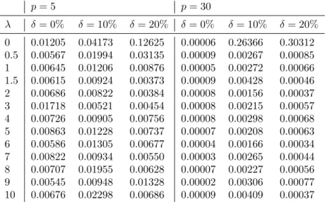
ϕSRnewand what it should be obtained if the equivariance properties hold. Table 5shows for each λ, the resulting M M SEλ( ˆϕSRnew).

Table 5: M M SEλ( ˆϕSR_new) for regression andy-equivariance p= 5 p= 30 λ δ= 0% δ= 10% δ= 20% δ= 0% δ= 10% δ= 20% 0 0.01205 0.04173 0.12625 0.00006 0.26366 0.30312 0.5 0.00567 0.01994 0.03135 0.00009 0.00267 0.00085 1 0.00645 0.01206 0.00876 0.00005 0.00272 0.00066 1.5 0.00615 0.00924 0.00373 0.00009 0.00428 0.00046 2 0.00686 0.00822 0.00384 0.00008 0.00156 0.00037 3 0.01718 0.00521 0.00454 0.00008 0.00215 0.00057 4 0.00726 0.00905 0.00756 0.00008 0.00298 0.00068 5 0.00863 0.01228 0.00737 0.00007 0.00208 0.00063 6 0.00586 0.01305 0.00677 0.00004 0.00166 0.00034 7 0.00822 0.00934 0.00550 0.00003 0.00265 0.00044 8 0.00707 0.01955 0.00628 0.00007 0.00227 0.00056 9 0.00545 0.00948 0.01328 0.00002 0.00306 0.00077 10 0.00676 0.02298 0.00686 0.00009 0.00409 0.00037 For vertical outliers, i.e. whenλ= 0, the error increases with the increase in dimension and contamination level, a fact that is influenced mostly by the error of the intercept. Nevertheless, for the rest of the cases the maximum possible error is low. Table6 shows the results for thex-equivariance. In this case, both for vertical outliers and leverage points, the error remains low. Thus, since the errors are mostly controlled, the proposed robust regression estimator is approximately regression, y- and x-equivariant.

Table 6: M M SEλ( ˆϕ SR

new) forx-equivariance p= 5 p= 30 λ δ= 0% δ= 10% δ= 20% δ= 0% δ= 10% δ= 20% 0 0.00206 0.00421 0.01874 0.00005 0.01324 0.09468 0.5 0.00162 0.00456 0.01310 0.00003 0.00026 0.00008 1 0.00178 0.00348 0.00493 0.00003 0.00030 0.00003 1.5 0.00153 0.00392 0.00132 0.00004 0.00012 0.00006 2 0.00198 0.00320 0.00234 0.00003 0.00034 0.00003 3 0.00144 0.00293 0.00208 0.00003 0.00016 0.00002 4 0.00177 0.00329 0.00359 0.00005 0.00026 0.00005 5 0.00194 0.00339 0.00182 0.00003 0.00020 0.00001 6 0.00173 0.00481 0.00205 0.00005 0.00016 0.00002 7 0.00214 0.00329 0.00184 0.00002 0.00012 0.00002 8 0.00186 0.00415 0.00177 0.00004 0.00013 0.00002 9 0.00242 0.00356 0.00188 0.00004 0.00016 0.00001 10 0.00193 0.00287 0.00250 0.00003 0.00011 0.00001

8

Breakdown property

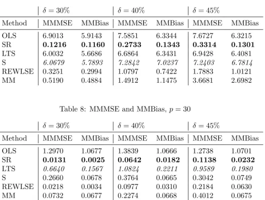
The bdp measures the maximum proportion of outliers that the estimator can safely tolerate. The highest possible value for the bdp is 50%. The empir-ical breakdown value can be examined through simulations, as in Sajesh and Srinivasan [2012], considering high contamination levels. Although these sit-uations are not that relevant in practice because low levels of contamination should be expected, we propose to study if the error and the bias are controlled in these scenarios in order to see the performance of the proposed SR estimator. For this, [NEO] contamination scheme is used, but considering higher levels of contaminationsδ= 30%,40%,45%. Table7 shows the resulting MMMSE and MMBias for ˆϕSR_new in the low dimensionp= 5 case.

Table 7: MMMSE and MMBias,p= 5

δ= 30% δ= 40% δ= 45%

Method MMMSE MMBias MMMSE MMBias MMMSE MMBias

OLS 6.9013 5.9143 7.5851 6.3344 7.6727 6.3215 SR 0.1216 0.1160 0.2733 0.1343 0.3314 0.1301 LTS 6.0032 5.6686 6.6864 6.3431 6.9428 6.4081 S 6.0679 5.7893 7.2842 7.0237 7.2403 6.7814 REWLSE 0.3251 0.2994 1.0797 0.7422 1.7883 1.0121 MM 0.5190 0.4884 1.4912 1.1475 3.6681 2.6982

Table 8: MMMSE and MMBias,p= 30

δ= 30% δ= 40% δ= 45%

Method MMMSE MMBias MMMSE MMBias MMMSE MMBias

OLS 1.2970 1.0677 1.3839 1.0666 1.2738 1.0701 SR 0.0131 0.0025 0.0642 0.0182 0.1138 0.0232 LTS 0.6640 0.1567 1.0824 0.2211 0.9589 0.1980 S 0.2660 0.0678 0.3764 0.0665 0.3042 0.0749 REWLSE 0.0218 0.0034 0.0977 0.0310 0.2184 0.0630 MM 0.0732 0.0677 0.2274 0.0668 0.4012 0.0675

Table8shows the results for higher dimensionp= 30. Bold letter represents lower error or bias and italic letter represents the highest measures after OLS, which is the method with worse results. LTS, S and MM have high error and bias for both low and high dimension, specially with the increase of the con-tamination level. REWLSE is competitive with SR in high dimension, but in low dimension REWLSE shows higher errors. The MSE and Bias of SR remain low, specially in high dimension and even with large contamination in the data, compared with the other robust methods supposedly having a high bdp. As

discussed in Yu and Yao [2017] where the authors review and compare some robust regression approaches, the issue here is that although LTS, S and MM have high bdp, the computation is very challenging (Hawkins and Olive[2002] and Stromberg et al. [2000]). That is why resampling algorithms are used to obtain a number of subsets and then compute the robust regression estimate from a number of initial estimates. However, the high breakdown property usu-ally requires that the number of elementary sets goes to infinity, for example,

Hawkins and Olive[2002] proved that LTS computed with fast-LTS algorithm had zero bdp. In order to compute these estimators with high bdp, one should consider all possible elemental sets. SR approach shows high resistance to large contamination even in high dimension, which can be translated in high empirical bdp.

9

Real examples

In this section, we study two known data-sets, very often used in the liter-ature, to illustrate the performance of the proposed robust regression method comparing to the other robust alternatives. And also a socioeconomic and en-vironmental related data-set that explains the Living Environment Deprivation of areas of Liverpool through remote-sensed data obtained from Google Earth technologies (Arribas-Bel et al.[2017]).

9.1

Star data

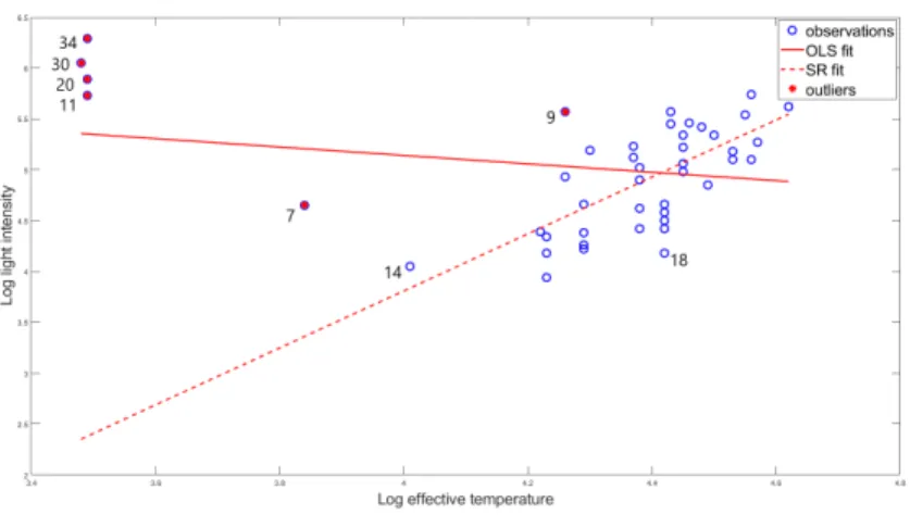
The first example is the star data-set, and it is reported in Leroy and Rousseeuw[1987], and based onHumphreys[1978] andDe Gr`eve and Vanbev-eren[1980]. It has become a bench-mark for robust regression methodologies. It consists onn= 47 observations corresponding to 47 stars of the CYG OB1 clus-ter in the direction of Cygnus. There is only one carrierxwhich is the logarithm of the effective temperature at the surface of the star. The response variable y is the logarithm of its light intensity. There is a positive linear relationship between the response and the explanatory variables, except for four red giant stars (observations 11, 20, 30 and 34) which are outliers because they have low temperatures and a high output of light (the four observations on the upper left corner in Figure9). These giant stars actually represent a different population. They are bad leverage points because they influence OLS regression line due to the poor estimation of the parameters. Figure9shows how the four giant stars pull the OLS line towards them. Observations 7 and 9 are intermediate outliers. And finally, in the multivariate sense, observation 14 is often detected as outlier, but in the regression sense it is a good leverage point because it follows the same linear pattern than the bulk data. Robust regression fit made by the proposed method SR detected the giant stars 11, 20, 30, 34 and the intermediate outliers 7 and 9.

Table9 summarizes all method’s estimation of the intercept and slope, and the outliers detected by the robust methods. Note that OLS estimates are

Figure 9: Star data-set with OLS and SR regression fit.

completely changed, they have even different sign. SR and REWLSE correctly detect the regression outliers, method S detects the good leverage point, obser-vation 14, as an outlier. LTS detects obserobser-vation 18 as atypical when it is not. In Figure 9 it can be seen that observation 18 is an example of the swamping effect problem. On the other hand, MM approach only detects as outliers the giant stars (masking effect).

Table 9: Estimation of intercept and slope and detected outliers with star data. Method αˆ βˆ Detected outliers

OLS 6.7935 -0.4133 SR -7.4035 2.9028 7 9 11 20 30 34 LTS -8.5001 3.0462 7 9 11 18 20 30 34 S -10.5034 3.4994 7 9 11 14 20 30 34 REWLSE -7.5001 3.0462 7 9 11 20 30 34 MM -5.1234 2.2879 11 20 30 34

The R2 values for the linear regression models fitted by each method are summarized in Table10. OLS’s coefficient of determination is low, while that of the robust methods is high, except for MM approach which is lower than the rest.

Table 10: R2 _{for each method with stars data-set.}

Method OLS SR LTS S REWLSE MM R2 0.0443 0.7113 0.7006 0.7035 0.7095 0.5578

9.2

Hawkins-Bradu-Kass data

HBK data-set was artificially created by Hawkins et al. [1984] and it was also used inLeroy and Rousseeuw[1987], and many others. It containsp= 3 explanatory variables and a response variable. The first 14 observations are leverage points: 1-10 of bad type and 11-14 of good type. Thus, only observa-tions 1-10 are outliers in the regression sense. Table11 shows the estimation by all methods for the three parameters, and it can be seen that OLS is highly influenced by the presence of these leverage points. Also, the parameter esti-mated by S method are different than that of the other robust approaches, and the reason for this is that all robust methods correctly detect the true outliers, except for method S, which also includes the good leverage points 11-14.

Table 11: Estimation of the parameters and detected outliers with HBK data. Method βˆ0 βˆ1 βˆ2 βˆ3 Detected outliers

OLS -0.3875 0.2392 -0.3345 0.3833 SR -0.1800 0.0836 0.0396 -0.0518 1 2 3 4 5 6 7 8 9 10 LTS -0.1805 0.0814 0.0399 -0.0517 1 2 3 4 5 6 7 8 9 10 S -0.0174 0.0957 0.0041 -0.1286 1 2 3 4 5 6 7 8 9 10 11 12 13 14 REWLSE -0.1805 0.0814 0.0399 -0.0517 1 2 3 4 5 6 7 8 9 10 MM -0.1913 0.0860 0.0412 -0.0541 1 2 3 4 5 6 7 8 9 10 The adjustedR2_{values are summarized in Table12. Here, all robust} meth-ods, except S, have high and similarR2_.

Table 12: AdjustedR2 _{for each method with HBK data-set.} Method OLS SR LTS S REWLSE MM

R2 _{0.5850 0.9818 0.9816 0.9002 0.9817 0.9811}

9.3

Living Environment Deprivation data

In Arribas-Bel et al. [2017], the authors studied the Living Environment Deprivation (LED) index. This measure allows to study quantitatively the concept of quality of the local environment, known also as urban quality of life, which is a qualitative concept. This is an essential matter for environmental research, citizens and politics. This kind of indices can be explained through remote sensing data, i.e. information collected without making physical contact, for example, from satellite technologies. The authors inArribas-Bel et al.[2017] proposed to model the LED index of Liverpool (UK) based on four sets of explanatory variables extracted from a very high spatial resolution (VHR) image downloaded from Google Earth. The four groups are called: land cover (LC), spectral (SP), texture (TX) and structure features (ST). SeeArribas-Bel et al.

to explain the LED index with a linear combination of the four sets of variables. The linear regression model is the following:

LED=α+βLC+γSP+δT X+ζST+ . (23) There are 35 explanatory variables,β,γ,δandζare vectors, containing the parameters for each carrier, andis an error term assumed to be i.i.d. follow-ing a Gaussian distribution. The classical approach to estimate the regression parameters is using Ordinary Least Squares (OLS). The problem here is that the way of acquisition of the data, which is obtaing features from processing images from satellite technology, may imply the presence of atypical observa-tions that could invalidate the results. Therefore, robust methodologies need to be used. On the other hand, the large number of variables derived from the Google Earth image, particularly those of spectral, texture and structure types, are substantially correlated (Figure10).

Figure 10: Correlation matrix for LED index data-set.

The multicollinearity issue violates another assumption for using OLS to esti-mate the parameters of the model. The authors propose to use a dimensionality-reduction step to preserve as much of the variation contained in the entire set of variables while eliminating collinearity. They performed a principal compo-nents analysis (pca) (Jolliffe [2011]) on all the spectral, texture and structure variables, which makes a total of 27 variables, and after the analysis they pro-pose to use only the first four components because they accounted for 90% of the total variance. The four extracted components were used as regressors, together with the three land cover variables that prove most relevant: water, shadow, and vegetation. They came up with this result about the relevance by using another approach, but from machine learning area, which is the random forest (RF), since one of the main objectives of the paper was to study the potential of

modern machine learning techniques: RF and gradient boost regressor (GBR), in the estimation of socioeconomic indices with remote-sensing data. Focusing on the classical OLS regression, the authors obtained that the third and fourth components were significant, as well as the proportion of an area occupied by water and vegetation.

We propose to study if the results can be improved by using robust regres-sion methods. Let us apply the proposed SR approach and compare it with LTS, S, REWLSE and MM. The raw data, kindly provided by the authors was pre-processed the same way as they propose, by applying pca to the last 27 ex-planatory variables and join the first four components with the three land cover variables: water, shadow and vegetation, which makes a total of 7 explanatory variables. Table 13 shows the adjusted R2 _{of the models estimated by each} method.

Table 13: R2 _{with (pca transformed) LED index data-set.} Method OLS SR LTS S REWLSE MM

R2 _{0.5059 0.6716 0.6287 0.6031 0.5904 0.6166} Variables PC3, PC4, water and vegetation resulted significant in the model obtained by the methods. The percentage of variability explained by the robust methods shows the advantage of robust regression. TheR2of SR is higher than that of the other approaches, although not as high as one would wish. The authors compare the results from OLS with the application of the two machine learning approaches. RF showed an R2 _{= 0.9354 and GBR anR}2 _{= 0.8320.} They were interested in finding the best possible model with the ability of capture as much proportion of the variation inherent in the data as possible. But the problem here is the drawback both machine learning methods have in terms of interpretability. Also, as the authors point out, RF and GBR suffer from the issue of overfitting. That is why they propose a cross validation (CV) study. It consisted on dividing the data in two groups, one to train the model, and the other one to test its predictive performance. The 5-fold CV was used and the procedure was repeated 250 times, to obtain the scores for theR2_{, as} in the paper. The scores for the MSE of the response are also saved. Table14 shows the median cross-validatedR2 obtained by the authors for RF and GBR together with the one we obtained for method SR.

Table 14: Median cross-validatedR2 _{with (pca transformed) LED index} data-set.

Method SR RF GBR

R2 _{0.6704 0.54 0.50}

The results show that SR is more robust to overfitting since theR2is reduced slightly, while that of RF and GBR are significantly reduced. Between the

three values, SR has the highest median cross-validatedR2. On the other hand, for method SR, the median absolute deviation from the data’s median (MAD) of these scores is 0.0145 which is low, meaning that the uncertainty is under control. Figure11(a)shows the distribution of the cross-validated scores for the R2 obtained with method SR and the median value in a dashed line.

(a) Cross-validatedR2 _{(b) Cross-validated MSE} Figure 11: CV scores and median values (dashed line), with pca. Figure 11(b) shows the results for the MSE. The median of the cross-validated MSE is equal to 2.6260 and the MAD is 0.1199 which are also low values.

Since it was mentioned before, the same pca transformation the authors proposed for the data was made for this research. Now, we propose another transformation that improves the performance according to the results: sparse pca (spca) (Zou et al. [2006]), which has advantages in case of high correlated variables since it is a kind of variable selection transformation. The spca was made over the 27 variables of the three last groups and the first 10 components were selected since they account for 92.04% of the total variance. These 10 components and the three most relevant land cover variables: water, shadow and vegetation were used to estimate the model.

Figure12(a)shows the distribution of the cross-validatedR2and the median value in a dashed line obtained with SR, which is 0.8530. The MAD of these scores increases to 0.0346 but it is still a low value. Figure 12(b) shows the distribution for the MSE. The median MSE reduces to 0.7244 and the MAD reduces to 0.0177.

(a) Cross-validatedR2 _{(b) Cross-validated MSE} Figure 12: CV measures and median values (dashed line), with spca. Table 15shows that the median cross-validated R2 _{is higher than that} ob-tained with pca transformation but also higher than the obob-tained with both machine learning techniques, reported inArribas-Bel et al.[2017].

Table 15: Median cross-validatedR2. Method SR spca SR pca RF GBR

R2 _{0.8530 0.6704 0.54 0.50}

The uncertainty of the obtainedR2 _{is slightly higher with spca} transforma-tion, compared to that with the pca transformation. But Figure13shows that the distributions of theR2 _{scores are quite separated, and the gain is obvious} because of the increase in the median value.

Figure 13: Cross-validated R2 and median values (dashed line), for both pca and spca.

Finally, Table16contains the estimated coefficients, the p-values and theR2 estimated by SR with spca transformation using the complete data-set, which is competitive with respect to theR2 of RF and GBR reported in Arribas-Bel et al.[2017]. As the results point out, the same land cover variables as in the paper remained significant and with the same negative sign, meaning that larger proportions of water and vegetation are associated with smaller deprivation. Table 16: Results for the model estimated by SR with spca transformation and theR2 _{for RF and GBR.}

coefficient p-value RF GBR constant 0.27191 2.03E-05 water -1.42641 2.00E-16 vegetation -0.44513 2.00E-05 SPC2 -0.04409 4.51E-03 SPC3 0.13215 1.52E-06 SPC4 0.32566 1.03E-15 SPC5 -0.26745 2.35E-11 SPC7 -0.13735 2.24E-03 SPC8 0.19544 1.64E-03 R2 0.86820 0.9354 0.8320

10

Conclusions

In the paper, the performance of the proposed SR approach is compared to the classical OLS and other existing robust regression methods. The robust al-ternatives in the literature have some drawbacks and their performance depend on decisions that, in case of real data, increase the difficulty of robustly estimate the regression parameters. On the other hand, not all available methods have a good behavior in case of large data-sets, high dimension, not all are scalable in terms of computational time, proven to be sufficiently resistant to the presence of outliers. The proposal in this paper is to use the notion ofshrinkage in order to define robust estimators of location and scatter to estimate the regression pa-rameters. The approach passes through a pair of weighting steps depending on robust Mahalanobis distances, which results in the shrinkage reweighted (SR) regression estimator. The advantages of using the shrinkage are shown in the simulation study and some conclusions can be noted. SR approach yielded com-petitive results compared to the alternative robust methods from the literature for the regression problem, even in high dimension, heavy-tailed distributed er-rors, large contamination or transformed data. Furthermore, SR is quite stable computationally since it involves contributions from all the observations instead of sub-sample iterations from the data. Finally, the results with the real data-set examples bear out with the conclusions from the simulation study. Specially with the LED index data where the SR approach provides an improvement of the

cross-validatedR2and MSE with respect to classical OLS and machine learning techniques RF and GBR, while maintaining the advantage of interpretability. It remains to be examined as future research if the proposal could be improved by using adjusted quantiles instead of the classical choices from the literatureq1 andq2 from Equation16, which are derived from the chi-squared distribution.

11

Acknowledgments

This research was partially supported by MINISTERIO DE ECONOMIA, INDUSTRIA Y COMPETITIVIDAD, award number: ECO2015-66593-P.

A

Appendix

Tables 17 - 20 show the numerical results for Section 6 Robustness of the paper, in simulation scheme [NEO]. For each method, the maximum (across λ andk) MSE and Bias for both ˆβand ˆαfor each combination of the dimension pand the contamination levelδ, is showed. In bold letter are the lowest error and in italic letter are the highest error after OLS.

Table 17: MMMSE and MMBias of ˆβand ˆα, forp= 5 and δ= 10%.

Method

MSE( ˆ

β

)

MSE( ˆ

α)

BIAS( ˆ

β

)

BIAS( ˆ

α)

OLS

2.9065

5.5593

2.7004

5.3280

SR

0.0230

0.0351

0.0093

0.0168

LTS

0.1116

0.0688

0.0832

0.0275

S

0.0249

0.0512

0.0083

0.0361

REWLSE

0.0919

0.0474

0.0493

0.0260

MM

0.1033

0.0441

0.0785

0.0235

Table 18: MMMSE and MMBias of ˆβand ˆα, forp= 5 and δ= 20%.

Method

MSE( ˆ

β

)

MSE( ˆ

α)

BIAS( ˆ

β

)

BIAS( ˆ

α)

OLS

3.7360

29.9723

3.6101

29.4112

SR

0.0470

0.1720

0.0287

0.1075

LTS

0.8779

0.1508

0.3028

0.0947

S

1.3853

5.4441

0.6577

3.8112

REWLSE

0.1422

0.2556

0.1018

0.2124

MM

0.1688

0.3120

0.1478

0.2954

Table 19: MMMSE and MMBias of ˆβand ˆα, forp= 30 andδ= 10%.

Method

MSE( ˆ

β

)

MSE( ˆ

α

)

BIAS( ˆ

β

)

BIAS( ˆ

α

)

OLS

0.1995

6.7748

0.0610

6.7250

SR

0.0033

0.0101

0.0009

0.0030

LTS

0.0139

0.0145

0.0102

0.0060

S

0.1079

2.9888

0.0584

2,9439

REWLSE

0.0077

0.0165

0.0070

0.0080

MM

0.0120

0.0134

0.0101

0.0116

Table 20: MMMSE and MMBias of ˆβand ˆα, forp= 30 andδ= 20%.

Method

MSE( ˆ

β

)

MSE( ˆ

α

)

BIAS( ˆ

β

)

BIAS( ˆ

α

)

OLS

0.2317

25.5388

0.0639

25.3395

SR

0.0044

0.0596

0.0011

0.0554

LTS

0.0450

0.3952

0.0400

0.3677

S

0.1710

15.0446

0.0635

14.8378

REWLSE

0.0120

0.0980

0.0017

0.0930

MM

0.0356

0.1994

0.0262

0.1860

References

J. Agull´o, C. Croux, and S. Van Aelst. The multivariate least-trimmed squares estimator. Journal of Multivariate Analysis, 99(3):311–338, 2008.

D. Arribas-Bel, J. E. Patino, and J. C. Duque. Remote sensing-based mea-surement of Living Environment Deprivation: Improving classical approaches with machine learning. PLOS ONE, 12(5):e0176684, 2017.

E. Cabana, R. E. Lillo, and H. Laniado. Multivariate outlier detection based on a robust Mahalanobis distance with shrinkage estimators. 2019. URL

http://arxiv.org/abs/1904.02596.

C. Croux, P. J. Rousseeuw, and O. H¨ossjer. Generalized S-Estimators. Journal of the American Statistical Association, 89(428):1271, 1994.

C. Croux, S. Van Aelst, and C. Dehon. Bounded influence regression using high breakdown scatter matrices. Annals of the Institute of Statistical Mathemat-ics, 55(2):265–285, 2003.

D. D’Alimonte and D. Cornford. Outlier detection with partial information: application to emergency mapping. Stochastic Environmental Research and Risk Assessment, 22(5):613–620, 2008.

J. P. De Gr`eve and D. Vanbeveren. Close binary systems before and after mass transfer: A comparison of observations and theory. Astrophysics and Space Science, 68(2):433–457, 1980.

V. DeMiguel, A. Martin-Utrera, and F. J. Nogales. Size matters: Optimal calibration of shrinkage estimators for portfolio selection.Journal of Banking & Finance, 37(8):3018–3034, 2013.

D. L. Donoho and P. J. Huber. The notion of breakdown point. InA festschrift for Erich L. Lehmann, volume 157184. 1983.

F. Y. Edgeworth. On observations relating to several quantities. Hermathena, 6:279–285, 1887.

M. Falk. On Mad and Comedians. Annals of the Institute of Statistical Mathe-matics, 49(4):615–644, 1997.

D. Gervini and V. J. Yohai. A class of robust and fully efficient regression estimators. The Annals of Statistics, 30(2):583–616, 2002.

D. M. Hawkins and D. J. Olive. Inconsistency of Resampling Algorithms for High-Breakdown Regression Estimators and a New Algorithm.Journal of the American Statistical Association, 97(457):136–148, 2002.

D. M. Hawkins, D. Bradu, and G. V. Kass. Location of Several Outliers in Multiple-Regression Data Using Elemental Sets. Technometrics, 26(3):197, 1984.

P. J. Huber. Robust Estimation of a Location Parameter.The Annals of Math-ematical Statistics, 35(1):73–101, 1964.

P. J. Huber. Robust Regression: Asymptotics, Conjectures and Monte Carlo. The Annals of Statistics, 1(5):799–821, 1973.

P. J. Huber. Robust statistics. New York John Wiley and Sons, 1981.

R. M. Humphreys. Studies of luminous stars in nearby galaxies. I. Supergiants and O stars in the Milky Way. The Astrophysical Journal Supplement Series, 38:309, 1978.

W. James and C. Stein. Estimation with Quadratic Loss. InBreakthroughs in statistics, pages 443–460. Springer, New York, NY, 1992.

D. Jeong, A. St-Hilaire, T. Ouarda, and P. Gachon. Comparison of transfer functions in statistical downscaling models for daily temperature and precip-itation over canada. Stochastic environmental research and risk assessment, 26(5):633–653, 2012.

I. Jolliffe. Principal Component Analysis. In International Encyclopedia of Statistical Science, pages 1094–1096. Springer Berlin Heidelberg, Berlin, Hei-delberg, 2011.

O. Ledoit and M. Wolf. Improved estimation of the covariance matrix of stock returns with an application to portfolio selection. Journal of Empirical Fi-nance, 10(5):603–621, 2003a.

O. Ledoit and M. Wolf. A well-conditioned estimator for large-dimensional covariance matrices. Journal of Multivariate Analysis, 88(2):365–411, 2004. O. Ledoit and M. N. Wolf. Honey, I Shrunk the Sample Covariance Matrix.

UPF Economics and Business Working Paper No. 691, 2003b.

A. M. Leroy and P. J. Rousseeuw.Robust regression and outlier detection. 1987. H. P. Lopuhaa and P. J. Rousseeuw. Breakdown points of affine equivariant estimators of multivariate location and covariance matrices. The Annals of Statistics, 19(1):229–248, 1991.

R. Maronna and S. Morgenthaler. Robust regression through robust covariances. Communications in Statistics - Theory and Methods, 15(4):1347–1365, 1986. R. A. Maronna and R. H. Zamar. Robust Estimates of Location and Dispersion

for High-Dimensional Datasets. Technometrics, 44(4):307–317, 2002.

R. A. Maronna, R. D. Martin, and V. J. Yohai. Robust statistics : theory and methods. John Wiley & Sons, 2006.

H. Mourino and M. I. Barao. A comparison between the linear regression model with autocorrelated errors and the partial adjustment model. Stochastic En-vironmental Research and Risk Assessment, 24(4):499–511, 2010.

H. Oja. Multivariate nonparametric methods with R : an approach based on spatial signs and ranks. Springer, 2010.

Z. Pan, P. Liu, S. Gao, M. Feng, and Y. Zhang. Evaluation of flood season segmentation using seasonal exceedance probability measurement after outlier identification in the three gorges reservoir. Stochastic environmental research and risk assessment, pages 1–14, 2018.

M. Riani, D. Perrotta, and F. Torti. FSDA: A MATLAB toolbox for robust analysis and interactive data exploration.Chemometrics and Intelligent Lab-oratory Systems, 116:17–32, 2012.

P. Rousseeuw and V. Yohai. Robust Regression by Means of S-Estimators. pages 256–272. Springer, New York, NY, 1984.

P. J. Rousseeuw. Multivariate estimation with high breakdown point. Mathe-matical statistics and applications, 8:287–297, 1983.

P. J. Rousseeuw. Least Median of Squares Regression. Journal of the American Statistical Association, 79(388):871–880, 1984.

P. J. Rousseeuw and C. Croux. Alternatives to the Median Absolute Deviation. Journal of the American Statistical Association, 88(424):1273, 1993.

P. J. Rousseeuw, S. V. Aelst, K. Van Driessen, and J. Agull´o. Robust Multi-variate Regression. 2004.

D. Ruppert. Computing S Estimators for Regression and Multivariate Loca-tion/Dispersion. Journal of Computational and Graphical Statistics, 1(3): 253, 1992.

T. A. Sajesh and M. R. Srinivasan. Outlier detection for high dimensional data using the Comedian approach. Journal of Statistical Computation and Simulation, 82(5):745–757, 2012.

C. Sguera, P. Galeano, and R. E. Lillo. Functional outlier detection by a local depth with application to no x levels. Stochastic environmental research and risk assessment, 30(4):1115–1130, 2016.

A. F. Siegel. Robust Regression Using Repeated Medians. Biometrika, 69(1): 242, 1982.

A. J. Stromberg, O. H¨ossjer, and D. M. Hawkins. The Least Trimmed Dif-ferences Regression Estimator and Alternatives. Journal of the American Statistical Association, 95(451):853–864, 2000.

Y. Tung, K. Yeh, and J. Yang. Regionalization of unit hydrograph parameters: 1. Comparison of regression analysis techniques, 11:17, 1997.

Y. Vardi and C. H. Zhang. The multivariate L1-median and associated data depth. Proceedings of the National Academy of Sciences of the United States of America, 97(4):1423–6, 2000.

S. Verboven and M. Hubert. LIBRA: a MATLAB library for robust analysis. Chemometrics and Intelligent Laboratory Systems, 75(2):127–136, 2005. V. J. Yohai. High Breakdown-Point and High Efficiency Robust Estimates for

Regression. The Annals of Statistics, 15(2):642–656, 1987.

C. Yu and W. Yao. Robust linear regression: A review and comparison. Com-munications in Statistics - Simulation and Computation, 46(8):6261–6282, 2017.

H. Zou, T. Hastie, and R. Tibshirani. Sparse Principal Component Analysis. Journal of Computational and Graphical Statistics, 15(2):265–286, 2006.