Data fusion of radar and stereo vision for detection and tracking of moving objects

(1)

Detection and Tracking of Moving Objects

by

Frik Botha

Thesis presented in partial fulfilment of the requirements for

the degree of Master of Engineering (Electronic) in the

Faculty of Engineering at Stellenbosch University

Department of Electrical and Electronic Engineering, University of Stellenbosch,

Private Bag X1, Matieland 7602, South Africa.

Supervisors:

Dr C. E. van Daalen, Mr J. Treurnicht

(2)

Declaration

By submitting this thesis electronically, I declare that the entirety of the work contained therein is my own, original work, that I am the sole author thereof (save to the extent explicitly otherwise stated), that reproduction and publication thereof by Stellenbosch University will not infringe any third party rights and that I have not previously in its entirety or in part submitted it for obtaining any qualification.

Date: ... March 2017 ...

(3)

Abstract

Detection and tracking of moving objects (DATMO) is essential for autonomous navi-gation systems operating in general environments. Dynamic objects must be identified, localised, and their future positions predicted to assist in decision making regarding path planning and collision avoidance. In addition to its application in autonomous navigation, DATMO also forms the basis of various advanced driver assistance systems (ADASs) that are aimed at making road travel more safe. The research presented in this thesis focuses on the combined use of radar and stereo vision for DATMO. The combination of infor-mation from multiple sensors, known as data fusion, introduces redundancy, potentially increasing the confidence and robustness of the system as a whole.

The traditional approach to DATMO is adopted, which involves the chronological steps of measurement extraction, data association and filtering. Measurements are extracted from the radar and vision subsystems independently, using two-dimensional Fourier analy-sis and sparse feature tracking respectively. A segmentation of moving objects is obtained by a track-to-track fusion algorithm, on data composed of image feature track clusters and Gaussian mixtures originating from radar-based state estimation. Segmented objects are ultimately tracked in a novel implementation of the Gaussian inverse Wishart probability hypothesis density (GIW-PHD) filter that makes explicit provision for extended targets, i.e. targets that generate more than one measurements per time step.

Simulation results indicate significantly improved performance for the proposed data fusion algorithm compared to the case when only vision data is used, due to its increased robustness toward clutter interference. Tests on real-world data do not provide conclu-sive evidence that suggests improved performance of the proposed radar-vision fusion algorithm compared to vision-only processing. However, practical limitations meant that truly representative datasets could not be gathered. The practical results, however, do indicate very accurate centre point tracking using the GIW-PHD filter, which attests the effectiveness of the Gaussian inverse Wishart model. Moreover, target extent estimates that result from Gaussian inverse Wishart modelling proves sufficiently accurate for the representation of object extent. GIW-PHD filtering also brings about a consistent in-crease in performance compared to the raw measurements, thereby reinforcing the value of state estimation.

(4)

Uittreksel

Deteksie en volging van bewegende voorwerpe is noodsaaklik vir outonome navigasie stelsels wat in algemene omgewings funksioneer. Bewegende voorwerpe moet ondermeer geïdentifiseer en gelokaliseer word. Terselfdetyd moet voorspellings gemaak word oor sulke voorwerpe se toekomstige beweging om besluitneming in verband met padbeplan-ning en botsingvermeiding by te staan. Benewens die toepassing met betrekking tot out-onome navigasie vorm deteksie en volging van bewegende voorwerpe die basis van verskeie gevorderde bestuurdersbystand stelsels. Die navorsing wat in hierdie verslag voorgelewer word fokus op die gesamentlike gebruik van radar en stereo visie vir deteksie en volging van bewegende voorwerpe. Die kombinasie van inligting vanaf verskeie sensore, bekend as data fusie, bring oorbodige inligting teweeg, met die die potensiaal om die algehele gehalte van die stelsel te verbeter.

Die tradisionele benadering tot deteksie en volging van bewegende voorwerpe word toegepas, wat die kronologiese stappe van meting ontrekking, data assosiasie en afskatting behels. Metings word onafhanklik onttrek vir beide die radar en visie substelsels, deur ge-bruik te maak van twee-dimensionele Fourier analise en yl kenmerk volging respektiewelik. ’n Segmentering van bewegende voorpwerpe word verkry deur middel van ’n toestands-fusie algoritme, wat toegepas word op data bestaande uit groepe beeld kenmerke en radar toestande wat volg uit afskatting. Segmenteerde voorwerpe word uiteindelik gevolg in ’n nuwe implementering van die Gaussies inverse Wishart waarskynlikheidshipotese digth-eid afskatter, wat eksplisiet voorsiening maak vir uitgebrdigth-eide teikens, dit is, teikens wat aanleiding gee tot meer as een meting per tydstap.

Simulasie resultate dui op ’n beduidende verbetering in die prestasie van die voorgestelde data fusie algoritme in vergelyking met die geval waar slegs stereo visie inligting gebruik word, aangesien die metode beter vaar in die teenwoordigheid van steurnisbronne. Toetse op praktiese data gee nie beslissende bewyse om aan te dui dat data fusie beter vaar as die geval waar slegs stereo visie inligting gebruik word nie. Omvattende datastelle kon egter nie ingesamel word nie weens praktiese beperkings. Die praktiese resultate dui egter steeds op baie akkurate middelpunt volging, wat volg uit die toepassing van die Gaussies inverse Wishart waarskynlikheidshipotese digtheid afskatter. Verder lewer die afskatter ook grootte afskattings wat voldoende akkuraatheid bied vir die voorstel van teiken grootte. Gaussies inverse Wishart waarskynlikheidshipotese digtheid afskatting lei ook tot ’n bestendige verbetering in die stelsel uittree in vegelyking met rou metings, wat getuig tot die waarde van afskatting.

(5)

Acknowledgements

I would like to express my sincere gratitude to the following people and organisations ... • Mr Johann Treurnicht, for his guidance and motivation during the course of the

project.

• Dr Cornê van Daalen, for his guidance, his help with difficult concepts, and his extremely thorough reviews.

• Clint Lombard, for his part in the development of the data collection platform, his help with dataset collection, and his valued recommendations throughout the project.

• Alex Chiu, for his moral support during the final days, and his lectures on all things probability.

• Aidan Landsberg and Pieter Malan, for the friendly atmosphere in the office. • Armscor, for their financial support.

(6)

3.3.1 Problem Description . . . 25 3.3.2 Measurement Extraction . . . 26 3.3.3 Parameter Estimation . . . 26 4 Measurement Extraction 29 4.1 Vision . . . 29 4.1.1 Feature Detection . . . 29 4.1.2 Feature Tracking . . . 30 4.1.3 Data Association . . . 32 4.1.4 Clustering . . . 32 4.2 Radar . . . 34 4.2.1 FMCW Radar Operation . . . 34

4.2.2 Constant False Alarm Rate Processing . . . 37

4.2.3 Measurement Post-Processing . . . 37

5 Multi-Target Tracking 39 5.1 Random Set Filtering . . . 39

5.1.1 Generic RFS Evolution Model . . . 40

5.1.2 Multi-target Bayes Filter . . . 40

5.2 Gaussian Mixture Probability Hypothesis Density Filter . . . 41

6 Extended Target Tracking 46 6.1 Random Matrix Modelling . . . 46

6.1.1 Bayesian Formulation of Random Matrix Extended Target Tracking 47 6.1.2 Gaussian Inverse Wishart Implementation . . . 48

6.1.3 Incorporation of Statistical Sensor Noise . . . 49

(8)

7 Data Fusion Architecture 56

7.1 Algorithm Overview . . . 56

7.2 Radar Target Tracking . . . 57

7.2.1 Pruning and Merging . . . 57

7.2.2 Gaussian Mixture Models . . . 59

7.3 Track-to-Track Fusion . . . 61

7.3.1 Data Pre-Processing . . . 61

7.3.2 Algorithm . . . 63

7.4 Extended Target Tracking . . . 65

7.4.1 Gaussian Inverse Wishart Mixture Models . . . 65

7.4.2 Pruning and Merging . . . 66

8 Results 68 8.1 Multi-Target Tracking Performance Metrics . . . 68

8.1.1 Multiple Object Tracking Precision and Accuracy . . . 68

8.1.2 Optimal Subpattern Assignment . . . 69

8.2 Simulation Setup . . . 70

8.3 GIW vs Gaussian Measurement Model . . . 71

8.3.1 PHD Mixture Models . . . 71

8.3.2 Simulation Results . . . 72

8.4 Data Fusion Simulation . . . 73

8.4.1 Simulation Modifications and PHD Models . . . 74

8.4.2 Track-to-Track Fusion . . . 75

8.4.3 No Fusion . . . 76

8.5 Practical Results . . . 78

8.5.1 Ground Truth Labelling . . . 79

8.5.2 Helshoogte Sequence . . . 79 8.5.3 R44 Sequence . . . 82 8.5.4 Merriman Sequence . . . 83 8.5.5 Discussion . . . 87 9 Conclusion 88 9.1 Summary . . . 88 9.2 Contributions . . . 90 9.3 Future Work . . . 90 Appendices 92

A Data Fusion Algorithm 93

B Rejection Sampling 95

(9)

List of Figures

1.1 Radar-vision data fusion diagram. . . 4

2.1 Target tracking validation gates in a typical multi-target tracking environment. 10 2.2 Progression of the multiple hypothesis tracking algorithm. . . 11

2.3 Illustration of an extended target. . . 13

2.4 Vision and radar error characteristics. . . 17

3.1 Sketch of the sensing platform used in this project. . . 19

3.2 Coordinate system conventions. . . 20

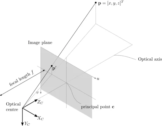
3.3 Projection in the pinhole camera model. . . 21

3.4 Ideal horizontal stereo vision geometry. . . 23

3.5 Epipolar geometry for general stereo camera alignments. . . 23

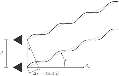
3.6 Angle extraction by the principle of phase monopulse . . . 24

3.7 Manual measurement labelling for extrinsic sensor-to-sensor calibration. . . 26

3.8 Extrinsic calibration results. . . 28

4.1 Diagram of the stereo vision measurement extraction algorithm. . . 29

4.2 DBSCAN reachability illustration. . . 33

4.3 Linear frequency modulation waveform. . . 34

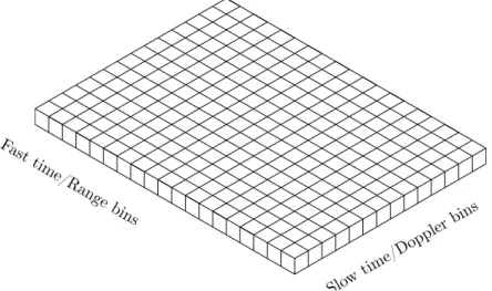
4.4 Two-dimensional slow-time fast-time pulse matrix. . . 35

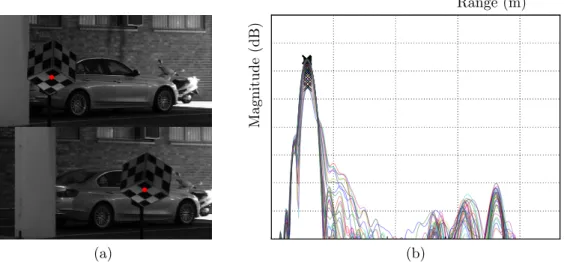
4.5 Illustration of the Complex range-Doppler map. . . 36

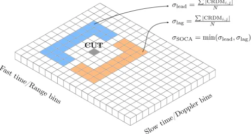
4.6 Calculation of the interference statistic in the smallest-of cell-averaging con-stant false alarm rate algorithm. . . 37

7.1 Flow diagram of the proposed DATMO system. . . 57

7.2 An illustration of the over-segmented clusters extracted by the vision detection algorithm. . . 62

7.3 Visualisation of the track-to-track fusion algorithm. . . 64

7.4 Visualisation of a target’s extent estimate that result from GIW-PHD filtering. 67 8.1 Visualisation of the simulation environment. . . 70

8.2 OSPA simulation results of the GM-PHD filter and the GIW-PHD filter. . . . 73

8.3 Cardinality simulation results of the GM-PHD filter and the GIW-PHD filter. 74 8.4 Diagram of the track-to-track fusion simulation. . . 75

8.5 OSPA simulation results of the track fusion algorithm. . . 76

8.6 Cardinality simulation results of the track fusion algorithm. . . 77 viii

(10)

8.7 OSPA simulation results of the vision-only fusion algorithm. . . 77

8.8 Cardinality simulation results of the single-sensor simulation. . . 78

8.9 Frame from the Helshoogte dataset. . . 80

8.10 OSPA and cardinality evaluation results for the Helshoogte sequence. . . 81

8.11 Frame from the R44 dataset. . . 82

8.12 OSPA and cardinality evaluation results of the R44 sequence. . . 84

8.13 Missed detection in the Merriman sequence. . . 85

(11)

List of Tables

4.1 Radar operating parameters. . . 38

8.1 Tracking performance metrics for the Helshoogte sequence. . . 81

8.2 Tracking performance metrics for the R44 sequence. . . 83

8.3 Tracking performance metrics for the Merriman sequence. . . 86

(12)

Nomenclature

ACC adaptive cruise control

ADAS advanced driver assistance system CFAR constant false alarm rate

CPI coherent processing interval CPU central processing unit CRDM complex range-Doppler map CRF camera reference frame CUT cell under test

DATMO detection and tracking of moving objects

DBSCAN density-based spatial clustering of applications with noise EM electromagnetic

FAST features from accelerated segment test FFT fast Fourier transform

FMCW frequency modulated continuous wave GIW Gaussian inverse Wishart

GIW-PHD Gaussian inverse Wishart probability hypothesis density GM-PHD Gaussian mixture probability hypothesis density

GNN global nearest neighbour IF intermediate frequency IMU inertial measurement unit IQ in-phase quadrature

JPDA joint probabilistic data association KL-diff Kullback-Leibler difference

KL-div Kullback-Leibler divergence LFM linear frequency modulation lidar light detection and ranging MHT multiple hypothesis tracking MOTA multiple object tracking accuracy MOTP multiple object tracking precision MTT multi-target tracking

NN nearest neighbour OBC on-board computer

(13)

Nomenclature xii

OSPA optimal subpattern assignment

P3-AT Pioneer 3-AT

PDA probabilistic data association pdf probability density function PHD probability hypothesis density radar radio detection and ranging RCS radar cross section

RF radio frequency RFS random finite set RMS root-mean-square RRF radar reference frame

SLAM simultaneous localization and mapping

SOCA-CFAR smallest-of cell-averaging constant false alarm rate sonar sound navigation and ranging

SPD symmetric positive definite SSD solid-state drive

UKF unscented Kalman filter WRF world reference frame

(14)

Mathematical Notation

X Matrix

X Random finite set

X Set

x Vector

B(_·) Bhattacharyya distance

N(·) Gaussian distribution

IW(·) Inverse Wishart distribution

W(·) Wishart distribution

p(_·) Belief distribution

f(_·) Dynamic model

h(_·) Measurement model ˆ

(_·) Expected value operator

⊗ Kronecker product

¯

(_·) Mean operator ˜

(·) Scattering matrix operator

h·i Set partition operator

(15)

Chapter

1

Introduction

Environment perception entails the establishment of spatial and temporal relationships relating a robot and its surroundings. Environmental perception is an important require-ment for the autonomous operation of mobile robots and also forms the basis of various advanced driver assistance systems (ADASs). Perception is used for the automation of vehicle navigation, or where potentially dangerous work may be assigned to robots. To navigate reliably, autonomous vehicles should form an understanding of their surrounding scene. In the same manner, driver assistance systems perceive the environment to provide additional safety features to the occupants. Information that result from the perception process serve as input for path planning or collision avoidance algorithms, providing the necessary means for autonomous navigation decision making.

1.1

Overview of Environmental Perception

The perception process is usually divided into two categories, namely: simultaneous local-ization and mapping (SLAM) anddetection and tracking of moving objects (DATMO) [1].

In SLAM, the purpose is to localise the robot with respect to static objects (landmarks) in the environment. The majority of SLAM applications assume a static environment, or scenarios in which static and dynamic objects can be distinguished. SLAM results in a global pose (position and orientation) estimate of the robot as well as a map containing the position of some landmarks. The map is typically sparse, since most SLAM algo-rithms focus only on prominent landmarks. SLAM combines motion information with landmark measurements. Motion information is acquired from ego-motion estimation, which pertains to the process of estimating one’s own movement. Ego-motion-based nav-igation in the absence of SLAM is called dead-reckoning. Pose estimates resulting from dead-reckoning are based solely on motion information, and suffers from severe drift due to error accumulation over time. Dead-reckoning navigation naturally extends to SLAM in many permitting environments where adequate landmarks are available. The primary difference between dead-reckoning and SLAM is that in SLAM, landmark locations are maintained in a global map and used to localise the robot more accurately, whereas the former only integrates motion estimates.

DATMO is the detection and tracking of moving objects. Autonomous vehicles may encounter various moving objects with whom they need to interact in a safe manner. For this to be achieved, position and velocity estimates of every moving object in the robot’s locale have to be calculated. Some ADAS applications, such as adaptive cruise control

(16)

(ACC), require similar information, with the goal of improving the safety of road navi-gation. DATMO is a fundamental requirement for the task of collision avoidance in both autonomous navigation and ADAS, as it allows for the prediction of object trajectories over time.

DATMO and SLAM are mutually beneficial [2,3]. Knowledge of moving objects enable their exclusion in SLAM calculations, thereby increasing pose estimation accuracy. More-over, a precise localisation system is essential for moving object tracking from a moving platform [3]. In conjunction, SLAM and DATMO satisfy both the safety and localisation demands of autonomous navigation [3].

Exteroceptive sensors provide the information required for the task of environmental perception. Radars, cameras and lidars are among the common sensors utilised in this regard. These have different properties regarding accuracy, cost, failure cases and more. Any single sensor, however, is inadequate for robust perception in challenging scenar-ios, prompting the fusion of information from different types of sensors. This practice, known as data fusion, can introduce redundancy, potentially increasing the confidence

and robustness of the perception system as a whole. The application of data fusion is also encouraged by distinct sensor types that exhibit complimentary characteristics.

1.2

Problem Statement

The work in this project relates to the DATMO facet of environmental perception. In particular, the focus is on data fusion of radar and stereo vision as a means to implement a DATMO system. Combining the information from different sensing modalities adds redundancy and increases estimation accuracy. The goal is to develop a radar-vision fusion approach tailored specifically for DATMO in dynamic, ground-based environments. A moving platform of which the ego-motion is assumed available serves as the carrier for the respective sensors. The system should be able to identify, localise and track any non-stationary object that is within the sensors’ field-of-view. Target estimates that are output by the system should be relevant for collision avoidance and autonomous navigation applications.

1.3

Background

The DATMO problem is typically formulated in a Bayesian state estimation framework, involving the chronological steps of data segmentation or measurement extraction, data association and filtering. Methods that proceed in the described manner are categorised as traditional DATMO [4]. Data segmentation aims at the division of sensor data into meaningful pieces such as points, point clusters or line features. This process encompasses the detection part of DATMO, in which the purpose is the identification of moving objects in the environment and the arrangement of the sensor information in a form suitable for subsequent processing.

Multi-target tracking (MTT) follows the measurement extraction process in traditional

DATMO, addressing the data association and filtering steps. In MTT, the objective is to determine the number of dynamic objects and their states based on noisy sensor measure-ments [5]. The data association process entails the assignment of extracted measuremeasure-ments to object tracks; an ambiguous process due to the unknown origin of measurements. Es-tablished MTT algorithms include global nearest neighbour (GNN), joint probabilistic

(17)

CHAPTER 1. INTRODUCTION 3 data association (JPDA) [6] and multiple hypothesis tracking (MHT) [7]. The data as-sociation process is the only way in which the above mentioned algorithms differ, and is also considered as the most complex aspect of MTT [5, 8]. Associated measurements are filtered in what is the final stage of traditional DATMO. Filtering is the estimation of the underlying state of as system. The result is estimates of the state of moving targets in the environment, e.g. position, velocity and shape.

Variations to traditional DATMO include model- and grid-based approaches [4]. Model-based DATMO avoids the difficult problem of data association by incorporating an object model that dictates measurement to target correspondences. In the setting of autonomous navigation, such models usually include a description of the geometric shape of an object. Grid-based frameworks do not track targets at object level, but rather represent the in-formation using cells into which the environment is discretised. A cell’s state is described by a notion of occupancy and velocity. Occupancy grids may be used to implement stand-alone DATMO systems, or to render information that result from traditional DATMO more suitable for path planning and navigation [9].

Achieving reliable performance in real-world environments is a complex challenge in DATMO. Even though the DATMO problem is solved theoretically [3], it cannot shun from hardware inadequacies. Sensors may fail when presented with adverse conditions due to physical limitations or phenomena inherent to their operation. Furthermore, ob-jects may proceed undetected when the available sensors are not suited to detect them. All exteroceptive sensors commonly used in DATMO have undesirable properties. Radar exhibits excellent all-weather operation and is accurate in range, but lacks in its ability to detect targets with low reflectivity. Camera systems provide rich appearance informa-tion, are accurate in angle, but perform poorly in ranging applications and are adversely impacted by poor visibility and lighting conditions. Lidars are accurate in both range and azimuth, but suffer in unfavourable weather conditions.

The described limitations serve as encouragement for data fusion. Fusion practices are aimed at circumventing problems arising from sensor deficiencies by exploiting data redundancy. Generally, multi-sensor data fusion offers significant advantages over the use of a single source [10]. The availability of various observations of a single object provides a statistical advantage. Moreover, increased accuracy can be achieved by considering individual sensor properties during fusion.

An integral part of all multi-sensor data fusion algorithms is estimation [11]. The struc-turing of the estimation process is generally used to distinguish different architectures. Sensory data may be combined at different levels and in a variety of fusion architectures. Techniques for the fusion of raw sensor data typically involve classical detection and es-timation methods [10]. In these cases, the problem is usually cast into a Bayesian state estimation framework adapted for multiple sources. Alternatively, fusion may proceed after local processing at each sensor node, or in hybrid configurations containing elements of both.

1.4

Objectives

This thesis presents a radar and stereo vision data fusion method for DATMO. The project objectives are listed below:

1. The main research objective is the fusion of radar and stereo vision information for DATMO. Data fusion should improve the accuracy and robustness of the system.

(18)

2. Another primary objective is the development of a state estimation framework. The implementation should allow the states of numerous moving objects to be inferred from the sensor measurements.

3. A secondary objective of the research to perform measurement extraction on the respective sensors’ data to detect moving objects. Detection is required in order to enable the demonstration of data fusion and state estimation. Measurement extraction methods should consider generic object classes.

1.5

Project Approach

In this project, information from a short range frequency modulated continuous wave (FMCW) radar and stereo vision cameras are fused for DATMO. Leveraging the angular resolution capabilities of camera sensors may address one of the main shortcomings of radars, while radar range measurements are more accurate compared to that of vision. The detection process is performed for both subsystems individually: a sparse motion-based method identifies moving clusters in image sequences, while radar detection is based on standard Doppler analysis. Separate state estimators are implemented for the respective subsystems. A track-to-track data fusion architecture is developed in which radar and image feature tracks are subsequently combined. Fused estimates serve as measurements in a multi-target tracking framework with explicit provision for extended targets. Figure 1.1 illustrates the processing pipeline of the proposed algorithm.

Data fusion Feature tracking and clustering State estimation Stereo images Radar measurements Extended target tracking

Figure 1.1: Radar-vision data fusion system diagram.

The document is structured as follows. Firstly, a review of relevant research in the fields of DATMO, estimation and data fusion is presented in Chapter 2. Current ap-proaches to combine radar and vision information are also discussed. Chapter 3 describes the physical characteristics that govern measurement generation for radars and stereo vision cameras. The chapter concludes with the presentation of an extrinsic calibration method that is used to determine the relative sensor-to-sensor alignment. Chapters 5 and 6 provide the theoretical foundation for the multi-target tracking framework. The proposed data fusion algorithm is described in Chapter 7. Chapter 8 contains a pre-sentation of relevant results and the analysis thereof. Concluding remarks are given in Chapter 9.

(19)

Chapter

2

Literature Review

This chapter details the techniques common to DATMO and data fusion. The goal is to familiarise the reader with the concepts involved in these fields. A discussion of sensors for object detection, including an examination of measurement extraction techniques, is firstly presented. This addresses the detection aspect of DATMO. State estimation and multi-target tracking is subsequently reviewed. Scene and target modelling, as well as data fusion are coupled to the tracking process, and discussed in the following sections. Finally, the current state of the field of radar and vision information fusion is presented.

2.1

Exteroceptive Sensors for Object Detection

In a DATMO setting, exteroceptive sensors gather information that is required for object localisation by surveying the surrounding environment. The following subsections provide a description of the properties and detection methods for different sensor types.

2.1.1

Radar

Radars operate by transmitting radio frequency (RF) electromagnetic (EM) waves and subsequently analysing signals reflected from surrounding objects. By measuring the time delay and phase shift of received signals, the distance and velocity of a target may be determined. The bearing of detections can be retrieved using directional antennas or phase comparison techniques. Sensors following the aforementioned principle of transmission and reception are labelled as active sensors.

In contrast to other exteroceptive sensors, radar’s RF waves experience minimal at-tenuation when penetrating particles such as fog, dust, rain, foliage and smoke [12]. The attenuation caused by these materials is highly dependant on the centre frequency of the waveform, with greater attenuation at higher frequencies [12]. Detrimental to radar-based object detection is its reliance on radar cross section (RCS). The RCS of a target describes its apparent size from the radar’s perspective [12]. Large RCS fluctuations may be encountered in a ground-based environment, rendering some objects undetectable.

Radar measurements are generally considered accurate in range, but inaccurate in an-gle. The angular resolution in ordinary radar operation is determined by the beamwidth of the receive antenna, which in turn is dependant on the centre frequency and physical antenna size. A narrow beam allows more accurate angular measurements, but is not suited to observe large sections of the environment, i.e. to perform volume searches. To

(20)

observe a large volume requires either a wide beam, or manual or electronic beam steer-ing. Within-beam angular discrimination is possible when several receive antennas are available, using a technique called monopulse. The monopulse mode of operation enables volume search and angular discrimination requirements to be fulfilled simultaneously.

Measurement error may arise due to multipath effects. These errors occur when the wave propagates back to the radar by more than one path. The increase in propagation distance delays the signal, creating the impression of a false target that is at a greater distance [13]. Multipath increases with wavelength, making radar more likely to suffer in comparison with sensors operating in or near the light spectrum [12].

Millimetre wave radar is the preferred candidate in the field of robotics since applica-tions are often subjected to size and mass constraints. This class of radars operate in the range of frequencies between 30GHz and 300GHz. The short wavelength of millimetre wave radars is its primary advantage, allowing the use of physically small antennas [12].

2.1.2

Sonar

The operating principle of sonar is similar to that of radar. Sonar relies on mechani-cal instead of EM waves, thus requiring a physimechani-cal medium for signal propagation. The physics of acoustic sensing is not favourable for environment perception [14], and it there-fore sees limited use in DATMO applications. All solid surfaces are acoustic reflectors, and most surfaces display mirror-like (specular) acoustic behaviour [14]. The consequence of specular scattering is that angled surfaces reflect the incoming signal away from the source, thereby hindering detection [14]. Specular scattering may also introduce multi-path ranging errors [9]. Sonar is best suited to underwater applications, due to reduced attenuation [15] and since other exteroceptive sensors are incapable of operating in water.

2.1.3

Lidar

Lidars are among the most commonly used and versatile sensors for perception appli-cations. Like radar and sonar, lidar measurements are in range-bearing form. Lidars retrieve distance by measuring the time-of-flight of a transmitted light beam [4]. The sensor exhibits excellent angular resolution and accurate range measurements, enabling lidar’s use in high performance perception systems. Two-dimensional lidars return very sparse measurements much like narrow beam radars. Three-dimensional lidars are able to perform volume searches, but they are very expensive.

Backscatter from weather phenomena such as rain, fog, dust or snow may result in unwanted detections [16]. Lighting conditions may also hinder reliable detection, e.g. light absorbing material or the presence of direct sunlight [9]. The vulnerability of lidar to external factors is its most significant deficiency.

2.1.4

Vision

The abundance of cheap camera sensors has contributed to the extensive use of computer vision for environmental perception. Camera systems are versatile, unobtrusive, and the development cycle is easily initiated with inexpensive commercial components. Cameras provide very accurate angular measurements and, for stereo configurations, coarse range. Semantic information may also be extracted in addition to distance and angle. The influence of external environmental factors on vision systems are generally the same as for lidars.

(21)

CHAPTER 2. LITERATURE REVIEW 7 The wealth of information provided by cameras allow for a multitude of different approaches to obstacle detection, permitting a more detailed discussion. The following sections detail the most prominent vision-based moving object detection methods. For the purpose of this discussion, the termsobject detection and segmentation will be used

interchangeably.

Background Subtraction

Background subtraction is perhaps one of the simplest and most intuitive methods of motion segmentation in images. It amounts to pixel-wise subtraction of a background model from the current frame, thereby emphasizing areas where the image has changed. Background subtraction assumes a stationary camera and is therefore not suitable for use on a moving platform.

Attempts have been made to perform background subtraction for moving cameras [17, 18]. In these methods motion induced by camera movement has to be corrected for. This relies on accurate estimations of ego-motion which is attainable through the use of an inertial measurement unit (IMU). Ego-motion may also be estimated by using optical or range sensors.

Geometric Measurements

Certain assumptions allow general physical attributes to be used for the detection of generic object classes. Examples include texture, edges, shadows and symmetry infor-mation. It is reasonable to expect that arbitrary objects will contain some combination of geometric features, although some are more restrictive than others; for example sym-metry. A downside of this approach is that stationary clutter and targets of interest are indistinguishable. Researchers therefore usually limit the implementation to areas where motion is assumed [19, p. 346]. In an ADAS environment for instance, the road surface would first be detected, and the result used to only consider geometric shapes that are above the road surface.

Optical Flow

An important cue in image analysis is the relative movement of visible surfaces between successive frames. Two-dimensional image plane motion fields, or optical flow, provide important information regarding the spatial arrangement of a scene. Various techniques exist for computing optical flow, including differential-, energy-, correlation- and feature-based [20]. Optical flow may be computed for either the entire image (dense) or for selected patches only (sparse). The addition of range data to optical flow calculations result in three-dimensional motion fields called scene flow.

Differential optical flow is the most widely used technique, and is based on the as-sumption that the intensity of a moving pixel remains constant over time, i.e.

I(u, v, t) =I(u+ ∆u, v+ ∆v, t+ 1) (2.1) where [∆u,∆v]T _{is the flow vector of pixel} _[_{u, v}_]T _{from time} _t _to _t_{+ 1} _{[21]. The flow}

vector may be solved by optimizing the Taylor series expansion of Equation (2.1), often by means of the Lucas-Kanade method [22].

Differential optical flow can be categorised into local and global methods according to the type of energy function they optimise. Local optical flow methods are relatively

(22)

robust under noise, but do not result in motion estimates at every pixel [21]. Smoothing constraints allow dense motion fields, and are usually formulated in terms of a global optimisation problem containing local (data) and smoothing terms. Textureless regions is problematic for both local and global optical flow calculations [23]. Local methods generally disregard such regions, while the smoothing constraints in global methods enable their resolution.

Discontinuities in the motion field can assist in the segmentation of an image into regions that correspond to different objects. Various authors have used this principle for generic moving object detection in image sequences [24–26]. Klappstein et al. [24] demonstrates this principle using both monocular and stereo vision. By introducing motion constraints, features in the image are either considered as static or belonging to moving objects. Features are then clustered into coherent objects and subsequently used as seeds for segmentation using graph cuts. A similar approach is followed by Wedel et al. [25] using dense scene flow.

Appearance-Based Methods

Appearance-based methods involve the implementation of machine learning techniques to learn semantic patterns in images. A common approach is supervised learning, which entails the training of a classifier using manually labelled data. A drawback of these methods is that classifiers are class specific. Multiple object detection would require as many classifiers, which is often impractical due to the computational burden. Learning methods do not require ego-motion estimates and are robust against irregular movement of the sensing platform.

The following paragraph motivates the choice of radar and vision for data fusion. As was stated earlier, the performance of sonar is not up to standard in air. Lidars take accurate measurements, but an expensive 3-D lidar is required for volume searches. Vision, and more recently also radar, are the affordable options for data fusion applications. Both are able to do volume searches, and their complimentary characteristics favour data fusion. Moreover, radar-vision fusion may be extended to small airborne platforms since both sensors are lightweight.

2.2

Recursive Bayesian State Estimation

The eventual purpose in DATMO is to extract the states of moving object using the information from exteroceptive sensors. The standard approach in which these quantities are obtained relies on stochastic modelling of the processes surrounding target dynamics and measurement generation. The Bayes filter provides a rigorous theoretical foundation to infer target states using the above mentioned probabilistic models.

In a Bayesian context, the desired target states are represented as a probability dis-tribution p(_·), also know as the belief. The task is to estimate, at each time step, the

current states of a target given all sensor measurements that have been collected, i.e. the

posterior distribution p(xk|z1:k), where xk is the state vector at time k, and z1:k is all

target measurements up to and including timek.

The Markov assumption allows the elegant recursive formulation of state estimation, i.e. the Bayes filter. In a Markov process, the dynamic model is assumed to be independent

(23)

CHAPTER 2. LITERATURE REVIEW 9 of all previous states given the present state, i.e.

f(xk|x1:k−1) = f(xk|xk−1). (2.2) The Bayes filter consists of two steps, namely prediction and correction. Prediction describes the transition of the belief distribution from the previous time step to the current without additional observations of the target. Evaluating the prediction step results in theprior distribution, and requires a model of the target’s dynamic behaviour. Formally,

the prior is given by [9, p. 27]

p(xk|z1:k−1) =

Z

f(xk|xk−1)p(xk−1|z1:k−1)dxk−1, (2.3) where f(xk|xk−1) is a probability distribution modelling the target dynamics. Sensor information is incorporated in the correction, or measurement update, step. The required posterior can be calculated according to Bayes’ rule as

p(x_k_|z1:k) =

h(zk|xk)p(xk|z1:k−1)

R

h(zk|xk)p(xk|z1:k−1)dxk

, (2.4)

where h(z_k_|x_k) is the sensor or measurement model, which is a conditional distribution modelling the measurement generation. The denominator of Equation (2.4) is simply a constant and can be considered a normalisation factor.

Equations (2.3) and (2.4) define the single-source, single-target Bayes filter, which forms the theoretical foundation for single-target tracking, single-target information fu-sion, as well as multi-sensor and multi-target detection, tracking and data fusion [27].

2.3

Multi-Target Tracking

En route to implementing a practical target state estimator, one of the fundamental as-sumptions of the Bayes filter needs to be addressed, namely perfect measurement-to-track associations (hence the term ‘single-source, single-target’). The environments under con-sideration for DATMO fail to comply with this assumption. A typical MTT scenario is shown in Figure 2.1. The expected observations at timek,h(ˆx(_ki_|)_k₋₁), are drawn along with their validation gates. The state vectorx(_ki_|)_k₋₁ describes the track of theith _{target. A gate} defines the region where measurements will be considered for association to the particular target track, and is a concept utilised in many multi-target tracking (MTT) algorithms. The presence of multiple targets and clutter entail uncertain relationships between mea-surements and sources: an individual measurement may have originated from any one of the targets or from static clutter in the environment. Each incoming sensor report needs to be assigned to the correct target track to facilitate robust estimation. Ambiguous data association is the primary motivation for MTT techniques. The remainder of this section will present some established and more recent methods that address data association, which is the defining component of different MTT algorithms.

2.3.1

Global Nearest Neighbour

The simplest and most intuitive data association method is the nearest neighbour (NN) algorithm. NN assigns the measurement closest in statistical distance to the predicted track to be used in the measurement update. The NN algorithm is in fact a single-target

(24)

h(ˆx(1)_k_|_k₋₁) h(ˆx(2)_k_|_k₋₁) h(ˆx(3)_k_|_k₋₁) z(3)_k z(2)_k z(1)_k z(4)_k z(5)_k

Figure 2.1: Target validation gates in a typical multi-target tracking scenario. A gate is centred on the expected observation position h(ˆx(_ki_|)_k₋₁), and is proportional to the innovation distribution. Measurements that fall within a target’s gate are considered for subsequent data association.

data association method, since surrounding targets and their associations are not taken into regard when searching for the nearest measurement. Its extension to multiple targets is knows as global nearest neighbour (GNN).

GNN makes a hard assignment of at most one observation to a track when measure-ments arrive at any given scan time [5]. In contrast to single-target nearest neighbour data association which is only locally optimal, in GNN, distances between all measurements and tracks are considered when calculating the association assignments. The eventual as-signment mapping is chosen as the most likely solution among all mappings [28]. Clutter measurements or new targets account for unassociated measurements, which proceed to initiation logic in order to form new target tracks.

2.3.2

Joint Probabilistic Data Association

Fortmann and Bar-Shalom [29] introduced the joint probabilistic data association (JPDA) filter, which is the multi-target extension of single-target probabilistic data association (PDA) filter. Both standard PDA and JPDA are non-optimal in the sense that they require Gaussian approximations of the posterior distributions [30]. In PDA, all mea-surements that are within the target’s validation gate are considered in the measurement update step. This is implemented by substituting the traditional single-measurement innovation with a weighted combination calculated from all gated measurements. The weighting factors are calculated in accordance with the likelihood of the particular mea-surement. Such probabilistic measurement-to-track associations of numerous observations are known as soft assignments. Soft association techniques are slightly more complex than their hard assigning counterparts, but they prove much more effective in cluttered envi-ronments.

The key difference in multi-target JPDA, as opposed to single-target PDA, is the way in which the mixture weights are calculated [28]. The individual measurement likelihoods used in determining the weights are computed with all the targets and measurements in

(25)

Figure 2.2: Progression of the multiple hypothesis tracking algorithm. At each time step, a hypothesis is created for all measurements that fall within the validation region of a target. An additional hypothesis to account for missed detections is also initialised. Grey lines indicate either a prediction or measurement update step. The enlarged blue ellipse is used to show the second update recursion for the particular target. Figure adapted from Durrant-Whyte [31].

consideration. The process can be quite complex and is also dependant on an assumed clutter distribution. Upon calculating the weights, the JPDA algorithm proceeds in the same manner as the PDA filter [31].

2.3.3

Multiple Hypothesis Tracking

The preceding data association approaches consider target states of a single time step in their calculations. All previous information is encapsulated in the probability distributions of the respective targets. The multiple hypothesis tracking (MHT) algorithm introduced by Reid [7] specifies a framework that regards target states across multiple scan times. The MHT filter initialises separate tracks, or hypotheses, for every measurement in a target’s validation gate. In addition, a hypothesis is also generated to represent the missed detection/false alarm case. The indiscriminate associations result in a ‘tree’ of hypotheses being spawned for a target at every time step. The likelihood of a particular branch of the tree is given by the recursively evaluation of the association likelihoods along the branch. To limit the combinatorial growth in track hypotheses, a pruning strategy based on the likelihoods is usually implemented [31]. The partial tree structure and hypothesis generation of a single target over two time steps is shown in Figure 2.2.

The MHT algorithm described above and illustrated in Figure 2.2 is known as track-oriented MHT, which is one of the most advanced MTT methods [5]. MHT is generally the

(26)

apt choice in situations with high track uncertainty, e.g. crossing or manoeuvring targets, and is also effective in clutter [5, 31]. Practical implementation of the method requires careful consideration with regards to pruning in order to limit memory consumption.

2.3.4

Probability Hypothesis Density Filter

Mahler’s [32] random finite set (RFS) modelling permits the proper Bayesian formulation of multi-target recursive filtering. In this scheme, both target states and observations are modelled as random sets consisting of a random number of random elements. RFS modelling stems from the intuitive finite set form of representation for a collection of targets and measurements, i.e.

Xk = n x(_ki)oNtargets,k i=1 , (2.5) Zk = n z(_ki)oNmeasurements,k i=1 , (2.6)

where the elements ofXk represent individual target state vectors, and those of Zk

indi-vidual observation vectors. In this setting, uncertainty in target states is characterised by modelling the state and observation finite sets as random finite sets, in analogy to the random vector modelling in single-target systems.

The theoretical development lead to the multi-target equivalent of the single-target Bayes filter. As is the case for the single-target variant, the resulting recursive equations are intractable. Approximations involving the propagation of lower order statistical mo-ments have been implemented by Mahler [32] and Vo [33]. These lower order momo-ments are termed probability hypothesis densities, and the resulting recursive filter the probability hypothesis density (PHD) filter.

The key advantage of RFS-based recursive filtering is the avoidance of the data asso-ciation problem. The algorithm does not implement any form of measurement-to-track assignments, due to the set-based target and observation modelling. In the PHD filter, explicit track formation is avoided and exchanged for a representation that describes the probability of a target being present in a certain space [5]. Consequently, target identity tracking is not incorporated in the standard PHD algorithm.

2.4

Measurement Modelling

The discussion in Section 2.2 detailed the underlying theory upon which target tracking is built. As was mentioned, the Bayes filter recursion requires dynamic and measurement models for the posterior states to be inferred. This section will discuss common modelling methods with regards to the measurement model. These models describe the distribution of sensor measurements conditioned on the target state.

The standard sensor model used in multi-target tracking algorithms assume negligible object extent by modelling a target as a point in space [34]. The premise of a DATMO or ADAS application entails that objects appear ‘near’ the sensing platform. As a con-sequence, an object will most often occupy multiple sensor resolution cells and generate numerous measurements per time step, thereby violating the point target assumption. Tracking these objects give rise to the problem of extended target tracking. Formally,

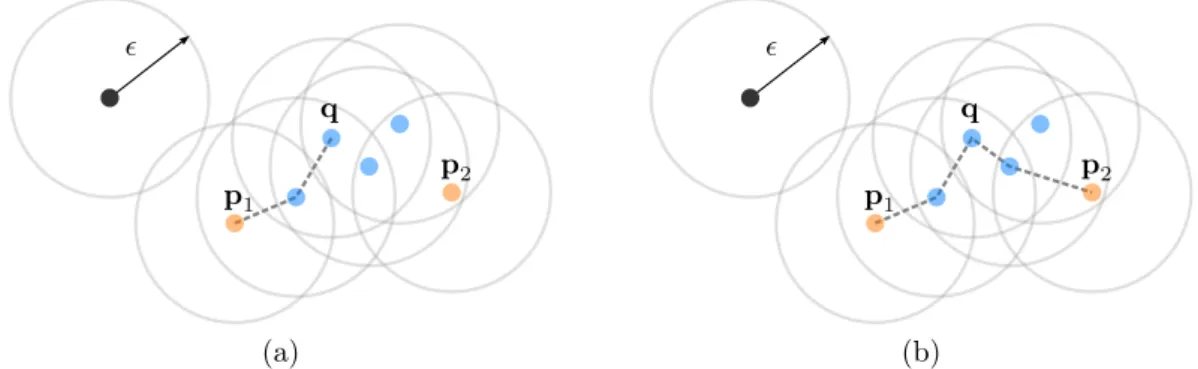
an extended object is defined as one which may generate a varying number of spatially distributed measurements per scan [34]. An illustration of an extended target is given in

(27)

CHAPTER 2. LITERATURE REVIEW 13 Figure 2.3. Object shape, as well as the expected number of measurements per object can be incorporated in extended target models.

Related but distinct to extended target tracking is the problem of group tracking. Group targets consist of a number of a objects that move in a coordinated and interacting fashion [35]. Extended target tracking techniques are often directly applicable to group tracking due to the similarities that distinguish these problems from conventional point object tracking. A notable difference is the interacting nature of groups that is not present in extended targets. The discussion will proceed with emphasis on extended targets because of their prevalence in DATMO and ADAS applications.

Extended target models usually assume a specific geometric shape. The parameters that describe such a shape are appended to the target state vector and inferred from observations. For this to be achieved in the Bayesian filtering paradigm requires the specification of an augmented sensor model that explicitly accounts for the target extent. Common geometric models include curves in 2D or 3D space, ellipses or rectangles.

2.4.1

Spatial Distribution Models

Gilholm and Salmond [36] developed the proper Bayesian formulation for extended target tracking, in which the target is represented by a spatial probability distribution. In addition to the spatial distribution, the number of measurements originating from a target is modelled as a Poisson process [36]. The spatial model represents the distribution of measurement sources across the target, and may take the form of general shape models such as lines or circles. Measurements are assumed to be independent realisations from the spatial probability model convolved with a sensor error model [36]. Therefore, the probability density function (pdf) of a single target measurement, as described by the spatial model, is given by

h(z_|x) =

Z

p(z_|y)p(y_|x)dy, (2.7)

wherep(y_|x)denotes distribution of measurement sources conditioned on the target state

x, and p(z_|y) denotes the distribution of an individual measurement z conditioned on the measurement generating sourcesy. The eventual likelihood is a combination of Equa-tion (2.7) and the Poisson distribuEqua-tion that models the expected number of measurements. The inclusion of a geometric model leads to a significantly more complicated sensor model

Figure 2.3: Illustration of an extended target. An extended target occupies multiple sensor resolution cells and may as a result generate numerous spatially distributed measurements per scan.

(28)

compared to the point target case. As a result, the implementation is usually restricted to particle filters [36].

2.4.2

Random Hypersurfaces

An extended target algorithm based on the concept of a random hypersurface was intro-duced by Baum and Hanebeck [37]. Any individual measurement is modelled as a noisy observation of a measurement source on the target surface [37]. A measurement source is assumed to be a randomly generated hypersurface representing a scaled version of the target shape. A two step process therefore defines the generation of measurements: first, a measurement source model is generated, after which the sensor error model describes the observations to be expected from the particular source. The likelihood of an individual measurement is determined by evaluating the combined probability of the measurement source given the current shape parameters, and the measurement given the source. Vari-ous shapes can be used with random hypersurface models, including ellipses and arbitrary star-convex1 _{patterns [37,38].}

The random hypersurface algorithm does not explicitly model the position of mea-surement generating sources, but rather estimates the shape of the target [38]. Explicit source models are common in extended target tracking. However, they require proper models of the measurement generating sources and sensor resolution that is high enough for the different sources to be resolved [38]. In addition, explicit source models may suffer when sensor returns are influenced by the target’s orientation to the sensor.

2.4.3

Random Matrices

Koch [39] formulated a very efficient model for extended target tracking based on the use of symmetric positive definite (SPD) random matrices. Each measurement is interpreted as a measurement of the object’s centroid with an error that is proportional to the ob-ject’s extent [39]. By this procedure, the extent is incorporated into the measurement likelihood function as a covariance substitution, allowing very simple update equations. SPD matrix representation implies an elliptical object shape, and is modelled using an inverse Wishart distribution. The inverse Wishart distribution is the conjugate prior for the unknown covariance matrix representing the measurement spread [34,39]. The novelty of the method, in contrast to previous elliptical shape modelling, is the joint estimation of centroid kinematics and physical extent in a rigorous Bayesian framework [40]. A short-coming of Koch’s original method is the neglect of any statistical sensor error. Feldmann et al. developed an adapted random matrix algorithm that takes both the object extent and sensor error into account when modelling the spread of measurements [41]. The for-mulation is similar to Koch’s, and the shape representation is exactly the same. Without the inclusion of the sensor error, the algorithm would effectively estimate object extent plus sensor error.

In both random matrix approaches, the extent is updated by a weighted combination of matrices representing the predicted extent, measurement scattering and the mean mea-surement deviation respectively [39, 41]. The meamea-surement update formulas derived for the random matrix algorithm are considerably simpler than those resulting from spatial distribution or random hypersurface modelling, and may be implemented in a linear filter. A limitation of the random matrix model is the elliptical shape constraint.

1_{A set}_S

⊂RN is star-convex with centermif each line segment frommto any point inS is contained inS [38].

(29)

CHAPTER 2. LITERATURE REVIEW 15

2.4.4

Alternative Modelling Approaches

The three extended target tracking algorithms described above make up the current state of the field in Bayesian extended target tracking. Some methods also proceed in a non-Bayesian fashion due to the difficulty of formulating tractable measurement models for extended targets. This is especially common in computer vision applications, where ‘ex-tended’ objects are often tracked using appearance information to match shape kernels between frames [42]. Such approaches are fundamentally different to Bayesian extended target methods, in which shape is inferred over multiple time steps.

The preceding extended target tracking techniques all rely on a state vector repre-sentation for individual targets, in accordance with traditional or model-based DATMO. Grid-based alternatives may also be used to represent the environment. Rather than stor-ing movstor-ing object information in separate state vectors, grid methods rely on a division of the environment into discrete cells. Typical properties that describe each cell, such as velocity and/or occupancy, are subsequently estimated from sensor measurements. In the context of advanced driver assistance system (ADAS), a local grid is typically used to represent the area in front of the vehicle [4, 43]. The grid then serves the purpose of modelling potential dangers rather than building and maintaining a global map [4].

2.5

Data Fusion

The previous sections introduced some of the important concepts relating to Bayesian state estimation and target tracking. The discussion now moves on to data fusion, which has the potential to improve the confidence and robustness of tracking systems.

Multi-sensor data fusion seeks to achieve superior inferences by combining informa-tion from multiple sources [30]. Safety critical systems need to be robust with respect to adverse environmental conditions, and can therefore not dependant on single-source infor-mation. Complimenting characteristics of different sensor types may improve the overall observability of physical target attributes. Multiple reports from comparable sources also improves estimation performance, and is analogous to multiple observations from a single sensor [30, p. 2]. This section introduces the core methods and concepts applicable to data fusion in a DATMO application.

2.5.1

Probabilistic Data Fusion

Optimal fusion in the Bayesian sense relies on the processing of multi-sensor information at a centralised state estimator [5]. Data fusion is then formulated in the classical Bayesian methodology adapted for multiple sources. Consider the synchronous set of observations fromNs,k sensors at scan time k

Zk= n

z(_ki)

oNs,k

i=1 . (2.8)

It is desired to use all the available information to construct the posteriorp(xk|Zk). Direct

implementation of Bayes rule results in

p(xk|Z1:k) =

h(Zk|xk)p(xk|Z1:k−1)

R

h(Zk|x)p(x|Z1:k−1)dx

, (2.9)

which is the multi-sensor equavalent of Equation (2.4). Due to the difficulty in construct-ing the joint sensor modelh(Zk|xk), it is usually assumed that respective sensors generate

(30)

readings independently from one another given the state x, i.e. [31] h(Zk|xk) = h z(1)_k , . . . ,z(Ns,k) k |xk = Ns,k Y i=1 h(z(_ki)_|x_k). (2.10)

Equations (2.9) and (2.10) provide the theoretical grounds for optimal Bayesian multi-sensor data fusion. This formulation of data fusion entails the derivation of appropriate sensor models and application of the above equations in a recursive state estimator. Sen-sor reports are, however, seldom synchronous in real-world scenarios. Fusion may then be conducted by means of separate updates for the respective sensors [44]. Bayesian multi-sensor data fusion is directly applicable to traditional state space models as well as probabilistic grids [11].

2.5.2

Feature-Level Fusion

Bayesian data fusion is not possible in the event that sensors do not measure the same physical phenomena [30]. Sensors are therefore required to report comparable information if the multi-sensor Bayes filter is to be applied. Feature-level fusion entails the extraction of representative features from the sensor data in order to obtain compatible information from numerous sources that may be dissimilar. Pattern recognition techniques such as regression or clustering algorithms can subsequently be implemented on a multi-source feature vector for improved classification or decision making [30].

Both the feature-level and Bayesian techniques are categorised as centralised fusion,

since these methods require low-level sensor data at the fusion centre. Centralised fusion architectures demand high communication bandwidth between individual subsystems and the central processing unit, but is generally considered superior to alternative fusion methodologies.

2.5.3

Track-to-Track Fusion

The previous data fusion techniques require low-level sensor information. Low commu-nication bandwidth or restrictions of legacy sensors may render such data unavailable. Generally, the only available information in these scenarios is the distribution parameters describing target tracks, and combining the information amounts to track-to-track fusion. In classical track fusion, each sensor generates tracks independently from other sensing nodes, before transmitting the pre-processed information to a central processor [30]. Here, tracks are associated and their information combined to acquire more accurate target in-formation.

Data fusion strategies cannot be inhibited to a select number of algorithms, since they can be devised in countless ways. Hybrid configurations between centralised and track-to-track fusion architectures may be implemented, where a combination of pre-processed and raw data is used [30]. Other architectures include distributed fusion, in which sensor nodes are interconnected without the concept of a central processor. However, for the purpose of exteroceptive sensor fusion for DATMO applications, lower level fusion architectures are most applicable.

(31)

CHAPTER 2. LITERATURE REVIEW 17

2.6

Radar-Vision Data Fusion

The foregoing sections laid the groundwork for the analysis of current approaches in radar-vision data fusion. Radar and camera sensors exhibit complimentary sensing char-acteristics that may prove beneficial to combine for DATMO and other environmental sensing purposes. Leveraging the angular resolution capabilities of camera sensors may address one of the main shortcomings of radars, while radar range measurements are more accurate compared to that of vision. The error bounds of these respective sensors are shown in Figure 2.4. The aim is to reduce the estimation error to fit the best of both sensors by proper combination of their information. What follows is an exposition of the state of the field with regards to radar and vision data fusion for DATMO.

Radar error distribution Vision error distribution

Figure 2.4: Vision and radar error characteristics.

2.6.1

Attention Windows

The concept of attention windows is encountered quite often in literature regarding radar-vision fusion [45–48]. In these methods, the radar provides a list of targets which are subsequently processed using image data to refine, validate or classify the target. Radar detections therefore serve as a guide to subsequent image processing algorithms.

Gern et al. [45] demonstrates such an approach to improve the lateral information of an object. Different vision-based operators are defined that vote individually for the centre of a radar attention window. A decision module eventually determines the extent of the object using the output of the operators. Wang et al. [46] follows a similar approach, but instead uses edge and shadow information for determining object extent. An alternative involving machine learning is presented by Ji and Prokhorov [47]. Their approach forwards attention window information to an in-place learning framework to classify objects. The radar effectively reduces the search space of the classification framework, allowing real-time performance.

2.6.2

Fusing Independent Observations

Work where independent observations from the radar and vision subsystems are fused are few in number. Wu et al. [49] demonstrates a feature-level fusion algorithm which

(32)

constructs refined object contours using information from a radar and stereo vision cam-eras. Measurement extraction is initially performed independently for the separate sub-system: the radar tracks point targets, while two-dimensional contours are extracted from the stereo depth maps. Subsequent feature-level fusion involves the association of radar tracks to image contours, and their eventual refinement to obtain improved range and azimuth estimates. Fused contours are ultimately tracked in an extended target tracking framework [49]. Their extended target model does not adhere to proper Bayesian princi-ples, namely joint kinematic-extent estimation, but rather tracks the contour parameters independently.

A solution that borrows from the attention window methodology is presented by Fang et al. [50]. Their algorithm starts by calculating edge maps from stereo image pairs. Edge pixels are subsequently arranged into histogram bins according to their disparity values. Peaks in the resulting histogram serve as hint that an object may be present, and is used to define disparity ranges for subsequent object segmentation. This allows the implementation of a multi-level segmentation procedure based on different disparity intervals. Information describing the number of targets and their distances is optionally incorporated in the specification of depth ranges for vision-based segmentation [50]. Radar detections then essentially guide the multi-level object segmentation.

Richter et al. [51] developed an environmental sensing system that detects both station-ary and moving objects, using ego-motion data along with information from a monocular camera and a radar. The detection process is again executed individually for the sub-systems. In this case, vision-based detection relies on u-shape template matching. These detections are used to verify radar observations and to estimate additional target proper-ties such as width and lateral position [51].

Relatively few sources address the problem of combining the information of radars and cameras. Related work tends more towards lidar-vision fusion due to the rich and con-sistent information extracted by lidars. A common trend among radar-vision fusion liter-ature in short-range applications is the rarity of mathematical techniques such as multi-sensor Bayesian filtering. The apparent reason is the fairly high dissimilarity of the infor-mation provided by these sensors when applied in ground-based DATMO environments, leading researchers to adopt either feature- or track-based data fusion methods.

A notable shortcoming in all the prominent radar-vision fusion sources referenced above is the lack of probabilistic modelling of object extent. The majority of these research efforts focus on radar-guided image processing [45–48,50], feature-based fusion [49] or cross validation of detections [51,52]. Although geometric information is often estimated [49,51], kinematic and extent estimation does not follow the principles laid out in Section 2.4, but rather regards the two as decoupled entities. In addition, multi-target tracking is generally given little attention [45–47].

The work in this project seeks to address the above mentioned shortcomings. Explicit extent modelling and the incorporation thereof in joint kinematic-extent tracking is ex-pected to improve estimation accuracy. Embedding extended target models in advanced MTT algorithms should also contribute to an increase in perception performance.

(33)

Chapter

3

Sensor Configuration

This chapter sets out to describe the hardware involved in the project. Specific sensors have been acquired for the implementation of the proposed DATMO system, and knowl-edge of their operation will aid the subsequent understanding of some hardware specific solutions implemented in the project. To begin, an overview of the components that con-stitute the system will be presented. A thorough discussion with regard to the physical operation of the respective sensors will follow. Finally, the calibration method developed for geometric alignment of the radar and vision subsystems will be presented.

3.1

Hardware Overview

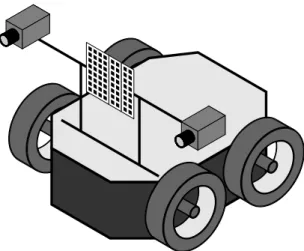
This project’s sensing hardware consists of two Point Grey Flea3 cameras and a short-range radar. The sensors are connected to the on-board computer (OBC) of a Pioneer 3-AT (P3-3-AT) mobile robot to which they are rigidly mounted as shown in Figure 3.1. The P3-AT’s OBC has a dual core processor and runs64-bit Ubuntu Linux. For the purpose of this research, the robot platform was used to gather datasets for offline processing. A solid-state drive (SSD) accompanies the processor to facilitate real-time data storage.

The radar utilised in this work is an Infineon BGT24MTR12 development kit unit, with a centre frequency of24GHz. The radar has one transmit- and two receive patch antennas as illustrated by the checkerboard-like patterns in Figure 3.1. Dual receive antennas allow angular discrimination in one spatial dimension by the principle of monopulse (see

Figure 3.1: Sketch of the sensing platform used in this project. 19

(34)

Section 3.2.3). The radar is operated according to FMCW principles and at a bandwidth of 155MHz. Analog signals from the respective receive antennas’ in-phase quadrature (IQ) receivers are synchronously sampled to render complex-valued information.

The cameras are mounted in a horizontal stereo configuration on either side of the radar as shown in Figure 3.1. The stereo baseline is approximately55cm, which is nearly the same as that of the renowned KITTI dataset [53]. A hardware trigger ensures time syn-chronisation between the respective cameras. Synchronous triggering and global shutters allow precise stereo image pairs to be captured. The cameras are operated in monochrome mode, at a resolution of 1280_×960 pixels. Camera recording is set at 10Hz, while the radar achieves a marginally faster rate.

Both subsystems stream unprocessed data to the OBC. For the radar, this data is in the form of sampled data representing the complex valued signals of the two receive channels. Images are transmitted as 8-bit RAW format. A global CPU timer assigns a time-stamp to every measurement upon its arrival.

Before advancing, a mention of the relevant coordinate systems is in order. With reference to Figure 3.2, three reference frames can be defined. The common frame of reference in which estimation will be performed is the world reference frame (WRF), denoted by W.

A separate frame for the robot is not chosen. Instead, the robot’s position is assumed to coincide with the centre of the camera reference frame (CRF) C. The radar reference

frame (RRF) is denoted by an R. The chosen axes orientations coincides with the usual

stereo vision coordinate frame, with theZ axis pointing out of the camera. The relative

alignment between the RRF and CRF is the subject of Section 3.3.

YW XW ZW YC XC ZC YR XR ZR

Figure 3.2: Coordinate system c