Learning Linear Transformations between Counting-based
and Prediction-based Word Embeddings
Danushka Bollegala1,4,*, Kohei Hayashi2,4, Ken-ichi Kawarabayashi3,4,
1Department of Computer Science, University of Liverpool, Liverpool, United
Kingdom.
2National Institute of Advanced Industrial Science and Technology, Tokyo, Japan.
3National Institute of Informatics, Tokyo, Japan.
4Kawarabayashi ERATO Large Graph Project, Tokyo, Japan.
*Corresponding author
E-mail: [email protected](DB)
Abstract
Despite the growing interest in prediction-based word embedding learning methods, it 1
remains unclear as to how the vector spaces learnt by theprediction-based methods 2
differ from that of thecounting-based methods, or whether one can be transformed into 3
the other. To study the relationship between counting-based and prediction-based 4
embeddings, we propose a method for learning a linear transformation between two 5
given sets of word embeddings. Our proposal contributes to the word embedding 6
learning research in three ways: (a) we propose an efficient method to learn a linear 7
transformation between two sets of word embeddings, (b) using the transformation 8
learnt in (a), we empirically show that it is possible to predict distributed word 9
embeddings for novel unseen words, and (c) empirically it is possible to linearly 10
transform counting-based embeddings to prediction-based embeddings, for frequent 11
words, different POS categories, and varying degrees of ambiguities. 12
1
Introduction
13Representing the meaning of a word is a fundamental task in Natural Language 14
Processing (NLP). Two main approaches for computing word embeddings can be 15
identified in the literature: counting-based approaches, andprediction-based 16
approaches [1]. 17
Counting-based methods represent a target word by the words that co-occur with 18
that target word in various contexts using some co-occurrence measure [2]. Following 19
the distributional hypothesis that states the meaning of a word can be represented using 20
the words that co-occur with that word in different contexts, for example, the words 21
that co-occur with the wordcat such aspet food,dog,cute etc. can be used to represent 22
the meaning ofcat. Various association measures such as the pointwise mutual 23
information (PMI),χ2 measure, log likelihood ratio (LLR) have been proposed in the
24
literature for measuring the strength of the co-occurres between two words. Any word 25
in the vocabulary (i.e. the set consisting of all words in a language) can appear in a 26
co-occurring context. Consequently, under counting-based approaches, a word is 27
represented in a high dimensional (in practice dimensionality greater than 105 are 28
of words will be co-occurring with any given word. Therefore, counting-based 30
embeddings tend to be highly sparse. This becomes problematic when applying 31
counting-based word embeddings as features for representing words in downstream NLP 32
applications such as similarity measurement, or sentiment classification because of 33
feature sparseness. To overcome these disfluencies associated with counting-based word 34
embeddings dimensionality reduction methods such as Singular Value Decomposition 35
(SVD) are often used as a post-processing step. 36
Prediction-based word embedding learning methods [3–5] on the other hand update 37
fixed dimensional word vectors (possibly randomly initialized) such that we can 38
accurately predict the words that appear in a target word in a given context. 39
Prediction-based methods have reported impressive performances across a wide range of 40
NLP tasks such as sentiment classification [6], named entity recognition [7], semantic 41
role labeling [8], and machine translation [9]. Prediction-based word embedding learning 42
methods produce lower dimensional (ca. 100−1000 dimensions are common) and dense 43
word representations. The vector spaces spanned by the prediction-based embeddings 44
are known to demonstrate a certain level of linear structure where subtraction of word 45
embeddings result in vectors that represent the semantic relationships between two 46
words. For example, embedding produced by v(king)−v(man) +v(woman) is shown to 47
be similar tov(queen), where we use the notationv(x) to denote the embedding of the 48
wordx. Unfortunately, the lower-dimensional dense embeddings produced by the 49
prediction-based methods are difficult to interpret compared to the high-dimensional 50
and sparse representations produced by the counting-based methods where each 51
dimension can be explicitly identified with a context word. 52
Despite the success stories of prediction-based embeddings, we understand very little 53
about how they differ from their counting-based counterparts. Levy et al. [10] 54
empirically showed that the differences between the two types of embeddings can be 55
mainly attributable to the differences in hyperparameter settings and pre-processing 56
steps. Intuitively, given that both types of embeddings are learnt from the same source 57
of data, we would expect some relationship between prediction-based and 58
counting-based embeddings. More specifically, because of the high-dimensionality of the 59
counting-based embeddings, they could potentially preserve the information captured by 60
the prediction-based embeddings. 61
But how can we investigate the relationship between these two types of embeddings? 62
Because the two types of embeddings have different dimensionalities, a direct 63
comparison is impossible. However, if the counting-based methods truly capture the 64
same information as the prediction-based methods, then we must be able to recover 65
prediction-based embeddings from the counting-based embeddings. In other words, 66
there must exist aprojection from the high-dimensional, counting-based 67
word-embedding space to the low-dimensional, prediction-based word-embedding space. 68
In this paper, we investigate such a projection with the simplest possible 69
setting—linearity. We propose a method that learns the optimal linear transformation 70
between two given sets of embeddings in a supervised way (i.e., the error between the 71
target and the transformed embeddings is minimized). Because of the cheap 72
computational cost, the linearity assumption allows us to compare a large number (ca. 73
400k) of word embeddings to obtain statistically reliable results. Moreover, if word 74
embeddings can be converted using linear projections, then it provides empirical 75
evidence to the fact that the vector spaces learnt by the prediction-based word 76
embedding learning methods are linear in structure. 77
Our experiments bring a few surprising results (Sections 4.1 and 4.2). First, when a 78
transformation is sufficiently optimized in terms of the training error, the projected 79
embeddings achieve the same performance as the prediction-based embeddings in 80
transformations for frequent words, irrespective POS category. These results plausibly 82
support our hypothesis: the counting-based methods inclusively contain the same 83
information as the prediction-based methods. 84
Aside from the above-mentioned findings, the linear transformation method itself is 85
useful. One disadvantage of prediction-based methods is that we must retrainall word 86
embeddings when we want to learn the word embeddings for novel words that were later 87
added to the corpus. On the other hand, it is relatively easier to create counting-based 88
word embeddings for a novel word because we require contexts in which only that novel 89
word occurs. In Section 4.2, we show that the word embeddings predicted using the 90
linear transformations learnt by the proposed method correctly predict the semantic 91
similarity and word analogies in several benchmark datasets. 92
2
Related Work
93Word embedding learning has received a renewed interest lately due to the impressive 94
performances obtained by the prediction-based word embedding learning methods in a 95
wide range of NLP applications such as sentiment classification [6, 11, 12], named entity 96
recognition [13, 14], word sense disambiguation [15, 16], relation extraction [17, 18], 97
semantic role labeling [8], and machine translation [9]. 98
Mikolov et al. [4] proposed prediction-based two word embedding learning methods: 99
skip-gram with negative sampling (SGNS), and the continuous bag-of-words model 100
(CBOW). In SGNS, the word embedding for a target word is learnt such that we can 101
correctly predict each of the context words in a given co-occurrence context such as a 102
sentence or a pre-defined fixed window of tokens. On the other hand, in CBOW, all 103
words in a given context are used to jointly predict a particular target word. A log 104
bi-linear model is used to approximate the probability of two words co-occurring in a 105
given context. The word embeddings are learnt such that the likelihood of the 106
predictions is maximized over the entire corpus. 107
Pennington et al. [3] proposedglobal vector prediction (GloVe), a prediction-based 108
word embedding learning method, where word embeddings of the target and context 109
words are learnt such that they can accurately predict the logarithm of the 110
co-occurrence count between those two words. Unlike, SGNS or CBOW, GloVe 111
considers the global co-occurrences of two words computed over the entire corpus. 112
However, our goal in this work isnot to propose a new word embedding learning 113
method, but to learn a linear transformation between two given sets of word 114
embeddings. In Section 3.2, we describe several prediction-based word embedding 115
learning methods such as the global vector representation (GloVe) [3], continuous 116
bag-of-words model (CBOW), and skip-gram with negative sampling (SGNS) [19], 117
which we use in our evaluations. 118
Levy et al. [10] empirically showed that the differences in performances obtained 119
using counting-based and prediction-based embeddings can be largely attributable to 120
the different hyperparameter settings and pre-processing steps. Moreover, some 121
prediction-based word embedding learning methods such as GloVe and SGNS have been 122
shown to factorize some form of a transformed co-occurrence matrix, similar to the ones 123
used by the counting-based word embedding methods [20–22]. Such prior studies hint at 124
a close relationship between the two approaches for learning word embeddings. 125
Faruqui et al. [23] created non-distributional word embeddings using attributes 126
specific to words from a collection of manually created lexical resources. These word 127
representations are high-dimensional and sparse. The dimensions of these word 128
representations are interpretable because they correspond to various relations defined in 129
the lexical resources. The linear transformation we learn between counting-based and 130
implicit dimensions in the prediction-based embeddings using a linear combination of 132
the explicit dimensions in the counting-based embeddings. We can use the 133
non-distributional word representations created by Faruqui et al. [23] as one of the 134
source embeddings in our proposed method. 135
Mitchell and Steedman [24] observed that word embeddings can be decomposed into 136
semantic and syntactic components. They proposed a method for learning word 137
embeddings that encode word-order and morphology that outperformed embeddings 138
trained using CBOW, SGNS and GloVe. We believe the insights we obtain in this paper 139
about the structure of the vector spaces learnt by the word embedding learning methods 140
will be useful to further improve word embedding learning methods. 141
3
Method
142As introduced in Section 1, two main approaches exist for learning word embeddings: 143
counting- and prediction-based. Given two sets of vector embeddings defined over a 144
common vocabulary, in Section 3.1, we propose a method that learns alinear 145
transformation between the vector spaces spanned by the two sets of embeddings. Next, 146
in Section 3.2, the learnt linear transformation is used to study the differences between 147
several counting-based and prediction-based embeddings. 148
The reasons for limiting the transformations we consider to linear ones are two-fold. 149
First, most prediction-based word embedding learning methods differ only in the way 150
they optimize different loss functions measuring the accuracy of the prediction, and how 151
they set the numerous hyperparameters [10] . Moreover, prediction-based embedding 152
learning methods such as GloVe and SGNS can be seen as factorizing word 153
co-occurrence matrices transformed by suitable operations such as the logarithm of the 154
co-occurrence frequency or shifted positive pointwise mutual information 155
(PPMI) [20, 21]. Therefore, it is reasonable to assume that linear relationships would 156
hold between embeddings learnt by different methods at least for the majority of the 157
words. More importantly, we can empirically evaluate the deviation from the learnt 158
linear transformation for any given word, thereby obtaining useful insights as to how 159
the existing embedding learning methods differ in practice. 160
Second, in contrast to learning linear transformations, learning multivariate 161
non-linear relationships between large sets of vectors is computationally expensive [25]. 162
Considering that we would like to conduct a large-scale study involving a large number 163
of embeddings to obtain statistically meaningful comparisons, linear transformations are 164
computationally attractive. We defer the study of efficient non-linear transformation 165
learning methods to future work. 166
3.1
Learning Linear Transformations
167Let us consider two word embedding learning methods, which we refer to as the source 168
(S) and the target (T) embedding learning methods, for learning word embeddings for a 169
vocabularyV ={wi}in=1 consisting ofnwords. For a wordwi, let us denote the 170
embeddings learnt byS andT respectively by vectorswi(S)∈Rd, andw(T)
i ∈Rp 171
(d6=pin general). We arrange the embeddings learnt byS as rows to create a matrix 172
S∈Rn×d. Likewise, the embeddings learnt byT are arranged as rows to create a 173
matrixT∈Rn×p. Then, we propose a method to learn a linear transformation fromS 174
toT, described by a transformation matrixC∈Rd×p, which minimizes the 175
transformation loss,J(C), given by (1). 176
J(C) =||SC−T||2
Here,λ∈Ris thel2 regularization coefficient, and||A||F =
p
tr(A>A) is the 177
Frobenius norm ofA. 178
(1) defines a multivariate regularized least square problem [26] where,C can be seen 179
as a linear projection fromS toT. Although we described the transformation learning 180
problem in (1) as learning a projection fromS to T, the inverse transformation can be 181
learnt by simply swappingS andT in (1). 182
(1) can be written using matrix trace as follows: 183
J(C) = tr (SC−T)(SC−T)>
+λtr C>C
(2)
From (2) we can compute the partial derivative of the loss w.r.t. Cas follows: 184
∂J ∂C = 2S
>SC−2S>T+ 2λC (3)
By setting ∂∂JC to zero we can computeCin closed-form as follows: 185
C= (S>S+λId)
−1
S>T (4)
Here,Id∈Rd×d is a unit matrix. 186
For the counting-based embeddings, which are sparse and high-dimensional,S>S
187
results in a densen×nmatrix. Therefore, the inversion of a possibly dense matrix in 188
the size of the vocabulary required by (4), is computationally costly in practice, except 189
for the smallest of corpora. 190
In practice, however, stable numerical solutions can be found efficiently by using an 191
SGD algorithm. A key idea is that the objective function is decomposable as 192
J = n X i=1 ˜ Ji, J˜i=||Csi−ti||2F+ λ n||C|| 2 F, (5)
where si andti are thei-th row vector ofSandT, respectively. By constructing the 193
gradient of ˜Ji instead ofJ, we can updateCin a stochastic way as follows: 194
C(t+1)=C(t)−η(t)∂
˜
J
∂C (6)
Here, the superscriptt denotes the value at thet-th iteration, andη(t) is the learning
195
rate, scheduled using AdaGrad [27]. The stochastic gradient ∂∂CJ˜ is written in a similar 196
manner to the batch gradient (3). 197
Once a linear transformation matrixC is learnt between a pair of source and target 198
embedding methods, given the source embeddingw(S)of a word w, we can predict its
199
target embedding, ˆw(T)using (7). 200
ˆ
w(T)=Cw(S) (7)
3.2
Comparing Word Embeddings
201The method proposed in Section 3.1 for learning a linear transformation between two 202
given word embeddingsS andT can be used to compare arbitrary embedding learning 203
methods. Specifically, we can first create word embeddings usingS andT for a 204
common set of words, and use the method described in Section 3.1 to learn a linear 205
transformationC. However, as representative cases, we focus on linear transformations 206
between three counting-based word embedding methods (RAW,LOG,PPMI) and 207
three popular prediction-based word embedding methods (SGNS,CBOW, and 208
Counting-based Embeddings 210
RAW: We create distributional word representations by representing each target word 211
ui using the wordsvj that co-occur withui within some contextual window in a 212
corpus. The value of thej-th dimension of the embedding representinguiis set to 213
the total number of co-occurrences, h(ui, vj), betweenui andvj in the entire 214
corpus. 215
LOG: The value of thej-th dimension of this embedding representinguiis set to 216
log(h(ui, vj) + 1). Here, the +1 term prevents the logarithm from exploding when 217
h(ui, vj) = 0. The logarithmic co-occurrence weighting has been found to be 218
effective for down-weighting co-occurrences with high-frequency words [2]. 219
PPMI: The value of thej-th dimension of this embedding representingui is set to to 220
the positive pointwise mutual information (PPMI) betweenui andvj computed 221
by, 222 PPMI(ui, vj) = max 0,log p(ui, vj) p(ui)p(vj) . (8)
Here, the probabilitiesp(ui, vj),p(ui),p(vj) are estimated using corpus counts. If 223
the occurrence of ui subsumes the occurrence ofvj (i.e. p(ui, vj) =p(ui)), then 224
PPMI simplifies to PPMI(ui, vj) = max
0,logp(1v j)
. Therefore, if the 225
occurrence of vj is rare (i.e. p(vj)≈0), then its PPMI value with ui becomes 226
higher. This shows that PPMI has a tendency to overestimate rare co-occurrences, 227
which can be problematic when co-occurrence counts are sparse. 228
Prediction-based Embeddings 229
SGNS: Skip-gram with negative sampling (SGNS) [19] learns target and context word 230
embeddings by predicting the context words that co-occur with a target word in 231
some context. The probabilityp(vj|ui) of observing the context wordvj in the 232
proximity of a target worduiis computed using the inner-product between the 233
corresponding embeddings as given by (9). 234
p(vj|ui) =
exp(ui>vj)
P
jexp(ui>vj)
(9)
The normalization term in (9) requires a summation over all the context words, 235
which is computationally costly. Alternatively, SGNS uses a negative sampling 236
method based on noise contrastive estimation [28], where the log-likelihood over 237
the entire corpus is maximized by comparing each target word with a randomly 238
selected few context words that do not co-occur in a given context. 239
CBOW: In contrast to SGNS, the continuous bag-of-words model (CBOW) [4] 240
predictsall context wordsvj in a given context that co-occur with a target word 241
ui. Similar to (9), the joint conditional probability,p(v1, . . . , vj|ui), is computed 242
using a log-bilinear function where the context word embeddings are concatenated 243
to create a single context vector with which the inner-product of ui is computed. 244
GloVe: Unlike SGNS and CBOW which learn word embeddings by predicting the 245
co-occurrences between target and context words within a specific local context, 246
the global vector representation (GloVe) [3] method learns word embeddings by 247
predicting the global co-occurrence counts between a target wordui, and a 248
embeddings ui,vj by minimizing the squared loss taken over all pairs of target 250
and context words as given by (10). 251
J({ui}ni=1,{vj}nj=1) = X i,j ui>vj−logh(ui, vj) 2 (10)
4
Experiments
252Our proposed method learns a linear transformation between two pre-trained sets of 253
word embeddings representing a common set of words. However, direct manual 254
evaluation of linear transformations is infeasible due to the scale of the transformation 255
matrix. Instead, we resort to a series of indirect extrinsic evaluation tasks as described 256
next. 257
In Section 4.1, we evaluate the ability of the learnt linear transformationC to 258
predict the target embeddingw(T), of a word,w, given its source embedding w(S)
259
using (7). This experiment reveals (a) how wellCfits to train word embeddings, 260
thereby demonstrating the ability to linearly transform embeddings of different 261
categories of words such as by frequency in a corpus, POS category, and polysemy, and 262
(b) how well Ccan predict the target embedding for unseen test words. 263
In Section 4.2, we compare the level of semantic information retained during the 264
transformation learning process by evaluating the predicted target embeddings using 265
two standard evaluation tasks for word embeddings: semantic similarity measurement, 266
and word-analogy detection. 267
4.1
Predicting Embeddings for Novel Words
268We use the ukWaC (http://wacky.sslmit.unibo.it/doku.php?id=corpora), a ca. 2 269
billion token corpus consisting of a Web crawl from the.ukdomain. It has been used 270
extensively in prior work on word embedding learning. We trained word embeddings for 271
GloVe (http://nlp.stanford.edu/projects/glove/), CBOW, and SGNS 272
(https://code.google.com/archive/p/word2vec/) using the original implementations. 273
From ukWaC, we randomly selectn= 434,804 words that occur at least 20 times as 274
trainwords and select the corresponding prediction-based embeddings. We use all 275
words that co-occur within a five-token window with the train words to create 276
d= 434,826 dimensional counting-based embeddings. Word embeddings are randomly 277
initialised sampling from a zero mean and unit variance Gaussian distribution. Negative 278
sampling rate is set to 5 in SGNS and CBOW (i.e. 5 negative samples are selected per 279
single occurrence of a target word). Due to space limitations, we report results with 280
p= 300 dimensional embeddings for all three prediction-based embedding methods. 281
Although in theory it is possible to use the proposed method to learn 282
transformations between two counting-based word embeddings, or two prediction-based 283
word embeddings as well, our goal in this paper is to understand the differences between 284
counting-based and prediction-based embeddings. Therefore, we set the source 285
embeddingS to each of the counting-based embeddings (RAW,LOG,PPMI) and 286
target embeddings to each of the prediction-based embeddings (SGNS,CBOW, 287
GloVe), and learn separate linear transformationsCfor eachS-T pair. 288
To obtainC, we use Vowpal Wabbit 289
(https://github.com/JohnLangford/vowpal_wabbit), a linear regression solver based on 290
SGD. In this algorithm, we have two hyperparameters: regularization coefficientλin (1) 291
and the number of learning passesπin SGD. We tuned these hyperparameters by grid 292
search. Specifically, we randomly picked three hundred words for validation, and based 293
on that we selected the best combination ofλandπ fromλ∈ {10−2,10−3, . . . ,10−6}
294
andπ∈ {20,21, . . . ,26}. Selected hyperparameters are shown in Table 1. From Table 1
we see thatλis relatively insensitive to the source and target embeddings, whereas 296
smallerπare suitable forRAWsource embeddings. 297
The testing error was then calculated against three hundred words selected as 298
follows. We first compute the frequencies of words in the corpus and order the words in 299
the descending order of their frequencies. Next, we select 100 words from high-frequency 300
range (i.e. the words whose ranks were in 1–10,000) another 100 words from the 301
medium-frequency range (i.e. the words whose ranks were in 10,001–20,000), and 302
another 100 words from the low-frequency range (i.e. the words whose ranks were in 303
20,001–30,000). In particular, we ensure that the validation and test datasets do not 304
include any words from the similarity and analogy benchmarks used in the experiments 305
in Section 4.2. 306
To evaluate the accuracy of the predicted target embeddings using (7) with a learnt 307
transformationC, we compute the root mean square error (RMSE) between the 308
predicted, ˆw(T), and target, w(T)embeddings over a set of words,V, as follows:
309 RMSE = s 1 |V| X w∈V wˆ (T) −w(T) 2 2 (11)
If the RMSE between the projected embedding of a word and its target embedding is 310
small, then we can conclude that it is possible to linearly project from the source to the 311
target embedding for that particular word. By repeating this process over a large set of 312
words, and by computing the average RMSE for the entire set of words, we can 313
quantitatively evaluate the accuracy of the learnt linear transformation. 314
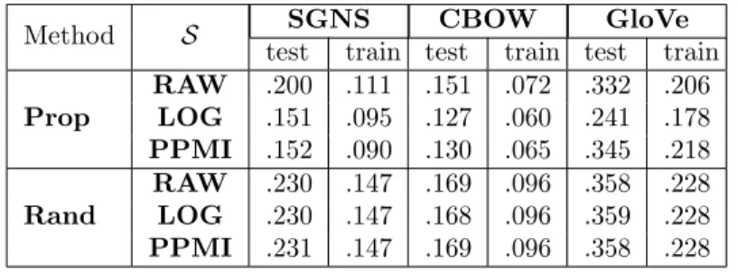
In Table 2, we compare the proposed method (Prop) against a random projection 315
baseline (Rand), where we project thed-dimensional source embeddings onto a 316
p-dimensional space using a random projection matrix,R∈Rd×p, in which each 317
element is randomly sampled from a standard (zero mean and unit variance) Gaussian 318
distribution. From Table 2, we see that both train and test error values for the 319
proposed method is smaller than that of the corresponding random projection. This 320
result shows that the proposed linear transformation learning method outperforms the 321
random projection baseline in both fitting the train word embeddings as well as 322
predicting the test word embeddings. 323
When we use the proposed method to learn linear transformations, among the three 324
counting-based embedding methodsLOGgives the smallest test error for all 325
prediction-based target embedding methods, followed byPPMI, which has a tendency 326
to over-estimate rare co-occurrences. In particular,RAWhas the largest test error 327
when predicting test word embeddings learnt using SGNSandCBOW. This result 328
shows that some form of a co-occurrence weighting method is necessary with 329
counting-based embeddings, if they are to be linearly transformed to prediction-based 330
embeddings. Interestingly,LOGperforms best withGloVe, which can be seen as 331
factorizing a co-occurrence matrix containing the logarithms of the global co-occurrence 332
counts [21]. As forSGNS, which is shown to be factorizing a matrix with shifted PPMI 333
values [20], we do not see any significant differences between test errors reported for 334
LOGandPPMI. 335
LOGas the co-occurrence weighting method for the counting-based word 336
embedding method produces the lowest test prediction error with all of the 337
prediction-based word embeddings. BothSGNSandCBOWare log bi-linear models. 338
The logarithm of the co-occurrence probabilities estimated using those models are 339
proportional to the inner-product between the corresponding word embeddings. By 340
considering the log co-occurrences in the counting-based word embeddings, we can 341
better approximate the linearities present in those prediction-based embedding spaces. 342
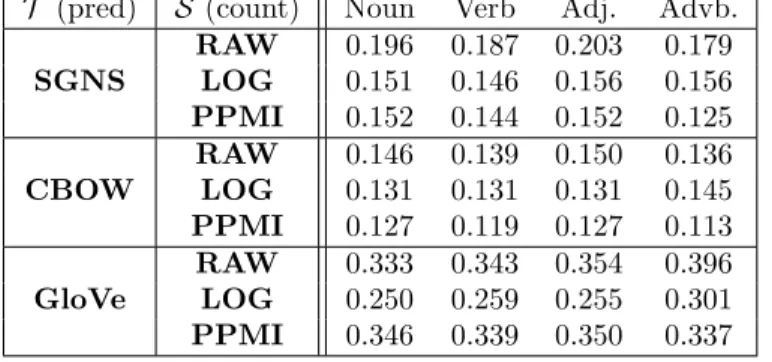
To study the prediction error for different POS categories, we classify each test word 343
Table 1. The hyperparameters used in the prediction tasks. T (pred) S (count) λ π SGNS RAW 10−4 2 LOG 10−4 64 PPMI 10−4 16 CBOW RAW 10−4 16 LOG 10−5 64 PPMI 10−4 16 GloVe RAW 10−5 1 LOG 10−5 32 PPMI 10−2 16
Table 2. Train and test RMSE values when predicting target embeddings (SGNS,
CBOW,GloVe) using different source embeddings (RAW,LOG,PPMI).
Method S SGNS CBOW GloVe
test train test train test train
Prop RAW .200 .111 .151 .072 .332 .206 LOG .151 .095 .127 .060 .241 .178 PPMI .152 .090 .130 .065 .345 .218 Rand RAW .230 .147 .169 .096 .358 .228 LOG .230 .147 .168 .096 .359 .228 PPMI .231 .147 .169 .096 .358 .228
POS category assigned to the first-ranked sense of that word in the WordNet 345
(https://wordnet.princeton.edu/). Next, we compute test error over the words 346
classified to each of the four POS categories as shown in Table 3. Although there are 347
slight variations in the prediction errors across different POS categories, an analysis of 348
variance (ANOVA) test shows that the differences to be statistically insignificant. 349
Therefore, we are unable to find any significant differences between the POS types. 350
Fig 1. Relationship between word frequency, reconstruction error (train RMSE), rank of the target word in list of nearest neighbours (NBRank) computed using the projected embeddings, and the number of senses according to the WordNet for each word. A
linear transformation is learnt betweenLOGsource embedding andGloVetarget
embedding using the proposed method.
Fig 1 shows the distributions of (a) the logarithm of the word frequency, (b) 351
reconstruction error (i.e. training RMSE), (c) rank of the target word in the list of 352
nearest neighbours computed using the projected embeddings, and (d) the number of 353
word senses. 354
For a word w∈ V, we compute the cosine similarity between its projected word 355
embedding, ˆw(T), and the target word embeddings u(T)of each wordu∈ V, and rank
356
uin the descending order of the similarity scores. If the target embedding ofwis 357
ranked higher in this ranked list of nearest neighbours, then we can conclude that the 358
projected embeddings are similar to the actual target embeddings of words. Unlike the 359
RMSE-based evaluation we presented above, the rank of a word in the projected target 360
embedding space considers only the relative position of projected embeddings. Third 361
plot from the top in Fig 1 shows the logarithm of the rank in the nearest neighbour list 362
(log(NBRank)) (vertical axis) against the rank of the word according to its frequency in 363
the corpus (horizontal axis). From Fig 1, we see that for high frequent words (ranks up 364
to 105), the proposed method ranks the target word among the top 100 nearest
Table 3. Testing RMSEs for different counting-based (count.) embeddings as the source, and prediction-based (pred.) as the target for different POS categories.
T (pred) S (count) Noun Verb Adj. Advb.
SGNS RAW 0.196 0.187 0.203 0.179 LOG 0.151 0.146 0.156 0.156 PPMI 0.152 0.144 0.152 0.125 CBOW RAW 0.146 0.139 0.150 0.136 LOG 0.131 0.131 0.131 0.145 PPMI 0.127 0.119 0.127 0.113 GloVe RAW 0.333 0.343 0.354 0.396 LOG 0.250 0.259 0.255 0.301 PPMI 0.346 0.339 0.350 0.337 neighbours. 366
We counted the number of word senses for each word in the WordNet to determine 367
the number of word senses per word. Words that do not appear in the WordNet are 368
ignored in this analysis. In the bottom plot in Fig 1, we show the number of different 369
senses of a word in the vertical axis, whereas the words are ranked by the number of 370
senses they have in the horizontal axis. From Fig 1, we see that except for a small 371
number of common words such as articles and prepositions placed at the first few 372
hundred words in the distribution, our proposed method accurately reconstructs the 373
originalGloVeembeddings with small reconstruction errors, for a range of words. 374
Interestingly, even for polysemous words for which multi-prototype embeddings [29, 30] 375
must be learnt can nevertheless be linearly transformed using the proposed method. 376
Similar distributions were obtained withSGNSandCBOWas the target embeddings. 377
4.2
Predicting Word Similarity and Analogy
378Fig 2. Spearman correlation coefficients (y-axis) between the cosine similarity scores computed using the learnt word embeddings and human ratings in the benchmark
datasets are shown for theCBOWembeddings as functions over the number of SGD
iterations (x-axis).
Fig 3. Spearman correlation coefficients (y-axis) between the cosine similarity scores computed using the learnt word embeddings and human ratings in the benchmark
datasets are shown for theSGembeddings as functions over the number of SGD
iterations (x-axis).
Fig 4. Spearman correlation coefficients (y-axis) between the cosine similarity scores computed using the learnt word embeddings and human ratings in the benchmark
datasets are shown for theGloVeembeddings as functions over the number of SGD
iterations (x-axis).
To evaluate the amount of word semantics preserved during the linear 379
transformation process, we evaluate the predicted target embeddings in two tasks: 380
semantic similarity measurement, and word analogy detection. Both those tasks are 381
frequently used as benchmarks for evaluating word embedding learning methods [31, 32]. 382
For the similarity measurement task we use seven datasets: Rubenstein-Goodenough 383
Fig 5. Accuracies (y-axis) for solving word analogy problems on the Google dataset (semantic analogies, syntactic analogies, and all analogies including semantic and
syntactic), and max-diff scores on the SemEval dataset are shown for theCBOW
embeddings as functions over the number of SGD iterations (x-axis). CosAdd method is used on the Google dataset to predict the correct answer for the word analogy questions.
Fig 6. Accuracies (y-axis) for solving word analogy problems on the Google dataset (semantic analogies, syntactic analogies, and all analogies including semantic and
syntactic), and max-diff scores on the SemEval dataset are shown for theSG
embeddings as functions over the number of SGD iterations (x-axis). CosAdd method is used on the Google dataset to predict the correct answer for the word analogy questions.
Fig 7. Accuracies (y-axis) for solving word analogy problems on the Google dataset (semantic analogies, syntactic analogies, and all analogies including semantic and
syntactic), and max-diff scores on the SemEval dataset are shown for theGloVe
embeddings as functions over the number of SGD iterations (x-axis). CosAdd method is used on the Google dataset to predict the correct answer for the word analogy questions.
(rw, 2034 word-pairs) [35], Stanford’s contextual word similarities (scws, 2023 385
word-pairs) [16], SimLex-999 (simlex, 999 word-pairs) [36], WordSimilarity-353 dataset 386
(ws, 353 word-pairs) [37], and thementest collection (3000 word-pairs) [38]. 387
Each word-pair in those datasets has a manually assigned similarity score. We 388
compute the cosine similarity, cos( ˆu(T),ˆv(T)), between the predicted target embeddings 389
for the two wordsuandv in a word-pair, and use the Spearman correlation coefficient 390
as the evaluation measure to compare predicted similarity scores against the gold 391
standard ratings. Spearman correlation coefficient ranges in [−1,1], and high values 392
indicate a better agreement of the predicted target embeddings with the human notion 393
of semantic similarity. 394
Figs 2, 3, and 4 show the Spearman correlation coefficients for the similarity 395
predictions made using a linear transformation learnt between the counting-based 396
source embeddingLOG, and the three prediction-based target embeddings respectively 397
CBOW,SGNS, andGloVe. The level of correlation obtained by the original target 398
embedding is shown as a dashed horizontal line in each subplot, whereas the 399
performance of the linear transformation afterπnumber of SGD iterations is shown as 400
a solid line. Overall, we see that the correlation coefficients increase withπ, reaching 401
the level of the original prediction-based embeddings after 500 iterations. Therefore, 402
with a sufficiently large number of SGD iterations, the proposed method can learn 403
linear transformations that capture almost all the word semantics encoded in the 404
original prediction-based target embeddings. We use the Google word analogy 405
dataset [19], consisting of semantic(8869 questions) andsyntactic(10675 questions) 406
proportional analogies, and the SemEval 2012 Task 2 dataset (SemEval, 79 407
categories) [39] to evaluate the ability to solve word-analogy problems by the proposed 408
linear transformation learning method. In Figs 5, 6, and 7, we report word analogy 409
solving accuracies for the CosMult method that has shown to produce the best 410
results [40] respectively forCBOW,SG, andGloVe embeddings. 411
Figs 5, 6, and 7 show the scores (percentage of the correctly answered analogy 412
questions on the Google dataset, and the correlation score computed using the official 413
evaluation tool for the SemEval dataset) for the different methods under varying 414
numbers of SGD iterations. Likewise in the semantic similarity experiment, here too we 415
see that with sufficiently large numbers of SGD iterations, the linear transformations 416
target embeddings. Although for many other tasks and projected embeddings the 418
performance is lower compared to the original target embeddings, surprisingly, in a few 419
tasks (semanticandSemEval forCBOW, andSemEval forGloVe), the 420
performance is even better than the original embeddings. This tells us that the original 421
embedding is not necessarily optimal, and our proposed method can learn better 422
embeddings in some cases. One possible reason for this improvement could be because 423
of the`2 regularisation and SGD learning, which prevent overfitting to the original 424
embedding space. 425
4.3
Visualising the Learnt Projections
426Projection matrixCprojects counting-based source embeddings to prediction-based 427
target embeddings. In counting-based embeddings, each dimension is explicitly 428
annotated with a single word representing some semantic concept, whereas in 429
prediction-based embeddings the semantics of each dimension remain implicit. 430
Therefore, the projection matrix Ccan be thought of as a mapping between these two 431
explicit and implicit embedding spaces. To visualise this relationship, we compute the 432
heatmap for some selected rows ofC, corresponding to different context words that 433
appear as dimensions in the counting-based source word embeddings. If the mapping 434
between the two embedding spaces is accurately learnt, we would expect the words that 435
belong to the same class to have the same active dimensions. 436
Following prior work on word representation learning [41, 42], in Figs 8 and 9 show 437
the heatmaps respectively forfruits vs. colours, andanimals vs. countries. From both 438
figures we see that dimensions of the prediction-based embeddings (shown in the 439
horizontal axis) that correspond to the dimensions of the counting-based embeddings 440
(shown in the vertical axis) are different for each context word compared. Note that the 441
ordering of dimensions in each axis is arbitrary and we have used different permutations 442
in each figure to emphasise the association. 443
Fig 8. Heatmap for the projections for fruits vs. colours.
The heatmaps shown in Figs 8 and 9 can be considered as aninterpretation of the 444
dimensions in the counting-based embedding in terms of the dimensions in the 445
prediction-based embedding. We see from the two figures that the same latent 446
dimension in the prediction-based embedding is associated with multiple dimensions in 447
the counting-based embedding. Considering that the dimensionality of the 448
prediction-based embedding (ca. 300) is much smaller than that of the counting-based 449
embedding (ca. 434k), it is natural that a single latent dimension must encode a 450
broader class of semantics represented by multiple dimensions in the counting-based 451
embedding if the two embeddings to capture the same information. Simply ranking 452
dimensions in the counting-based embedding by the values of the elements inC is 453
inadequate to obtain meaningful associations because elements inC can be both 454
positive as well as negative. More advance alignment techniques such as bipartite 455
graph-matching using max-flow methods could be useful here. 456
5
Conclusions
457We proposed a method to learn linear transformations between several counting-based 458
and prediction-based word embeddings. Our proposed method does not depend on the 459
underlining word embedding learning algorithm, hence applicable when finding a linear 460
Fig 9. Heatmap for the projections for animals vs. countries.
particularly attractive because the proposed method can be used as a post-processing 462
analysis tool for aligning the dimensions between different word embeddings. 463
We specifically considered the scenario where we would like to find a linear 464
transformation between prediction-based word embeddings where the dimensions are 465
implicit and randomly initialised, and counting-based word embeddings where the 466
dimensions are explicitly annotated with words. This mapping is useful for providing an 467
interpretation for the implicit dimensions in prediction-based word embeddings using 468
the explicit dimensions in the counting-based word embeddings. It shows that each 469
context word in the counting-based embedding can be associated with a subset of the 470
dimensions in the prediction-based embedding. 471
Our experimental results show that counting-based embeddings of most words can 472
be linearly projected to the vector space spanned by the prediction-based word 473
embeddings. This result is important given that the two types of word embeddings have 474
shown different performances in different tasks, and prior work analysing those 475
differences [1, 10] have hinted at the close relationship between the two types of 476
embeddings. Moreover, experimental results on similarity and analogy benchmarks show 477
that most of the semantic information in the target embeddings can be captured by the 478
proposed method. Visualisations of the projections learnt by the proposed method for 479
different word classes show that indeed the learnt projections demonstrate a high-level 480
of structure organised by the prototypical semantics represented by those word classes. 481
Our work open up several interesting future research directions to the NLP 482
community. 483
• Although linear transformations are simple to interpret and efficient to compute 484
over large vocabularies, it is by no means the only possible transformation 485
between two word embedding spaces. Nonlinear transformations can capture 486
richer relationships between vector spaces as demonstrated repeatedly by the 487
recent successes of deep neural networks. A natural next step would be to explore 488
the possibilities of learning a nonlinear transformation between counting-based 489
and prediction-based word embedding spaces. 490
• The linear transformation we have learnt using our proposed method is a global 491
transformation that applies to all word embeddings equally. However, as evident 492
by the numerous uses of distributional hypothesis that postulates the meaning of 493
a word can be estimated simply by looking at its nearest neighbours, there is a 494
high degree of locality in natural language semantic spaces. Considering this 495
observation, another research direction would be to learn locally-linear 496
transformations [43] between word embedding spaces. 497
• Our analysis shows the existence of a linear transformation at macro-level across 498
different classes of words such as by frequency, level of ambiguity, and 499
part-of-speech. However, it remains an interesting open question as to what 500
specific words can be linearly transformed and to what extent. Such a micro-level 501
analysis would reveal further insights into the relationships between 502
counting-based and prediction-based embeddings. 503
• Equation (1) can be extended to incorporate multiple target embeddings by 504
adding loss terms corresponding to the projection between each target embedding 505
and the single source embedding. The transformation matrixCcan then be 506
shared across the different loss terms such that we learn a single consistent linear 507
• Our proposed method can be used to find a liner transformation betweenany two 509
embeddings, not limited to a counting-based source embedding and a 510
prediction-based target embedding. This is useful to quantitatively understand 511
how one set of embeddings is related to another set of embeddings created using 512
different embedding learning methods, different resources, or different random 513
initialisations of the same algorithm. Two embedding learning algorithms might 514
appear to be different in the objectives that they optimise for and/or the 515
optimisation techniques that they use. However, when trained on the same 516
resources, they might produce similar embeddings, different only by a linear 517
transformation. Our proposed method can be used as a tool to further investigate 518
the embeddings learnt by different embedding learning algorithms. As a special 519
case of such an analysis, the coefficients of the projection matrix provides an 520
interpretation for the alignment between dimensions in the source and target 521
embeddings. The visualisations shown in the paper are a first attempt at such an 522
analysis. We plan to peruse those research directions in our future work. 523
References
1. Baroni M, Dinu G, Kruszewski G. Don’t count, predict! A systematic comparison of context-counting vs. context-predicting semantic vectors. In: Proc. of ACL; 2014. p. 238–247. Available from:
http://www.aclweb.org/anthology/P/P14/P14-1023.
2. Turney PD, Pantel P. From Frequency to Meaning: Vector Space Models of Semantics. Journal of Aritificial Intelligence Research. 2010;37:141 – 188. 3. Pennington J, Socher R, Manning CD. GloVe: global vectors for word
representation. In: Proc. of EMNLP; 2014. p. 1532–1543.
4. Mikolov T, Chen K, Dean J. Efficient estimation of word representation in vector space. In: Proc. of International Conference on Learning Representations; 2013. 5. Ling W, Dyer C, Black AW, Trancoso I. Two/Too Simple Adaptations of
Word2Vec for Syntax Problems. In: Proceedings of the 2015 Conference of the North American Chapter of the Association for Computational Linguistics: Human Language Technologies. Denver, Colorado: Association for Computational Linguistics; 2015. p. 1299–1304. Available from:
http://www.aclweb.org/anthology/N15-1142.
6. Socher R, Perelygin A, Wu J, Chuang J, Manning CD, Ng A, et al. Recursive Deep Models for Semantic Compositionality Over a Sentiment Treebank. In: Proc. of EMNLP; 2013. p. 1631–1642. Available from:
http://www.aclweb.org/anthology/D13-1170.
7. Passos A, Kumar V, McCallum A. Lexicon Infused Phrase Embeddings for Named Entity Resolution. In: Proc. of CoNLL; 2014. p. 78–86.
8. Woodsend K, Lapata M. Distributed Representations for Unsupervised Semantic Role Labeling. In: Proc. of EMNLP; 2015. p. 2482–2491. Available from:
http://aclweb.org/anthology/D15-1295.
9. Zou WY, Socher R, Cer D, Manning CD. Bilingual Word Embeddings for Phrase-Based Machine Translation. In: Proc. of EMNLP; 2013. p. 1393–1398.
10. Levy O, Goldberg Y, Dagan I. Improving Distributional Similarity with Lessons Learned from Word Embeddings. Transactions of Association for Computational Linguistics. 2015;3:211–225.
11. Maas AL, Daly RE, Pham PT, Huang D, Ng AY, Potts C. Learning Word Vectors for Sentiment Analysis. In: ACL; 2011. p. 142 – 150.
12. Bollegala D, Maehara T, ichi Kawarabayashi K. Unsupervised Cross-Domain Word Representation Learning. In: Proc. of ACL; 2015. p. 730 – 740. 13. Turian J, Ratinov L, Bengio Y, Roth D. A preliminary evaluation of word
representations for named-entity recognition. In: Proc. of NIPS GRLL Workshop; 2009.
14. Al-Rfou R, Kulkarni V, Perozzi B, Skiena S. Polyglot-NER: Massive Multilingual Named Entity Recognition. In: Proceedings of 2015 SIAM International
Conference on Data Mining; 2015.
15. Iacobacci I, Pilehvar MT, Navigli R. SensEmbed: Learning Sense Embeddings for Word and Relational Similarity. In: Proceedings of the 53rd Annual Meeting of the Association for Computational Linguistics and the 7th International Joint Conference on Natural Language Processing (Volume 1: Long Papers). Beijing, China: Association for Computational Linguistics; 2015. p. 95–105. Available
from: http://www.aclweb.org/anthology/P15-1010.
16. Huang EH, Socher R, Manning CD, Ng AY. Improving Word Representations via Global Context and Multiple Word Prototypes. In: Proc. of ACL; 2012. p. 873–882.
17. Bollegala D, Maehara T, ichi Kawarabayashi K. Embedding Semantic Relationas into Word Representations. In: Proc. of IJCAI; 2015. p. 1222 – 1228.
18. Labutov I, Lipson H. Re-embedding Words. In: Proc. of ACL (short papers); 2013. p. 489 – 493.
19. Mikolov T, Sutskever I, Chen K, Corrado GS, Dean J. Distributed
representations of words and phrases and their compositionality. In: Proc. of NIPS; 2013. p. 3111–3119.
20. Levy O, Goldberg Y. Neural Word Embedding as Implicit Matrix Factorization. In: Proc. of NIPS; 2014.
21. Keerthi SS, Schanbel T, Khanna R. Towards Better Understanding of Predict and Count Models. arXiv. 2015;0.
22. Arora S, Li Y, Liang Y, Ma T, Risteski A. RAND-WALK: A latent variable model approach to word embeddings. Transactions of Association for Computational Linguistics. 2016; p. to appear.
23. Faruqui M, Dyer C. Non-distributional Word Vector Representations. In: Proc. of ACL; 2015. p. 464–469.
24. Mitchell J, Steedman M. Orthogonality of Syntax and Semantics within Distributional Spaces. In: Proc. of ACL; 2015. p. 1301–1310.
25. Kedem D, Tyree S, Weinberger K, Sha F, Lanckriet G. Non-linear Metric Learning. In: Proc. of NIPS; 2012. p. 2582–2590. Available from:
26. Tikhonov A. Solution of incorrectly formulated problems and the regularization method. In: Soviet Math. Dokl.. vol. 5; 1963. p. 1035–1038.
27. Duchi J, Hazan E, Singer Y. Adaptive Subgradient Methods for Online Learning and Stochastic Optimization. Journal of Machine Learning Research.
2011;12:2121–2159.
28. Gutmann MU, Hyv¨arinen A. Noise-Contrastive Estimation of Unnormalized
Statistical Models, with Applications to Natural Image Statistics. Journal of Machine Learning Research. 2012;13:307–361.
29. Neelakantan A, Shankar J, Passos A, McCallum A. Efficient Non-parametric Estimation of Multiple Embeddings per Word in Vector Space. In: Proc. of EMNLP; 2014. p. 1059–1069. Available from:
https://www.youtube.com/watch?v=EeBj4TyW8B8&feature=youtu.be.
30. Reisinger J, Mooney RJ. Multi-Prototype Vector-Space Models of Word Meaning. In: Proc. of HLT-NAACL; 2010. p. 109–117.
31. Schnabel T, Labutov I, Mimno D, Joachims T. Evaluation methods for unsupervised word embeddings. In: Proc. of EMNLP; 2015. p. 298–307.
Available from: http://aclweb.org/anthology/D15-1036.
32. Tsvetkov Y, Faruqui M, Ling W, Lample G, Dyer C. Evaluation of Word Vector Representations by Subspace Alignment. In: Proc. of EMNLP; 2015. p.
2049–2054. Available from: http://aclweb.org/anthology/D15-1243.
33. Rubenstein H, Goodenough JB. Contextual Correlates of Synonymy. Communications of the ACM. 1965;8:627–633.
34. Miller G, Charles W. Contextual correlates of semantic similarity. Language and Cognitive Processes. 1998;6(1):1–28.
35. Luong MT, Socher R, Manning CD. Better Word Representations with Recursive Neural Networks for Morphology. In: CoNLL; 2013.
36. Hill F, Reichart R, Korhonen A. SimLex-999: Evaluating Semantic Models With (Genuine) Similarity Estimation. Computational Linguistics. 2015;41(4):665–695. 37. Finkelstein L, Gabrilovich E, Matias Y, Rivlin E, z Solan, Wolfman G, et al.
Placing Search in Context: The Concept Revisited. ACM Transactions on Information Systems. 2002;20:116–131.
38. Bruni E, Boleda G, Baroni M, Tran NK. Distributional Semantics in Technicolor. In: Proc. of ACL; 2012. p. 136–145. Available from:
http://www.aclweb.org/anthology/P12-1015.
39. Jurgens DA, Mohammad S, Turney PD, Holyoak KJ. Measuring Degrees of Relational Similarity. In: Proc. of SemEval; 2012.
40. Levy O, Goldberg Y. Linguistic regularities in sparse and explicit word representations. In: CoNLL; 2014.
41. Yogatama D, Faruqui M, Dyer C, Smith NA. Learning Word Representations with Hierarchical Sparse Coding. In: arxiv; 2014.
42. Faruqui M, Tsvetkov Y, Yogatama D, Dyer C, Smith NA. Sparse Overcomplete Word Vector Representations. In: Proceedings of the 53rd Annual Meeting of the Association for Computational Linguistics and the 7th International Joint Conference on Natural Language Processing (Volume 1: Long Papers). Beijing, China: Association for Computational Linguistics; 2015. p. 1491–1500. Available
from: http://www.aclweb.org/anthology/P15-1144.
43. Saul LK, Roweis ST. Think Globally, Fit Locally: Unsupervised Learning of Low Dimensional Manifolds. Journal of Machine Learning Research. 2003;4:119–115.