A Testing Based Extraction Algorithm for Identifying Significant Communities in Networks

USF Scholarship: a digital repository @ Gleeson Library |

Geschke Center

Mathematics

College of Arts and Sciences

2014

A Testing Based Extraction Algorithm for

Identifying Significant Communities in Networks

James D. Wilson

University of San Francisco, [email protected]

Simi Wang

Peter J. Mucha

Shankar Bhamidi

Andrew B. Nobel

Follow this and additional works at:

http://repository.usfca.edu/math

Part of the

Mathematics Commons

This Article is brought to you for free and open access by the College of Arts and Sciences at USF Scholarship: a digital repository @ Gleeson Library | Geschke Center. It has been accepted for inclusion in Mathematics by an authorized administrator of USF Scholarship: a digital repository @ Gleeson Library | Geschke Center. For more information, please [email protected].

Recommended Citation

Wilson, J. D., Wang, S., Mucha, P.J., Bhamidi, S., & Nobel, A.B. (2014). A testing based extraction algorithm for identifying significant communities in networks. Annals of Applied Statistics, Vol. 8, No. 3, 1853-1891. http://dx.doi.org/10.1214/14-AOAS760

arXiv:1308.0777v4 [cs.SI] 3 Dec 2014

c

Institute of Mathematical Statistics, 2014

A TESTING BASED EXTRACTION ALGORITHM FOR

IDENTIFYING SIGNIFICANT COMMUNITIES IN NETWORKS1

By James D. Wilson, Simi Wang, Peter J. Mucha2, Shankar Bhamidi and Andrew B. Nobel

University of North Carolina at Chapel Hill

A common and important problem arising in the study of net-works is how to divide the vertices of a given network into one or more groups, called communities, in such a way that vertices of the same community are more interconnected than vertices belonging to different ones. We propose and investigate a testing based commu-nity detection procedure called Extraction of Statistically Significant Communities (ESSC). The ESSC procedure is based on p-values for the strength of connection between a single vertex and a set of ver-tices under a reference distribution derived from a conditional con-figuration network model. The procedure automatically selects both the number of communities in the network and their size. Moreover, ESSC can handle overlapping communities and, unlike the major-ity of existing methods, identifies “background” vertices that do not belong to a well-defined community. The method has only one pa-rameter, which controls the stringency of the hypothesis tests. We in-vestigate the performance and potential use of ESSC and compare it with a number of existing methods, through a validation study using four real network data sets. In addition, we carry out a simulation study to assess the effectiveness of ESSC in networks with various types of community structure, including networks with overlapping communities and those with background vertices. These results sug-gest that ESSC is an effective exploratory tool for the discovery of relevant community structure in complex network systems. Data and software are available at _{http://www.unc.edu/~jameswd/research.}

html.

Received September 2013; revised May 2014.

1_{Supported in part by NSF Grants DMS-09-07177, DMS-13-10002, DMS-06-45369,}

DMS-11-05581 and SES-1357622.

2_{Supported in part by the James S. McDonnell Foundation 21st Century Science}

Initiative—Complex Systems Scholar Award Grant 220020315.

Key words and phrases. Community detection, networks, extraction, background, mul-tiple testing.

This is an electronic reprint of the original article published by the Institute of Mathematical StatisticsinThe Annals of Applied Statistics,

2014, Vol. 8, No. 3, 1853–1891. This reprint differs from the original in pagination and typographic detail.

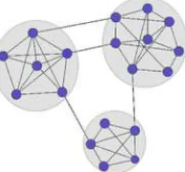
1. Introduction. The study of networks has been motivated by, and made significant contributions to, the modeling and understanding of com-plex systems. Networks are used to model the relational structure between individual units of an observed system. In the network setting, vertices rep-resent the units of the system and edges are placed between vertices that are related in some way. Network-based models have been used in a variety of disciplines: in biology to model protein-protein and gene–gene interactions; in sociology to model friendship and information flow among a group of in-dividuals; and in neuroscience to model the relationship between the organi-zation and function of the brain. In many of these applications, the vertices of the network under study can naturally be subdivided into communities. Informally, a community is a group of vertices that are more connected to each other than they are to the remainder of the network. More rigorous definitions quantify this notion of differential connection in different ways. Figure1 illustrates a network with three disjoint communities.

The problem of dividing the vertices of a given network into well-defined communities is known as community detection. Community detection has become increasingly popular, as communities have been found to identify important and useful features of many complex systems. Community detec-tion has been studied by researchers in a variety of fields, including statistics, the social sciences, computer science, physics and applied mathematics, and a diverse set of community detection algorithms have been developed [see Fortunato (2010), Porter, Onnela and Mucha (2009) for reviews].

Existing community detection methods capture different types of commu-nity structure. The simplest commucommu-nity structure, and the one most com-monly studied, is a hard partitioning, in which each vertex of the network is assigned to one and only one community, and the collection of communities together form a partition of the network [e.g., Newman and Girvan (2004), Ng, Jordan and Weiss (2002), Snijders and Nowicki (1997)]. Another class of community structure allows overlapping communities [see Xie, Kelley and Szymanski (2011) for a recent review], in which the collection of communities together form a cover of the network. Broadly speaking, most community detection methods produce one of these types of structures.

Community detection has been successful in understanding a wide va-riety of complex systems. In addition to the numerous examples cited in the aforementioned reviews, community detection methods have recently been profitably applied to protein interaction networks [Lewis et al. (2010)], functional brain activity [Bassett et al. (2011)], social media [Papadopou-los et al. (2012)] and mobile phone data [Muhammad and Van Laerhoven (2013)], as well as social groups [Greene, Doyle and Cunningham (2010), Miritello, Moro and Lara (2011), Onnela et al. (2011)].

The majority of existing community detection methods make the assump-tion that every vertex within an observed network belongs to at least one community. Though many networks can be appropriately divided into a par-tition (or cover) of communities, some large and heterogeneous networks do not fit into this framework. For example, consider the Enron email network from Leskovec et al. (2009) where edges represent the email correspondence (sent or received) between email accounts in 2001. The network contains many (on the order of 10K) email accounts outside of Enron and relatively few (on the order of 1K) email accounts from employees at Enron. The outside email accounts, many of which are spam email accounts, are not preferentially attached to any group of employees and thereby do not be-long to a well-defined community. From this example and several others that we investigate in Section4, we will see that many real networks contain ver-tices that do not have strong connections toany community. Informally, we call vertices that are not preferentially connected to any community back-ground vertices, as they act as a background against which more standard community structures may be detected.

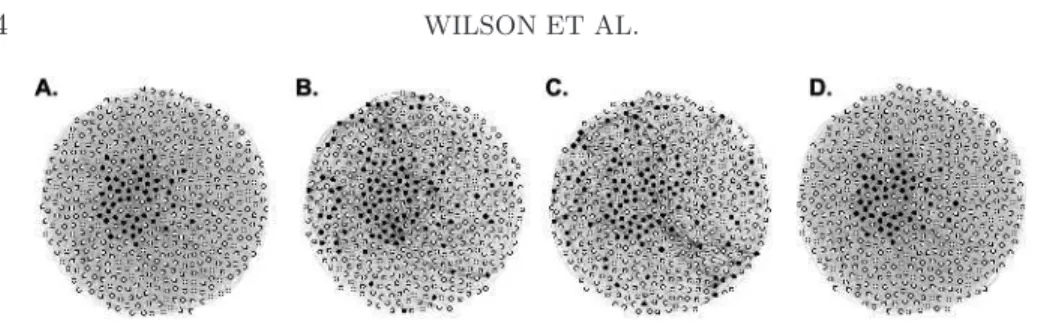
In networks where background vertices are present, partitioning and cov-ering methods typically assign them to more tightly connected communities. To illustrate this, we generated a 500 node toy network with a single commu-nity of size 50, whose vertices are linked independently with probability 0.5; the remaining vertices are background and are linked to all vertices in the network independently with probability 0.05. We ran two popular detection methods—the modularity based algorithm of Newman and Girvan (2004) and the normalized Spectral algorithm of Ng, Jordan and Weiss (2002)— and found two disjoint communities. We considered the community that most closely matched the true embedded community and found, as shown in Figure2, that both methods included many background vertices.

Also shown in Figure 2 is the result of applying the ESSC method in-troduced in this paper. ESSC accurately identifies the embedded commu-nity and the background, and separates one from the other. Although there are methods in multivariate clustering to capture background [Ester et al. (1996), Hinneburg and Keim (1998)], only a few recent papers, for example, Zhao, Levina and Zhu (2011), Lancichinetti et al. (2011), consider back-ground in the context of community detection.

Fig. 2. (A)A toy network that contains one significantly connected community—colored in black—and many sparsely connected background vertices. (B) The partition given by the GenLouvain modularity optimization method.(C) The partition given by normalized Spectral clustering. (D) The extracted community found by the proposed method ESSC, which separates and distinguishes the embedded community from the background.

In this paper we propose and study a testing based community detec-tion algorithm, called Extracdetec-tion of Statistically Significant Communities (ESSC), that is capable of identifying both background vertices and overlap-ping communities. The core of the algorithm is an iterative search procedure that identifies statistically stable communities. In particular, the search pro-cedure uses tail probabilities derived from a stochastic configuration model based on the observed network in order to assess the strength of the connec-tion between a single vertex and a candidate community. Updating of the candidate community is carried out using ideas from multiple testing and false discovery rate control.

The only free parameter in the ESSC algorithm is a false discovery rate threshold that is used in the update step of the iterative search procedure. The number of detected communities, their overlap (if any) and the size of the background are handled automatically, without user input. In practice, the output of ESSC is not overly sensitive to the threshold parameter; see the AppendixD for more details.

1.1. Notation. For ease of discussion throughout the remainder of this paper, we first introduce some notation. Let G= (V, E) be an undirected multigraph with vertex setV = [n] ={1, . . . , n}and edge multisetE contain-ing all (unordered) pairs {i, j} such that there is an edge between vertices

i and j in G, allowing repetitions for multiple edges. Let d(u) denote the degree of a vertexu, and letd={d(1), . . . , d(n)}denote the degree sequence of G. Let B⊂[n] denote a subset of vertices inG. Indices onB are simply used for specification throughout. Write Π for a partition of the vertex set [n] (Π =B1∪B2∪ · · · ∪Bk,k≥1). In many cases, detection methods seek a

partition (or cover) through optimizing a specified quality or score function, which we will denote as S(·). It is important to note that the score may be global, in which caseS(·) measures the quality of an entire partition, or local, in which caseS(·) measures the quality of a potential community. We

will use Go to denote an observed graph and Gb for a stochastic model on the vertex set [n].

1.2. Related work. There is an extensive literature on the development and analysis of community detection methods. In this section we give an overview of this literature. For recent surveys describing community detec-tion methods, see Fortunato (2010), Porter, Onnela and Mucha (2009) or Goldenberg et al. (2010). In Section3we describe in more detail the methods to which we compare ESSC.

Many of the earliest community detection methods approach network clustering from a graph-theoretic standpoint. Relying on a prespecified inte-gerk, these methods seek the partition ofk communities that minimize the number of edges between communities. The optimal partition of this crite-rion is known as the partition of min-cut and max-flow [Goldberg and Tarjan (1988)], where the cut of a community specifies the number of edges from the community to the rest of the network. Unfortunately, min-cut methods often result in many singleton communities. To address this issue, the cut of a community can be normalized by either the community size, resulting in the ratio-cut criterion [Wei and Cheng (1989)], or by the total degree of the community, giving the normalized-cut criterion [Shi and Malik (2000)].

When k >2, the task of finding the partition that satisfies any of these cut

criterions is NP-hard. Spectral clustering methods [Krzakala et al. (2013), Ng, Jordan and Weiss (2002)] find an approximate solution to the norm-cut criterion by appealing to spectral properties of the graph Laplacian. Spectral clustering methods can be applied to either nonnetwork multivariate data or directly to relational network data.

Another class of community detection methods seek community structure by comparing the observed network Go = ([n], Eo) with an unstructured stochastic network on the same vertex set Gbnull= ([n],Eˆnull). A stochastic

networkGbnulldescribes the probabilities of edge connection between all pairs

of vertices in [n] given that each pair was connected at random. Detection methods of this class seek the partition ofGowhose clustering most deviates from what is expected under Gbnull. Modularity methods [see, e.g., Blondel

et al. (2008), Clauset, Newman and Moore (2004), Newman (2006), Mucha et al. (2010)] are a popular subset of this class. Modularity methods seek the partition whose communities’ fraction of observed edges are furthest from the fraction of edges expected under Gbnull, that is, the partition Π that

maximizes Smod(Π) = 1 2|Eo| k X ℓ=1 X i,j∈Bℓ I_{({i, j} ∈Eo)−γ}E X i,j∈Bℓ I_{({i, j} ∈E}ˆ_null) ,

where γ >0 is a resolution parameter that controls the size of discovered communities. In many cases, γ is treated as one, however, this parameter

can be tuned in a data-driven fashion. There are many choices for a refer-ence stochastic network. For instance, in the case of the Newman–Girvan modularity [Newman and Girvan (2004)], Gbnull is specified as the

configu-ration model [Molloy and Reed (1995)] under which the degree sequence of

Go is maintained. In this caseE(Pi,j∈BℓI({i, j} ∈

ˆ

Enull)) isdo(i)do(j)/2|Eo|. Our proposed method ESSC also relies upon the configuration model as a reference stochastic network.

An alternative class of community detection methods estimate the com-munity structure of a network by fitting a structured stochastic network

b

Gstruct= ([n],Eˆstruct) to the observed data Go. Here, Gbstruct describes

ran-dom assignments of edges conditional on stochastic community (or block) structure on the vertex set [n]. Formally,Gbstruct is a parametric model whose

parameters describe the community labels of each vertex and potentially the topological properties of the network (e.g., the degree distribution of the network). Given an observed network Go and a prespecified integer k, a structured network (with parameters Θ) is fit to Go by maximizing the likelihood function describing Θ: L(Θ|Go, k). A recent review of structured network models is provided by Goldenberg et al. (2010). One of the most popular network models of this type is the stochastic block model [Holland, Laskey and Leinhardt (1983), Snijders and Nowicki (1997), Nowicki and Sni-jders (2001)]. Under this model, vertices are assigned labels taking values in

{1, . . . , k}according to probabilitiesπ= (π1, . . . , πk). Conditional on the

ver-tex labels, edge probabilities are given by ak×ksymmetric matrixPwhere thei,jth entry ofP gives the probability of an edge between community i

and j. Block models are fit to Go by maximizing the corresponding likeli-hoodL(Θ = (P, π)|Go, k). Other examples of structured stochastic networks include latent variable models [Hoff, Raftery and Handcock (2002), Hand-cock, Raftery and Tantrum (2007)] and mixed membership models which are flexible to overlapping communities [Airoldi et al. (2008), Ball, Karrer and Newman (2011)].

Recently, there has been significant progress in the development of fast and efficient algorithms for fitting stochastic block models. The authors of Decelle et al. (2011) describe an algorithm that estimates block structure of a degree-corrected block model in time linear in the number of vertices. Their algorithm is based on a powerful heuristic of belief propagation from statistical physics. See, for example, M´ezard and Montanari (2009) for a survey level treatment of belief propagation and a variety of applications. In the context of sparse stochastic block models, these techniques have been shown to be near optimal in estimating the underlying communities [Krza-kala et al. (2013)], at least in the balanced regime where both communities are of equal size. A sublinear algorithm based on the pseudo-likelihood of the sparse block model is described in Amini et al. (2013) wherein block labels

are shown to be consistent in the size of network. Finally, recent nonpara-metric representations of the block model through dense graph limits, or graphons [Airoldi, Costa and Chan (2013)] and network histograms [Olhede and Wolfe (2013)] provide promising new directions for the understanding and estimation of block models.

Another subclass of community detection methods are the so-called ex-traction techniques where communities are extracted one at a time [Zhao, Levina and Zhu (2011), Lancichinetti et al. (2011)]. Rather than search for an optimal partition or cover, these extraction methods seek the strongest connected community sequentially. Extraction methods do not force all ver-tices to be placed in a community and thereby are flexible to loosely con-nected background vertices. ESSC is an extraction method that utilizes the reference distribution of the connectivity of a community based on the con-ditional configuration model.

There are two main approaches currently used to assess the statistical sig-nificance of communities in networks. The first approach, like ESSC, builds upon statistical principles based on features of the observed network itself. The second approach is permutation based in that the significance of com-munity structure is determined based on the results of a prescribed method on many bootstrapped samples of the observed network [see, e.g., Clauset, Moore and Newman (2008), Rosvall and Bergstrom (2010)]. Many theoreti-cal questions remain open for these types of methods, including convergence of bootstrapped samples of networks.

1.3. Organization of the paper. The remainder of this paper is organized as follows. Section 2 is devoted to a detailed description of our proposed algorithm for extraction of statistically significant communities (ESSC), in-cluding motivation and a description of the reference distribution gener-ated from the configuration model. In Section1.2we discuss the competing methods that we use to validate our algorithm in both numerical and real network studies. In Section 4 we apply the ESSC algorithm to four real-world networks. These results provide solid evidence that ESSC performs well in practice, is competitive with (and in some cases arguably superior to) several leading community detection methods, and is effective in captur-ing background vertices. In Section 5 we propose a test bed of benchmark networks for assessing the performance of detection methods specifically on networks with background vertices. To the best of our knowledge, this is the first set of benchmarks proposed for networks of this type. We show that ESSC outperforms existing methods on these background benchmarks. We also show that ESSC performs competitively on standard (nonbackground) benchmark networks with both nonoverlapping and overlapping community structures. We end with a discussion of our work and avenues for future research.

2. The ESSC algorithm.

2.1. Conditional configuration model. LetGobe an observed, undirected network havingnvertices. Though many networks of interest will be simple,

Go may contain self-loops or multiple edges. Assume without loss of gen-erality that Go has vertex set V = [n] ={1,2, . . . , n}. The edge multiset Eo of Go contains all (unordered) pairs {i, j} such that i, j∈[n] and there is a link between vertices iand j inGo, with repetitions for multiple edges. Let

do(u) denote the degree of a vertex u, that is, the number of edges incident onu, and let do={do(1), . . . , do(n)} denote the degree sequence ofGo.

The starting point for our analysis is a stochastic network model that is derived from the degree sequencedo ofGo, specifically, the configuration model associated withdo, which we denote by CM(do) [Bender and Canfield (1978), Bollob´as (1979), Molloy and Reed (1995)]. The configuration model CM(do) is a probability measure on the family of multigraphs with vertex set [n] and degree sequence do that reflects, within the constraints of the degree sequence, a random assignment of edges between vertices.

The configuration model CM(do) has a simple generative form. Initially, each vertexu∈[n] is assigneddo(u) “stubs,” which act as half-edges. At the next stage, two stubs are chosen uniformly at random and connected to form an edge; this procedure is repeated independently until all stubs have been connected. Let Gb= ([n],Eˆ) denote the random network generated by this procedure. Note thatGb may contain self loops and multiple edges between vertices, even if the given networkG is simple.

The configuration model CM(do) is capable of capturing and preserving strongly heterogeneous degree distributions often encountered in real net-work data sets. Importantly, all edge probabilities in the configuration null model are determined solely by the degree sequencedoof an observed graph. As a result, fitting a configuration model does not rely on simulation, rather, estimation only requires the degree sequence of a single observed graph.

Under the configuration model CM(do) there are no preferential connec-tions between vertices, beyond what is dictated by their degrees. As such,

CM(do) provides a reference measure against which we may assess the

sta-tistical significance of the connections between two sets of vertices in the observed networkGo: the more the observed number of cross-edges deviates from the expected number under the model, the greater the significance of the connection between the vertex sets. Let the observed network Go and the random network Gb be as above. Given a vertex u∈[n] and vertex set

B⊆[n], let do(u:B) =X v∈B X e∈Eo I_{(e={u, v})}

denote the number of edges between u and some vertex in B inGo. Define ˆ

d(u:B) as the corresponding number of edges in Gb. Note that ˆd(u:B) is a random variable taking values in the set {0,1, . . . , do(u)}, and that do(u:

B) = ˆd(u:B) =do(u) when B= [n] is the full vertex set. We now state a theorem describing asymptotics for the random variable ˆd(u:B) in the configuration model which will form the basis of the algorithm. Recall that the total variation distance between two probability mass functions p:=

{p(i)}i≥0 andq:={q(i)}i≥0 on the space of natural numbersNis defined by

dTV(p,q) := 1 2 ∞ X i=0 |p(i)−q(i)|.

Theorem 1. Let {do,n}n≥1 be the degree sequences of an observed

se-quence of graphs{Gn

o}n≥1, whereGno is a graph with vertex set [n]and edge

setEo,n. Let{Gbn}n≥1 be the corresponding random graphs on[n]constructed

via the configuration model. LetFnbe the empirical distribution ofdo,n.

As-sume that there exists a cumulative distribution function F on [0,∞) with

0< µ:=RR+x dF(x)<∞ such that Fn w −→F (2.1) and Z R+ x dFn(x)→µ. (2.2)

Fixk≥1. For eachn≥1, letu=un∈[n]be a vertex with degreedo,n(u) =k

and letB=B(n)⊆[n] be a set of vertices. Then the random variabledˆn(u:

B) is approximately Binomial(k, pn(B))in the sense that

dTV( ˆdn(u:B),Bin(k, pn(B)))→0, as n→ ∞. Here pn(B) = P v∈Bdo,n(v) P w∈[n]do,n(w) = 1 2|Eo,n| X v∈B do,n(v), (2.3)

where |Eo,n|is the total number of edges in the graph.

A precise proof of this fact is given in the AppendixA. In light of the fact that the configuration model CM(do) does not contain preferential connec-tions between vertices, the probabilities

p(u:B) =P( ˆd(u:B)≥do(u:B))

(2.4)

can be used to assess the strength of connection between a vertexuand a set of verticesB⊆[n]. In particular, small values ofp(u:B) indicate that there

are more edges between u and B than expected under the configuration model.

If we regard do(u:B) as the observed value of a test statistic that is distributed as ˆd(u:B) under the null model CM(do), then p(u:B) has the form of ap-value for testing the hypothesis thatuis not strongly associated withB.

This testing interpretation ofp(u:B) plays a role in the iterative search procedure that underlies the ESSC method (see below). However, we note that the testing point of view is informal, as the null model CM(do) itself depends on the observed network Go through its degree distribution.

In general, the exact value of the probability p(u:B) in (2.4) may be difficult to obtain. In practice, the ESSC procedure approximates p(u:B) by P(XB≥do(u:B)), where XB has a Binomial(d(u), p(B)) distribution appealing to the result of Theorem1.

2.2. Description of the ESSC algorithm. The core of the ESSC algorithm is an iterative deterministic procedure (Community-Search) that searches for robust, statistically significant communities. Beginning with an initial setB0 of vertices that acts as a seed, the procedure successively refines and

updates B0 using (the binomial approximation of) the probabilities (2.4)

until it reaches a fixed point, that is, a vertex set that is unchanged under updating. The final vertex set identified by the search procedure is a detected community.

The Community-Search procedure is applied repeatedly, using an adap-tively chosen sequence of seed vertices, until it returns an empty community with no nodes. The resulting collectionC of detected communities (omitting repetitions) constitutes the output of the algorithm. The seed setB0 for the

initial run of the search procedure is the vertex of highest degree and all of the vertices adjacent to it. In subsequent runs of the search procedure the seed set B0 is the vertex of highest degree not contained in any previously

detected community and all the vertices adjacent to it, regardless of whether the latter lie in a previously detected community or not.

To simplify what follows, letC1, . . . , CK be the distinct detected commu-nities of Go in C. The background ofGo is defined to be the set of vertices that do not belong to any detected communities:

C∗= Background(Go:C) = [n]

/_[K k=1

Ck.

(2.5)

In principle, the number K of detected communities can range from zero to n. Importantly, K is not fixed in advance, but is adaptively determined by the ESSC algorithm. The identification of detected communities by the

number of discovered communities,K, the presence and extent of overlap is automatic; no prior specification of overlap specific parameters are required. The updates of theCommunity-Search procedure bear further discussion. Consider an ideal setting in which, for each vertexuand vertex setB we can determine, in an unambiguous way, whether or not u is strongly connected to B in Go. Informally, a set of vertices B is a community if the vertices

u∈B have a strong connection with vertices inB, while the verticesu∈Bc do not. Equivalently, B is a community if and only if it is a fixed point of the update rule

S(A) ={u∈[n] such that u is strongly connected with A}

that identifies the vertices having a strong connection with a set of vertices

A⊆[n]. Formally, we may regardS(·) as a map from the power set of [n] to itself. A vertex set B is a fixed point of S(·) if S(B) =B. In order to find a fixed point of the update ruleS(·), we apply the rule repeatedly, starting from a seed set of vertices B0, until a fixed point is obtained. The eventual

termination (and success) of this simple procedure is assured, as the power set of [n] is finite. By the exhaustive or selective considering of appropriate seed sets we can effectively explore the space of fixed points of S(·), and thereby identify communities in Go.

The choice of a seed setBo for theCommunity-Search procedure requires further discussion. As currently implemented, we choose Bo as the neigh-borhood of the highest degree vertex among the vertices lying outside cur-rently extracted communities. Consider the following situation, as pointed out by a referee, where one has two disconnected clusters C, C′ _{such that}

C contains no inherent community structure, for example, an Erd˝os–R´enyi random graph, and C′ _{contains strong community structure, for example,}

a well-differentiated stochastic block model. If the maximal degree of C is larger than C′_{, then ESSC could fail to find the community structure in}

C′_{. To address the above situation, one can run theCommunity-Search}

pro-cedure in parallel across all vertex neighborhoods. In this case, the final communities are the collection of uniquely extracted vertex sets. We found that the situation above did not arise in any of the applications or simula-tions that we investigate in this paper.

In practice, we make use of the probabilities{p(u:B) :u∈[n]}to measure the strength of the connection betweenu∈[n] andB relative to the reference distribution CM(d). In particular, we regardp(u:B) informally as ap-value for testing the null hypothesis HB

u that u is not preferentially connected to

B. Then the task of identifying the vertices u preferentially connected to

B amounts to rejecting a subset of the hypotheses {HB

u :u∈[n]}. This is accomplished in steps 4 and 5 of theCommunity-Searchprocedure, where we make use of an adaptive method of Benjamini and Hochberg [Benjamini and

Hochberg (1995)] to reject a subset of the hypotheses. The rejection method ensures that the expected number of falsely rejected hypotheses divided by the total number of rejected hypotheses (the so-called false discovery rate) is at mostα[see Benjamini and Hochberg (1995) for more details]. A default false discovery rate thresholdαof 5% is common in many applications, and we adopt this value here. Pseudo-code for theCommunity-Search procedure and ESSC algorithm is shown below.

Community-Search Procedure

Given: GraphGo= ([n], Eo); significance level α∈(0,1).

Input: Seed set B0⊆[n].

Initialize:t:=−1,B−1=∅.

Loop (Update): UntilBt+1=Bt 1. t:=t+ 1.

2. Computep(u:Bt) for each u∈[n].

3. Order the nvertices of Go so that p(u1:Bt)≤ · · · ≤p(un:Bt). 4. Letk≥0 be the largest integer such that p(uk:B)≤(k/n)α. 5. UpdateBt+1:={u1, . . . , uk}.

Return: Fixed point community Bt.

ESSC Algorithm

Input: GraphGo= ([n], Eo); significance level α∈(0,1).

Initialize:V = [n], C:=∅_.

Loop:

Let u∈V be the smallest (in case of ties) vertex with maximal degree.

Define seed set B0:={u} ∪ {v∈[n] :{u, v} ∈Eo}.

Obtain detected community C := Community-Search(B0) from

search procedure. If C6=∅ _then

UpdateC:=C ∪ {C}. UpdateV :=V \C. Repeat Loop.

Otherwise (if C=∅_{), terminate the procedure.}

Return: Family C of detected communities.

3. Competing methods. Here we describe the set of community detec-tion methods that we use for validadetec-tion and comparison with ESSC. We implement a variety of established detection methods all of which have

pub-licly available code. We note that we do not compare ESSC with the recently developed fast block model algorithms from Decelle et al. (2011), Airoldi, Costa and Chan (2013) and Krzakala et al. (2013); such comparisons would be interesting for future work. The parameter settings for each algorithm are described in the AppendixC.

GenLouvain: The GenLouvain method of Jutla, Jeub and Mucha (2011/2012) is a modularity-based method that employs an agglomerative optimization algorithm to search for the partition that maximizes the score in (1.2). The algorithm is composed of two stages that are repeated itera-tively until a local optimum is reached. In the first, each vertex is assigned to its own distinct community. Then for each vertexu (of community Bu), the neighbors ofu are sequentially added to Bu if the addition results in a positive change in modularity. This procedure is repeated for all vertices in the network until no positive change in modularity is possible. In the second stage of the algorithm, the communities found in the first stage are treated as the new vertex set and passed back to the first stage of the algorithm where two communities are treated as neighboring if they share at least one edge between them. Throughout the remainder of this paper, we specify

b

Gnull as the configuration model so that GenLouvain is set to optimize the

Newman–Girvan modularity [Newman and Girvan (2004)]. As a result, the Louvain methods of Blondel et al. (2008) and GenLouvain can be used in-terchangeably (notably, however, the GenLouvain code does not exploit all possible efficiencies for this null model).

Infomap: The Infomap method of Rosvall and Bergstrom (2008) is a flow-based method that seeks the partition that optimally compresses the infor-mation of a random walk through the network. In particular, the optimal partition minimizes the quality function known as the Map Equation [Ros-vall, Axelsson and Bergstrom (2009)], which measures the description length of the random walk. The method employs the same greedy search algorithm as Louvain [Blondel et al. (2008)], refining the results through simulated annealing.

Spectral: Given a prespecified integerk, the Spectral method of Ng, Jor-dan and Weiss (2002) seeks the partition that best separates the ksmallest eigenvectors of the graph Laplacian. Specifically, thek smallest eigenvectors of the graph Laplacian are stacked to form the n×keigenvector matrix X

andk-means clustering is applied to the normalized rows of X. Vertices are then assigned to communities according to the results ofk-means. We note that there are proposed heuristics for choosing k. For example, the algo-rithm in Krzakala et al. (2013) does not require one to specify the number of communities in advance and uses the number of real eigenvalues out-side a certain disk in the complex plane as a starting estimate. Throughout the manuscript, however, we choose k based on characteristics of the data investigated.

ZLZ: The method of Zhao, Levina and Zhu (2011), which we informally call ZLZ, is an extraction method that searches for communities one at a time based on a local graph-theoretic criterion. In each extraction, ZLZ employs the Tabu search algorithm [Glover (1989)] to find the community B

that maximizes the difference of within-community edge density and outer edge density: |B||Bc| X i,j∈[n] Ai,jI(i∈B, j∈B) |B|2 − Ai,jI(i∈B, j∈Bc) |BkBc_| , (3.1)

where|B|denotes the number of vertices inB and Ai,j is thei,jth entry of the adjacency matrix associated with the observed graph. Once a community is extracted, the vertices of the community are removed from the network and the procedure is repeated until a prespecified number of disjoint com-munities are found. By following a similar technique described in Bickel and Chen (2009), the authors show that under a degree-corrected block model, the estimated labels resulting from maximizing (3.1) are consistent as the size of the network tends to infinity [see Zhao, Levina and Zhu (2012) for more details].

OSLOM: The OSLOM method [Lancichinetti et al. (2011)] is an inferen-tial extraction method that compares the local connectivity of a community with what is expected under the configuration model. Given a fixed collec-tion of verticesB, the method first calculates the probability of all external vertices having at least as many edges as it has shared with the collection. These probabilities are then resampled from the observed distribution. The order statistics of the resampled probabilities are used to decide which ver-tices should be added to B; a vertex is added whenever the cumulative distribution function of its order statistic falls below a preset threshold α. Vertices are iteratively added and taken away fromB in a stepwise fashion according to the above procedure. This extraction procedure is run across a random set of initializing communities and the final set of communities are pruned based on a pairwise comparison of overlap.

There are a few similarities between ESSC and these described competing methods. For instance OSLOM and GenLouvain both specify the configura-tion model as a reference network model to which candidate communities are compared. Both ZLZ and OSLOM are extraction methods, like ESSC, that do not require all vertices to belong to a community. The ESSC method uses the parametric distribution that approximates local connectivity of vertices and a candidate community. Since the configuration model can be estimated using only the observed graph, the probabilities in (2.3) have a closed form which can be computed analytically. On the other hand, OSLOM relies upon a bootstrapped sample of networks for determining the significance of a com-munity. Whereas both OSLOM and ESSC are based on inferential statistical

Table 1

A summary of the detection methods we consider in our simulation and application study. From left to right, we list the type of community structure that each method can handle and the parameters required as input for each algorithm. Listed free parameters include the following:k, the number of communities; α, the significance level;N, the

number of iterations; andγ, a resolution parameter

Community structure Free parameters Method Disjoint Overlapping Background k α N γ

ESSC X X X X OSLOM X X X X X ZLZ X X X X GenLouvain X X Infomap X X X Spectral X X X

techniques, Infomap, Spectral, ZLZ and GenLouvain use network summaries directly. Unlike several of these mentioned methods, ESSC requires no spec-ification of the number of communities and only relies upon one parameter which guides the false discovery rate. We summarize the features of ESSC and these competing methods in Table1.

4. Real network analysis study. Existing community detection methods differ widely in their underlying criteria, as well as the algorithms they use to identify communities that satisfy these criteria. As such, we assess the per-formance of ESSC by comparing it with several existing methods—OSLOM, ZLZ, GenLouvain, Infomap, Spectral andk-means—on both a collection of real-world networks as well as an extensive collection of simulation bench-marks.

We first applied ESSC to four real networks of various size and density: the Caltech Facebook network [Traud et al. (2011)], the political blog network [Adamic and Glance (2005)], the personal Facebook network of the first author and the Enron email network [Leskovec et al. (2009)]. We summarize the network structures in Table2 and visualize them in Figure3.

Table 2

Summary statistics of the four networks that we analyze

Network Number of vertices Number of edges

Caltech 762 16,651

Political blog 1222 16,714 Personal Facebook 561 8375 Enron email 36,691 293,307

Fig. 3. Real networks analyzed in the paper.(A)The Caltech Facebook network of 2005 colored by dormitory residence. (B) The 2005 political blog network colored by political affiliation. (C) The personal Facebook network of the first author colored by location in which he met each individual.(D) The Enron email network. Each graph is drawn with the Force Atlas 2 layout using Gephi software.

On the first two networks, we compare quantitative features of the com-munities of each method, including size, number of comcom-munities, extent of overlap and extent of background. Moreover, we evaluate the ability of each method to capture specific features of these two complex networks through a formal classification study. We describe the precise settings of all tun-ing parameters for each of the detection algorithms in the Appendix C. All methods were run on a 4 GB RAM, 2.8 GHz dual processor personal computer.

4.1. Caltech Facebook network. The Caltech Facebook network of Traud et al. (2011) represents the friendship relations of a group of undergraduate students at the California Institute of Technology on a single day in Septem-ber, 2005. An edge is present between two individuals if they are friends on Facebook. In addition to friendship relations, several demographic features are available for each student, including dormitory residence, college ma-jor, year of entry, high school and gender. A summary of these features is given in Table3. This data set provides a natural benchmark for community detection methods due to the possible association of community structure with one or more demographic features. Previous studies have found that this network displays community structure closely matching the dormitory residence of the individuals [Traud et al. (2011)]. We illustrate the network according to residence in Figure3(A).

4.1.1. Quantitative comparison. We first compare the communities de-tected by each method based on quantitative summaries of the communities themselves: the number and size of the communities; the overlap present; and the number of background vertices found. A summary of the findings is given in Table 4. ESSC took 1.584 seconds to run on this network.

Table 3

A summary of the features associated with the individuals in the Caltech Facebook network. From left to right,k is the number of unique categories, pmis the proportion of

missing data,mis the minimum size of any unique category, andM is the maximum size of any unique category

Feature k pm m M Dormitory 8 0.2205 44 98 Year 15 0.1457 1 173 Major 30 0.0984 1 88 High school 498 0.1693 1 3 Gender 2 0.0827 227 472

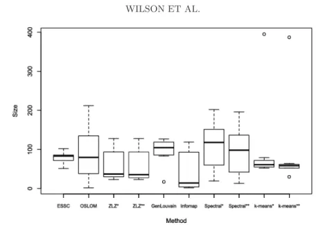
We note that the ZLZ,k-means and Spectral methods require prior spec-ification of the number of discovered communities. Based on the ESSC and GenLouvain results, we ran each of these methods with seven and eight detected communities. We show the size distributions of the detected com-munities for each method in Figure4, and find that the size distribution is broadly similar across the ESSC, ZLZ, GenLouvain and Spectral methods. Infomap found many (NC = 18) small communities, including several com-munities of size three or fewer. At both k= 7 and 8, k-means found one large community as well as many small similarly sized communities.

Inter-Table 4

A summary of the detection methods run on the Caltech Facebook network. From left to right,NC is the number of communities detected,S is the average size of the

communities,σˆS is the standard deviation of the community size,Mis the average

number of communities to which nonbackground vertices belong,Dsig is the average

degree of the vertices in a community, DB is the average degree of the background

vertices,PB is the proportion of background vertices, and Eˆ is the mean classification

error associated with the dormitory feature of the individuals. *Methods were set to find 7 and 8 communities, based on the number of communities detected by ESSC and

GenLouvain. —: represents repeated values

Method NC S σˆS M Dsig DB PB Eˆ ESSC 7 78.57 16.03 1.034 55.75 15.81 0.3018 0.0925 OSLOM 18 86.78 63.25 1.085 50.30 6.18 0.1496 0.2011 ZLZ* 7 62.14 41.97 1 64.08 16.60 0.4291 0.5346 ZLZ* 8 58 40.58 – 62.44 14.53 0.3911 0.5323 GenLouvain 8 95.25 35.75 – 43.70 NA NA 0.2576 Infomap 18 42.33 46.23 – – – – 0.8132 Spectral* 7 108.86 72.77 – – – – 0.4865 Spectral* 8 95.25 61.52 – – – – 0.4512 k-means* 7 108.86 126.51 – – – – 0.4242 k-means* 8 95.25 118.35 – – – – 0.4327

Fig. 4. The size distributions of communities from each detection method when run on the Caltech network.

estingly, GenLouvain also produced an eighth community of size twenty-one, all of whose vertices were part of the background vertex set determined by ESSC. No method found significant overlap among the detected commu-nities. The average number of communities to which each vertex belonged ranged from 1 to 1.085. Each of the methods capable of detecting back-ground (ESSC, OSLOM and ZLZ) designated more than 15% of the total network as background, and vertices contained within communities had av-erage degree nearly three times that of background vertices. This suggests, as expected, that the background vertices are less connected to other vertices in the network.

4.1.2. Community features. One motivation for community detection

methods is their ability to find communities of vertices that represent inter-esting, but possibly unavailable, features of the system under study. Here, we explore the ability of each method to capture the demographic features of the Caltech network. To do this, we measure the extent to which the demographic features “cluster” within communities. Typical pair counting measures do not work well here, as the detected communities may overlap and may not cover the entire network. Also, pair counting measures treat the features as a “ground truth” partition of the network, whereas the true structure of a network is often more complex [Yang and Leskovec (2012), Lee and Cunningham (2013)]. As an alternative, we address the connection between communities and features through the problem of classification [see, e.g., Shabalin et al. (2009), Hastie, Tibshirani and Friedman (2001)]: for each

vertex, we treat its community identification as a predictor and its demo-graphic features as a discrete response that we wish to predict. We describe our approach in more detail.

Suppose that a detection method divides the vertices of the network into

K communities plus background. Then the n×K matrix X = [xi,j] de-fined by

xi,j=

1, if vertexi belongs to communityj,

0, otherwise,

represents the detected community structure of the network. For a given demographic feature α taking L-values, let yα

i ∈[L] be the value of α in samplei. We ignore samples for which the value of featureαis not available. Treating the ith row of the matrix X as a K-variate predictor for yα

i , we use the Adaboost classification method [Freund and Schapire (1997)] with tree classifiers to construct a prediction ruleφ:{0,1}K_→[L].

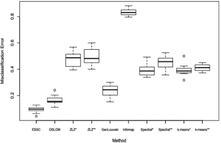
To evaluate each method, we first randomly divide thensamples into ten equally sized subgroups. Then by setting aside one subgroup as a test set, we train the classifier on the remaining subgroups and predict the features of the test set. By subsequently treating each subgroup as a test set in this way, we calculate the misclassification error associated with each test. We report the average misclassification error ˆE for each method as a means of comparison and report the results in Table 4. The distribution of errors is shown in Figure5. Values of ˆE near zero suggest that the detected

commu-Fig. 5. The misclassification error of each method based on the ten-fold classification study performed on the Caltech network. The community containment of each individual was used to classify his/her dormitory residence. For each test, an Adaboost classifier was used for comparison.

nity structure captures the clustering of the selected feature. We consider the dormitory residence of the network, as this feature has been shown to be most representative of the community structure in past studies [Traud, Mucha and Porter (2012)]. From Figure5, we see that ESSC has the lowest misclassification error among competing methods in this classification study. These results suggest that the detected communities of ESSC best match the dormitory residence of the Caltech network.

4.2. Political blog network. The political blog network of Adamic and Glance (2005) represents the hyperlink structure of 1222 political blogs in 2005 near the time of the 2004 U.S. election. Undirected edges connect two blogs that have at least one hyperlink between them. The blogs were pre-classified according to political affiliation by the authors in Adamic and Glance (2005). These authors, as well as those of Newman (2006), observed that blogs of a similar political affiliation tend to link to one another much more often than to blogs of the opposite affiliation. We show a force directed layout of this network colored by political affiliation in Figure3(B).

4.2.1. Quantitative comparison. We first compare the communities de-tected by each method based on their quantitative characteristics. The re-sults are summarized in Table 5. ESSC took 2.012 seconds to run on this network.

Both the ESSC algorithm and GenLouvain found two large communities of similar size. Interestingly, Infomap found six communities, thirty-four of which contained fewer than 25 vertices. Roughly 95% of the vertices in these smaller communities of Infomap were contained in the background ver-tices of ESSC. Neither ESSC nor OSLOM found significant overlap among

Table 5

A summary of the detection methods run on the Political blog network. The statistics shown here are the same as those in Table 4. *We setkto 2 to match the results of GenLouvain and ESSC. **We chosek as 10 so that at least 50 percent of the vertices

were placed in a community

Method NC S σˆS M Dsig DB PB Eˆ ESSC 2 448.50 75.66 1 36.322 2.577 0.2651 0.0201 OSLOM 11 87.58 79.48 1.110 33.749 5.342 0.225 0.0306 ZLZ** 10 60.00 37.69 1 35.50 2.50 0.506 0.1341 GenLouvain 2 611.00 72.12 – 27.36 NA 0 0.0475 Infomap 36 33.94 125.74 – – – – 0.0532 Spectral* 2 611.00 858.43 – – – – 0.3821 k-means* 2 611.00 613.77 – – – – 0.2856

the communities, reflecting the tendency of the political bloggers to com-municate with like-minded individuals: as noted by the authors of Adamic and Glance (2005), “divided they blog.”

ESSC, OSLOM and ZLZ each assigned over twenty percent of the ver-tices to background. The pairwise Jaccard score of these background sets is greater than 0.67 in each case. The background vertices of all three extrac-tion methods had mean degree six times smaller than vertices within com-munities, suggesting the presence of sparsely connected background vertices in this network.

4.2.2. Political affiliation. We now evaluate the extent to which the po-litical affiliation of the blogs “cluster” by conducting the same classification study detailed in Section 4.1.2. We report the mean proportion of misclas-sified labels ˆE in Table 5. ESSC, OSLOM, GenLouvain and Infomap all maintained classification errors below 10%, suggesting that political affili-ation is captured by the network’s community structure quite well. ESSC had the lowest misclassification error in this study, keeping an error be-low 4% across all tests. We look deeper into the strength of connection of the background vertices to the true political affiliations. Interestingly, these vertices were still preferentially attached to their true affiliation, however, their associated p-values were typically greater than 0.10, indicating weak affiliation.

4.3. Personal Facebook network. The personal Facebook network gives friendship structure of the first author’s friends on Facebook. In addition, each individual is labeled according to the time period during which he or she met the first author. This data set, as well as the labels, is provided in the supplemental file [Wilson (2014)]. This network is shown, colored by label, in Figure3(C).

The understanding of human social interactions has been improved through the analysis of large available social networks like Facebook [Lee and Cun-ningham (2013), Traud et al. (2011), Traud, Mucha and Porter (2012)]. Typically, these networks capture the social activity of individuals of a sin-gle location. For example, the Facebook network analyzed in Section 4.1 reflects the friendships of individuals specifically from the California Insti-tute of Technology. The personal Facebook network provides one view of how individuals from different schools and locations interact given that they all have one friend in common.

We ran ESSC on the network (running time about 1 second) and found 7 communities with sizes varying from 10 to 157; see Table6. Approximately 18% of the nodes in the network were distinguished as background. The mean degree of the vertices belonging to a community (Dsig≈33) was about seven

Table 6

Features of the personal Facebook network as well as the results of ESSC. On the left, we list the labels of the individuals according to location and the size of each group. On the right, we list the detected communities and background as well as their corresponding size

True features ESSC results

Label Size Community Size

Acquaintance 80 1 43 A 62 2 107 B 94 3 75 C 150 4 157 D 147 5 53 E 3 6 26 F 3 7 10 G 22 Background 101 (18.0%)

in a community, the average membership was very close to 1, suggesting little overlap between communities.

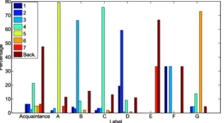
To understand how the location feature of the individuals cluster, we in-vestigate the composition of each label according to detected community in Figure6 and find several interesting results. The individuals from locations A, B, C, D and G all tend to cluster according to the detected communi-ties. For instance, 79% of the individuals from location A were contained in community 5. Similarly, 60% or more of the individuals from locations B, C, D and G also belong to a single community in each case. Groups A, B, C and D represent the schools that the author attended from high school to final graduate school and make up nearly 81% of the total network. Groups

Fig. 6. A bar plot showing the clustering of locations A–G and Acquaintances of the personal Facebook network. For each location label, we show the percentage of individu-als from that location that were contained in each detected community. Communities are labeled 1–7 and Back. represents the background vertices.

E and F are not captured well by the communities, however, this is ex-pected due to the small size of these locations (n= 3 in both cases). Finally, the most highly represented group among the background distinguished by ESSC were acquaintances—individuals met through other friends, events or conferences. These results suggest that friendships in this network cluster are based on location and that the acquaintances of the author are not well connected to his remaining friends.

4.4. Enron email network. The Enron email network from Leskovec et al. (2009) is a large (36,691 vertices), sparse network in which each vertex repre-sents a unique email address. An undirected edge connects any two addresses if at least one email message has been sent from one address to the other. At least one vertex of each edge corresponds to the email address of an employee of the Enron corporation. The network is shown in Figure 3(D). We ran ESSC on the network with α= 0.05. ESSC took approximately 10 minutes to run on this network.

Importantly, the network includes Enron employees as well as advertising agencies and spam sites outside Enron. As such, we expect there to be many background vertices representing spam and advertisement email addresses. On applying ESSC to the network, we indeed find an abundance of back-ground vertices—nearly 83% (30,454 vertices) of the network. The average degree of the vertices within a community is nearly twelve times that of the background vertices. ESSC found 8 communities with average size of 1239 and standard deviation 450. The average membership of the vertices that were contained within a community was 1.409, indicating a moderate amount of overlap of communities.

5. Simulation study. In this section we evaluate the performance of ESSC on simulated networks with three primary types of community structure: (1) communities that partition the network; (2) communities that overlap and cover the network; and (3) disjoint communities plus background.

Networks of the first two types have been well studied, and there are sev-eral existing simulation benchmarks for these structures [Girvan and New-man (2002), Lancichinetti and Fortunato (2009a, 2009b)]. We make use of the Lancichinetti, Fortunato and Radicchi (LFR) benchmark from Lancichinetti and Fortunato (2009a, 2009b) in order to assess the perfor-mance of ESSC and other methods on networks of the first two types. Our principal reason for using the LFR simulation benchmark is its flexibility, as well as the fact that the power-law degree distribution it employs is represen-tative of the degree of heterogeneity present in many real networks [Barab´asi and Albert (1999)]. ESSC performs well on these standard nonoverlapping and overlapping benchmarks, and is in fact competitive with the other detec-tion methods in these settings. We evaluate the results on these benchmarks in the AppendixB.

Relatively little attention has been paid to networks with background vertices, and we are not aware of a simulation benchmark for networks of this sort. We therefore propose a flexible simulation benchmark for networks with background that extends the LFR benchmark, and use it to compare ESSC with competing methods.

In the remainder of the section, we first describe the LFR benchmarks of Lancichinetti and Fortunato (2009a, 2009b) and then show how these benchmarks can be extended to networks with background. We assess the performance of ESSC and other competing methods on networks with back-ground using our proposed benchmark.

5.1. The LFR benchmark. The LFR benchmarks of Lancichinetti and Fortunato (2009a, 2009b) include a number of parameters that govern the community structure of the simulated network; a list is given in Table 7. The edge density of the simulated network is controlled through the size n

of the network and the mean degree D. For example, sparse networks are represented by benchmarks with large nand small D. The degree distribu-tion of simulated networks follows a power law with exponentτ1. Lower and

upper limits of the degree distribution are set to maintain an average degree

Damong vertices in the network. The distribution of community sizes in the LFR benchmark follows a power law with exponentτ2. The size range [s1, s2]

sets lower and upper limits on the size of communities in the network. Con-sider a vertexuand its communityC. Thenushares a fractionµof its edges with vertices outside ofC while the remaining 1−µof its edges are shared with vertices within C. Thus, the mixing parameter µ controls the extent to which communities mix, with communities becoming less distinguishable as µ increases. Finally, in the LFR benchmark with overlap, the parame-ter ρ∈(0,1) is the proportion of vertices that are contained in exactly two

Table 7

Description of the free parameters available with the LFR benchmark networks

Parameter Description

n Size of the network

µ∈₍₀,1) Mixing parameter: the proportion of external community degree for each vertex

τ1 Power-law exponent for degree distribution of network

τ2 Power-law exponent for size distribution of communities in network

D Mean degree

[s1, s2] Size range of each community:s1= lower limit

s2= upper limit

ρ∈(0,1) Proportion of vertices contained in two communities (used in overlapping benchmark only)

communities, and therefore controls the extent of overlap. If u belongs to two communities in the overlapping LFR benchmark, thenµrepresents the proportion of edges ofu that fall outside all these communities.

5.2. Background benchmarks. To assess detection methods on networks with background, we propose three principled test bed simulations: (1) a network with no communities (and therefore all vertices are background); (2) a network with a single embedded community; and (3) a network with disjoint communities and background. In what follows, we first describe how to simulate each type of network and then discuss the results for each type.

Networks with no community structure: It is important to measure the extent to which a detection method correctly identifies the lack of community structure when none is present. We construct such background networks by using two random network models: the Erd˝os–R´enyi model of Erd˝os and R´enyi (1960) where all vertices are linked with equal probability, and the configuration model of Molloy and Reed (1995) where vertices are linked according to a prescribed degree sequence as discussed in Section2.

For each of these models, we vary the sizenand mean degree Din order to control the edge density of the generated network. In particular, for con-figuration random networks, we specify that the degree sequence follows a power law with degreeτ1 and average degree D.

Single embedded community: We consider networks that contain a single embedded community and many background vertices. To construct such networks, we use a variant of the stochastic two block model of Snijders and Nowicki (1997), that has a simple generative procedure. First, vertices are placed randomly and independently in two blocks,C1 and C2, according to

the probabilitiesπ1 and π2= 1−π1. An edge is included between a pair of

distinct verticesu∈Ci andv∈Cj with probabilityPi,j, independently from pair to pair.

To construct a network of size n with a single embedded community

C1 and background C2, we generate a stochastic two block model using

π={π,1−π} withπ∈(0,1) and P={P_i,j: 1≤i, j≤2} given by P=θ κ 1 1 1 .

Hereκ >1 controls the inner community edge probability, andθ <1 controls

the average degree of the network. Modifyingπ controls for the size of the embedded community. The parametersθ and ncan be modified to control the edge density of the network. By generating a network of fixed size and mean degree, one can assess the sensitivity of a detection method by running the method across a range ofπ. We note that Zhao, Levina and Zhu (2011) used a similar benchmark network to assess the performance of their own detection algorithm.

Disjoint communities and background: As a third benchmark test set, we simulate a network with background and degree heterogeneities. To do so,

we propose combining the LFR benchmark described in Section 5.1 with

the block structure described above. We construct this network in two steps

using the same parameters as the LFR benchmark described in Table 7.

First, we independently and randomly assign vertices to one of two blocks

C1 andC2according to probabilitiesπ={π,1−π}. We place edges between

vertices in blockC1 according to the disjoint LFR benchmark with

parame-ters Θ = (τ1, τ2, n·π, µ, D·π,[s1, s2]). The remaining vertices, corresponding

to C2, are connected to all vertices with equal probability P2:=D(1−π).

Thus, our benchmark is constructed as a stochastic 2 block model described

by π and P= PLFR P2 P2 P2 ,

where PLFR denotes the edge probabilities between vertices in C1 derived

from the LFR random network. The resulting network has average degreeD. On average, a fractionπ of the vertices exhibit community structure follow-ing the LFR disjoint benchmark, while the remainfollow-ing vertices are connected to each other and to vertices in the first block in an Erd˝os–R´enyi like fashion. This new benchmark is flexible and can be used to assess the performance of any community detection method for networks with background.

5.3. Results. Networks with no community structure: We generated both Erd˝os–R´enyi and configuration model random graphs with 1000 vertices, with average degree D ranging from 10 to 100 in increments of 10. The degree sequence of the vertices in the configuration network follow a power-law distribution with degree τ1= 2. For each value of D, we generate 30

random graphs, with edge probabilities determined by the value of D. In each of the simulations, ESSC assigned all nodes to background, as desired.

Single embedded community: We generated networks of size 2000, and set

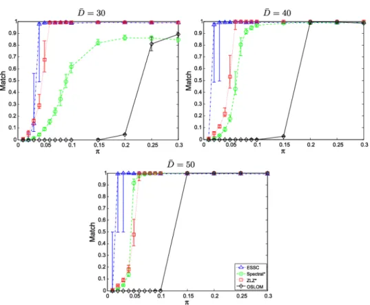
κ to 10, so that the edge probability within the single community is ten times that of the background. We selected values ofθ to generate networks with average degreeD of 30, 40 and 50. For each value of D, we generated networks with embedded communities of size π∗2000 for π ranging from 0.01 to 0.3.

For each set of parameters, we generated 30 network realizations and gave these as input to ESSC, Spectral, ZLZ and OSLOM. We set Spectral to partition the network into two communities and set ZLZ to extract one community, thereby giving both of the methods an advantage over the other methods considered.

In order to measure the ability of each method to find the true single em-bedded community, we used the maximum Jaccard Match score of the de-tected communities. In detail, we measured the Jaccard score between each

Fig. 7. The results for networks with a single embedded community. Shown are the first, second and third quartile of the maximum Jaccard Match of each method over 30 realiza-tions across values ofπ. *Spectral and ZLZ were given the true number of communities: Spectral was set to partition the network into two communities, while ZLZ was set to extract 1 community.

detected community and the true embedded community and reported the maximum of these values for each simulation. Results are shown in Figure7. From Figure 7, we see that ESSC is able to find, with Match ≈1, single embedded communities even when the community is as small as 4% of the to-tal network. As the size of embedded community increases, the performance of each method improves, eventually reaching near optimal performance. In the case of small embedded communities (π <0.05), ESSC and ZLZ perform similarly, with ESSC having a slight advantage. Finally, ESSC and all other methods improve as the average degree of the network increases. Across all simulations, we note that OSLOM did not find more than two nontrivial communities.

Disjoint communities and background: We simulated networks of size n= 2000 with π= 1/2, so that half of the vertices were background and the other half belonged to disjoint communities generated according to the LFR

benchmark. Networks were generated with average degreeD= 30, 40 and 50, with community sizes in the range [s1, s2] = [20,100]. Degree distributions

were generated according to a power law with degree exponentτ1= 2 and

community size distributions were generated according to a power law with degree exponentτ2= 1. For each value of D, networks were generated with

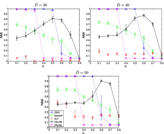
mixing parameter µ ranging between 0.1 and 0.8 in increments of 0.1. For each set of parameters 30 network realizations were generated and then passed as input to ESSC, Spectral, ZLZ, OSLOM and Infomap. As before, the Spectral and ZLZ were run using the true number of communities. The generalized normalized mutual information (NMI) was used to measure the concordance of the detected communities and the true communities with background vertices treated as a single community. NMI is an information theoretic tool that can measure the similarity between two partitions as well as between two covers of a network. For more information on this similarity measure, refer to Lancichinetti, Fortunato and Kert´esz (2009). Results are shown in Figure8.

Figure8tells us several interesting things about the performance of ESSC and other detection methods on complex networks with background. First, we see that ESSC performs well (NMI≈1) across a range of mixing param-etersµfrom 0.1 to 0.5. Afterµ= 0.6, ESSC finds no significant communities and, hence, the performance falls at this point. Infomap competes favorably with ESSC up untilµ= 0.3, at which point Infomap places all vertices in the same community. Interestingly, OSLOM has a peak of performance around

µ= 0.6. This appears to hinge on the fact that the method measures the strength of a community through assuming that vertices outside a commu-nity are close to the connectivity of the vertex of the commucommu-nity that has the lowest connectivity for the specified community. Highly mixed commu-nities tend to favor this similarity, giving OSLOM an advantage in these cases. Importantly, ESSC performs nearly as well on networks of disjoint communitieswith background vertices as it does on these types of networks

without background (see the AppendixB for nonbackground simulations). On the other hand, the remaining methods tend to, on average, perform much worse when background vertices are introduced.

6. Discussion. The identification of communities of tightly connected vertices in networks has proven to be an important tool in the exploratory analysis and study of a variety of complex connected systems. In this paper we introduced a means to measure the statistical significance of connection between a single vertex and any collection of vertices in undirected networks through a reference distribution derived from the properties of the condi-tional configuration model. We introduced and evaluated a testing based community detection method, ESSC, which identifies statistically signifi-cant communities through the use of p-values derived from this reference

Fig. 8. The results for networks with LFR and background features. Shown are the first, second and third quartile match of each method over 30 realizations across values of µ. The degree distribution of the significant community structure follows a power law with exponent τ1= 2with average degree D specified in each figure. *Here, Spectral and ZLZ

were given the true number of communities.

distribution. This method automatically chooses the number of communi-ties and relies only upon one parameter which guides the false discovery rate of discovered communities.

The ESSC extraction technique directly addresses the importance of iden-tifying background vertices within a network that need not necessarily be assigned to identified communities. Given the heterogeneities of vertex roles in most real-world network data, identifying background nodes is an im-portant aspect of community detection. Methods which identify background vertices can help prevent the noise associated with their connections from polluting the otherwise significant features among and between communi-ties.

We evaluated ESSC and a number of competing community detection methods using a variety of quantitative and network-specific validation mea-sures. We have shown that ESSC is able to capture features of network data

that are relevant to the modeled complex system. For instance, in the Caltech network study we found that ESSC identified communities closely match-ing the dormitory residence of its individuals; similarly, in the political blog study ESSC identified communities matching the political affiliation of the bloggers in the network. Importantly, ESSC identified a moderate amount of background for each analyzed network in this paper, suggesting potential benefits to distinguishing background in a network.

Finally, through a series of simulations we have shown that ESSC is able to successfully capture both overlapping and disjoint community structure, as well as community structure in networks with background. In the former scenario, ESSC is competitive with many modern detection methods, while in the latter we find that ESSC outperforms competing methods.

The development of ESSC relied on undirected, unweighted networks, however, this can be extended to networks of different structures, including directed, multilayer and time-varying networks. Understanding the statisti-cal significance of communities in each of these more complex network struc-tures requires both theoretical and methodological work, providing avenues for future research. This includes comparing ESSC to the various stochas-tic block model fitting algorithms and other permutation-based statisstochas-tical methods that have been recently developed over the past few years. Fur-thermore, understanding the consistency properties of the ESSC algorithm is an interesting question of independent interest which will require recently developed probabilistic tools.

APPENDIX A: APPROXIMATE DISTRIBUTION OF ˆD(U:B)

Here we state and prove Theorem 1 which gives the approximate law of ˆ

dn(u:B) on which our algorithm is based in the large network limit. The result is specific to the conditional configuration model, which we use as a null network model in order to find significant community structure.

Proof of Theorem1. Equation (2.2) implies that for the number of edges Eo,n one has

Z R x dFn(x) = ∞ X k=0 kNk(n) n = 2 |Eo,n| n ∼µ,

whereNk(n) is the number of vertices of degree k. Thus,|Eo,n| ∼nµ/2. Now to understand the distribution of ˆdn(u:B), namely, the number of connections of vertexuto the subsetB in CM(do,n), we use the fact that for constructing the configuration model, one can start at any vertex and start sequentially attaching the half-edges of that vertex at random to available