(will be inserted by the editor)
Mohamed F. Mokbel · Walid G. Aref
SOLE: Scalable On-Line Execution of Continuous Queries
on Spatio-temporal Data Streams
the date of receipt and acceptance should be inserted later
Abstract This paper presents the Scalable On-Line Execution algorithm (SOLE, for short) for continuous and on-line evaluation of concurrent continuous temporal queries over data streams. Incoming spatio-temporal data streams are processed in-memory against a set of outstanding continuous queries. The SOLE algo-rithm utilizes the scarce memory resource efficiently by keeping track of only the significantobjects. In-memory stored objects are expired (i.e., dropped) from memory once they becomeinsignificant. SOLE is a scalable algo-rithm where all the continuous outstanding queries share the same buffer pool. In addition, SOLE is presented as a spatio-temporal join between two input streams, a stream of spatio-temporal objects and a stream of spatio-temporal queries. To cope with intervals of high arrival rates of objects and/or queries, SOLE utilizes a load-sheddingapproach where some of the stored objects are dropped from memory. SOLE is implemented as a pipelined query operator that can be combined with tra-ditional query operators in a query execution plan to sup-port a wide variety of continuous queries. Performance experiments based on a real implementation of SOLE in-side a prototype of a data stream management system show the scalability and efficiency of SOLE in highly dy-namic environments.
This work was supported in part by the National Sci-ence Foundation under Grants IIS-0093116, IIS-0209120, and 0010044-CCR.
Mohamed F. Mokbel
Department of Computer Science and Engineering, Univer-sity of Minnesota, Minneapolis, MN, 55455 E-mail: [email protected]
Walid G. Aref
Department of Computer Science, Purdue University, West Lafayette, IN 47907 E-mail: [email protected]
1 Introduction
The wide spread of location-detection devices (e.g., GPS devices, handheld devices, and cellular phones) results in new environments where massive spatio-temporal data are continuously streamed out from mobile users. The high arrival rates of spatio-temporaldata streamsalong with its massive data sizes make it infeasible for tradi-tional spatio-temporal data management techniques to store, query, or index incoming spatio-temporal data. Unfortunately, most of the exiting techniques for spatio-temporal databases (e.g., see [27–29,31,33–35,39,43,46, 48,51,52,57]) rely mainly on the basic assumption that all incoming spatio-temporal data can be stored on disk. Thus, continuous query processing techniques (e.g, [27, 39,52,57]) aim to utilize the disk storage to produce in-cremental results of continuous queries. While this as-sumption is valid for certain data sizes and data arrival rates, it may not be feasible for high arrival rates and massive data sizes. When considering data streaming en-vironment, only in-memorysolutions are feasible.
On the other side, recent research efforts in data stream management systems (e.g., see [2,7,13,14,42]) fo-cus mainly on processing continuous queries over tradi-tional data streams. However, the spatial and temporal properties of both data streams and continuous queries are overlooked. Continuous query processing in spatio-temporal streams is distinguished from traditional data streams in the following: (1) Queries as well as data have the ability to continuously change their locations. Thus, spatio-temporal data streams are considered as a series of data updates rather than the append-only model of traditional data streams. (2) An object may be added to or removed from the answer set of a spatio-temporal query. Consider moving vehicles that move in and out of a certain query region. (3) The commonly used model ofsliding-windowqueries [4,5,23] does not support com-mon spatio-temporal queries that are interested on the current state of the database rather than on the recent historical state.
In this paper, we aim to combine the recent advances in both the traditional spatio-temporal query processors and data stream query processors in order to provide an efficient query processing forspatio-temporal streams. Towards this goal, we propose the Scalable On-Line Execution algorithm (SOLE, for short) for continuous and on-line evaluation of concurrent continuous spatio-temporal queries over spatio-spatio-temporal data streams. On-line execution is achieved in SOLE by allowing only in-memory processing of each single data input as it is re-ceived by the system. Such on-line execution model is distinguished from most of the existing spatio-temporal continuous query processors (e.g., [39,46,57]) that buffer a set of updates together and process them once everyT time units.
As in traditional data streaming application, the memory is the most scarce resource. Thus, memory in SOLE is efficiently utilized by keeping track of only those objects that are consideredsignificant. A moving object is consideredsignificant if it satisfies at least one active continuous query. As a result of keeping only those sig-nificantobjects, continuous queries may encounter some regions of uncertainty in which certain moving objects may not be reported in the result. SOLE avoids such query uncertainty regions using a conservative caching approach in which the query area is extended to cover any possible uncertainty area. Scalability in SOLE is achieved by using a shared buffer pool that is accessible by all active queries. Furthermore, SOLE is presented as a spatio-temporal join between two input streams; a streamof spatio-temporal objects and astreamof spatio-temporal queries. To cope with intervals of very high arrival rates of objects and/or queries, SOLE adopts a load-sheddingapproach that dynamically adopts the no-tion ofsignificantobjects based on the current workload. The main goal of load-shedding in SOLE is to support larger numbers of continuous queries, yet with an ap-proximate answer.
The online nature of SOLE makes it possible to en-capsulate its functionalities inside pipelinable query erators that can be combined with traditional query op-erators (e.g., join, aggregates, and distinct) in a query pipeline. Combining traditional query operators with SOLE operators enables the support for a wide variety of complex continuous spatio-temporal queries. In addition, having SOLE as query operators enables the involve-ment of the query optimizer to support multiple can-didate execution plans for continuous spatio-temporal queries. Such design of SOLE results in orders of mag-nitude of performance than traditional spatio-temporal query processing techniques that can be implemented only on-top of existing database engines. The SOLE op-erator is implemented inside the PLACE server [38,40]; a prototype data stream management system for support-ing spatio-temporal applications. In general, the contri-butions of this paper can be summarized as follows:
1. We propose SOLE as the the first attempt to combine spatio-temporal continuous query processing tech-niques with data stream management systems to sup-port continuous queries over spatio-temporal data streams.
2. We show that due to the nature of data stream-ing environments, continuous spatio-temporal queries may encounter uncertainty areas. We show also that SOLE can overcome such uncertainty areas using a conservative caching technique.
3. We provide a scalable framework for SOLE that modifies the commonly used shared execution par-adigm to support data streaming environments, un-certainty areas, and online execution of continuous spatio-temporal queries.
4. We provide load shedding schemes within SOLE that can be triggered at instances of high system work-load. Load shedding techniques aim to support larger numbers of continuous queries with an approximate answer.
5. We encapsulate the functionalities of SOLE into pipelined query operators by utilizing the online na-ture of SOLE. The SOLE operators are implemented inside the PLACE prototype for spatio-temporal data stream management systems.
6. We provide experimental evidence, based on the real implementation of SOLE, that various aspects of SOLE (e.g., query operators, uncertainty manage-ment, scalability, and load shedding) can efficiently support large numbers of continuous queries over spatio-temporal data streams.
The rest of this paper is organized as follows: Sec-tion 2 highlights related work to SOLE in the context of spatio-temporal databases and data stream manage-ment systems. The basic concepts of SOLE are discussed in Section 3. The SOLE algorithms for single and multi-ple continuous spatio-temporal queries are presented in Sections 4 and 5, respectively. Section 6 discusses the load shedding techniques in SOLE. Experimental results that are based on a real implementation of SOLE in-side a data stream management system are presented in Section 7. Finally, Section 8 concludes the paper.
2 Related Work
Up to the authors’ knowledge, SOLE provides the first attempt to furnish query processors in data stream man-agement systems with the required operators and al-gorithms to support a scalable execution of concurrent continuous spatio-temporal queries over spatio-temporal data streams. Since SOLE bridges the areas of spatio-temporal databases and data stream management sys-tems, in this section we discuss the related work in each area separately.
2.1 Spatio-temporal Databases
Existing algorithms for continuous spatio-temporal query processing focus mainly on materializing incom-ing spatio-temporal data in disk-based index structures (e.g., hash tables [12,49], grid files [21,39,44], the B-tree [29], the R-B-tree [33,35], and the TPR-B-tree [48,52]). Thus, it is implicitly assumed that all incoming data can be stored. Scalable execution of continuous spatio-temporal queries is addressed recently for centralized [21, 39,46,57] and distributed environments [9,21]. However, the underlying data structure is either a disk-based grid structure [21,39] or a disk-based R-tree [9,46]. None of these techniques deal with the issue of spatio-temporal data streams where only in-memory solutions are al-lowed. Memory-based data structures have been pro-posed in [31,32,59] to deal with reasonable size of data that can fit in memory, but it is not scalable to large data sizes or streaming environments.
The most related work to SOLE in the context of spatio-temporal databases is the SINA framework [39]. SOLE has common functionalities with SINA where both of them utilize a shared grid structure as a basis for shared execution and incremental evaluation paradigms. However, SOLE distinguishes itself from SINA and other spatio-temporal query processors in the following as-pects: (1) SOLE is an in-memory algorithm where all the employed data structures are built in memory while SINA is a disk-based query processing technique that mainly relies on the disk storage to perform its opera-tions. (2) Due to the size limitations of memory, not all objects are really stored in SOLE. On the other side, in SINA, all data objects are physically stored. (3) As some data objects are not stored, SOLE suffers from having uncertainty areas in its queries where part of the query area may not be aware by the existence of some mov-ing objects. Such scenario cannot happen in SINA as it is proven to be correct based on the knowledge of all stored objects. (4) SOLE is anonlinealgorithm where it produces the incremental result with the change of any location of the query and/or objects. This online feature is in contrast to SINA where SINA buffers all the updates for the lastT time units and processes them as a bulk. Suchonlinebehavior of SOLE makes it suitable to be en-capsulated into a pipelined operator. On the other side, thebulkbehavior of SINA hinders its applicability to be implemented inside real systems. (5) SOLE is equipped with load shedding techniques to cope with intervals of high arrival rates of moving objects and/or queries. The main idea is to drop some data objects from memory to allow for supporting more queries with an approxi-mate answer. Such load shedding cannot be supported in SINA as it is mainly a disk-based algorithm and does not suffer from limited storage space.
2.2 Data Stream Management Systems
Existing prototypes for data stream management sys-tems [1,10,13,15,26,30,42] aim to efficiently support continuous queries over data streams. However, the spa-tial and temporal properties of data streams and/or con-tinuous queries are overlooked by these prototypes. With limited memory resources, existing stream query proces-sors adopt the concept of sliding windows to limit the number of tuples stored in-memory to only the recent tuples [4,5,23]. Such model is not appropriate for many spatio-temporal applications where the focus is on the current status of the database rather than on the recent past. The only work for continuous queries over spatio-temporal streams is the GPAC [37] which is designed to deal only with the execution of a single continuous query.
Scalable execution of continuous queries in tradi-tional data streams aims to either detect common subex-pressions [14,15,36] or share resources at the operator level [4,20,24]. SOLE evaluates multiple spatio-temporal continuous queries as a spatio-temporal join between an object stream and a query stream while a shared memory resource (buffer pool) is maintained to support all contin-uous queries.Load sheddingand adaptive memory man-agement in data stream manman-agement systems are ad-dressed recently in [6,11,18,19,47,53]. The main idea is to either add a special operator to the query plan to regu-late the load by discarding unimportant incoming tuples or dynamically adjust the window size and time granu-larity at runtime. However, none of these approaches can be directly applicable to SOLE as they are not designed to deal with the spatial and temporal properties of data streams. In addition, none of these approaches deals with the special features of SOLE, e.g., uncertainty areas, con-current spatio-temporal queries, and significant objects. Our proposed load shedding techniques are not compet-itive to any of the previous approaches. Instead, they are specifically designed to be applied within the SOLE framework in which previously proposed techniques can-not be applied.
The most related work to SOLE in the context of data stream management systems is the NiagaraCQ frame-work [15]. SOLE has common functionalities with Nia-garaCQ where both of them utilize a shared operator to join a set of objects with a set of queries. However, SOLE distinguishes itself from NiagaraCQ and other data stream management systems in the following: (1) As a result of the spatio-temporal environment, SOLE has to deal with new challenging issues, e.g., moving queries, uncertainty in query areas, incremental evaluation up-dates to the query result. (2) In a highly overloaded sys-tem, SOLE provides approximate results by employing load shedding techniques. (3) In addition to sharing the query operator as in NiagaraCQ, SOLE share memory resources at the operator level.
3 Basic Concepts in SOLE
In this section, we discuss the basic concepts of SOLE including the input/output model, supporting various queries, SOLE pipelined operator, and the SQL syntax.
3.1 Input/Output Model
Input. The inputs to SOLE are two streams: (1) A stream of spatio-temporal data that is sent from continu-ously moving objects with the format (OID, Loc, time), whereOIDis the object identifier, andLocis the current location of the moving object at timetime. For simplic-ity, we consider moving objects as moving pointsin the two-dimensional space. Such scenario depicts the mov-ing of pedestrians, vehicles, or ships in the space. Exten-sions of SOLE to deal with moving regions with various extents and shapes can be done by replacing theLoc at-tribute to be a P olygonattribute with size and shape. In the rest of this paper, we focus on the simple and common case of having moving points. Moving objects are required to send updates of their locations periodi-cally. Failure to do so results in considering the moving object as disconnected. For example, if a movingP did not send any location update in the last t time units, SOLE would delete P from its memory and appropri-ate actions will be taken. (2) A stream of continuous queries. Queries can be sent either from moving objects or from external entities (e.g., a traffic administrator). Although, continuous queries may be be received with different formats, their internal representation at SOLE is unified. In general, a queryQis internally represented as (QID, Region), where QID is the query identifier, andRegionis the spatial area covered byQ. The query region is determined based on the query type. For exam-ple, in range queries, the query region is the area that the query wants to monitor. The rest of this section gives details on how to set the query region.
Output.SOLE employs an incremental evaluation para-digm similar to the one used in SINA [39]. The main idea is to avoid continuous reevaluation of continuous spatio-temporal queries. Instead, SOLE updates the query re-sult by computing and sending only updates of the pre-viously reported answer. This is in contrast to previous continuous query approaches (e.g., [21,34,46,50,51,60, 61]) that abstract the continuous queries to a set of snap-shot queries that are continuously reevaluated with the change of data inputs or queries. SOLE distinguishes be-tween two types of query updates: Positive updatesand negative updates. Apositiveupdate indicates that a tain object needs to be added to the result set of a cer-tain query. In contrast, anegativeupdate indicates that a certain object is no longer in the answer set of a cer-tain query. Thus, the output of SOLE is a stream of tuples with the format (QID,±, OID), where QID is the query identifier that would receive this output tuple,
±indicates whether this output is apositiveornegative update. A positive/negative update indicates the addi-tion/removal of object OID to/from query QID. For example, if a new object P becomes part of the query answer of Q, we send the positive update (Q,+P). On the other side, if an objectP that was in the query an-swer ofQchanges its status to be out of the answer ofQ, we send the negative update (Q,−P) to the query. For more details about the concepts ofpositiveandnegative updates, the reader is referred to [38,39].
3.2 Supporting Various Query Types
SOLE is a unified framework that deals with range queries as well as k-nearest-neighbor (kNN) queries. In addition SOLE supports both stationary and moving queries within the same framework.
Moving Queries. Each moving query is bounded to a focal object. For example, if a moving object M submits a query Q that asks about objects within a certain range of M, then M is considered the focal of Q. A moving query Q is submitted to SOLE as (QID, F ocalID, Region), whereQIDis the query iden-tifier, F ocalID is the object identifier that submits Q, andRegionis the spatial area ofQ. Internally in SOLE, the moving query is represented as (QID, Region) where Regionis a moving area that changes its location accord-ing to the movement of theF ocalID moving object.
kNN Queries. A kNN query is represented as a circular range query. The only difference is that the size of the query range may grow or shrink based on the movement of the query and objects of interest. Ini-tially, a kNN query is submitted to SOLE with the for-mat (QID, center, k) or (QID, F ocalID, k) for station-ary and moving queries, respectively. Internally in SOLE, the kNN query is represented as (QID, Region) where the Region is a circle with center c and radius r. The centercis either stated explicitly ascenterin stationary queries or implicitly as the current location of the object F ocalIDin case of moving queries. Once thekNN query is registered in SOLE, the first incoming k objects are considered as the initial query answer. Then, the radius r is determined as the distance from the query centerc to the kth farthest neighbor. Once the kNN query de-termines its initial circular region, the query execution continues as a regular range query, yet with a variable region size. Whenever a newly coming object P lies in-side the circular query region,Premoves thekth farthest neighbor from the answer set (with a negative update) and adds itself to the answer set (with apositiveupdate). The query circular region isshrunkto reflect the newkth neighbor. Similarly, if an object P, that is one of thek neighbors, updates its location to be outside the circu-lar region, we expand the query circucircu-lar region to reflect the fact that P is considered the farthest kth neighbor. Notice that in case of expanding the query region, we do not output any updates.
3.3 SOLE as a Pipelined Operator
SOLE is encapsulated into a physical pipelined operator that can interact with traditional query operators in a large pipelined query plan. Having the SOLE operator ei-ther in the bottom or in the middle of the query pipeline requires that all the above operators be equipped with special mechanisms to handle negative tuples. Fortu-nately, recent data stream management systems (e.g., Borealis [1], NILE [26], STREAM [42]) have the ability to process such negative tuples.
Basically,negativetuples are processed in traditional operators as follows:SelectionandJoinoperators handle negative tuples in the same way as positive tuples. The only difference is that the output will be in the form of a negative tuple. Aggregates update their aggregate functions by considering the receivednegativetuple. The Distinctoperator reports anegative tuple at the output only if the correspondingpositivetuple is in the recently reported result. For detailed algorithms about handling thenegativetuples in various traditional query operators, the reader is referred to [25].
3.4 SQL Syntax
Since SOLE is implemented as a query operator, we use the following SQL to invoke the processing of SOLE.
SELECT select clause FROMfrom clause WHEREwhere clause INSIDE in clause kNNknn clause
Thein clausemay have one of two forms:
– Static range query (x1, y1, x2, y2), where (x1, y1) and
(x2, y2) represent the top left and bottom right
cor-ners of the rectangular range query. – Moving rectangular range query (′
M′
, ID, xdist, ydist), where ′
M′
is a flag indicates that the query is mov-ing,IDis the identifier of the queryfocalpoint,xdist is the length of the query rectangle, andydistis the width of the query rectangle.
Similarly, theknn clausemay have one of two forms: – Static kNN query (k, x, y), where k is the number of the neighbors to be maintained, and (x, y) is the center of the query point.
– MovingkNN query (′
M′
, k, ID), where ′
M′
is a flag indicates that the query is moving,kis the number of neighbors to be maintained, andID is the identifier of the queryfocalpoint.
4 Execution of Single Continuous Queries in SOLE
To clarify the new ideas used in SOLE, in this section, we present SOLE in the context of single query execu-tion [37]. In the next secexecu-tion, we show how SOLE can be generalized to the case of evaluating multiple concurrent continuous spatio-temporal queries.
4.1 Predicate-based Spatio-temporal Queries
Traditional stream query processing techniques (e.g., see [2,13,42]) employ the so-called sliding-window queriesto accommodate the massive amount of stream-ing data. The main idea is to limit the execution of continuous queries to only the recently received data tuples rather than the whole received tuples. In slid-ing window queries, incomslid-ing streamslid-ing data follow a first-in-first-expire model in which whenever a tuple be-comes old enough, it is expired (i.e., deleted) from mem-ory leaving its space to a more recent tuple. As a re-sult, traditional sliding-window queries can support only (recent) historical queries. Such model is not suitable for temporal queries where most of the spatio-temporal queries in mobile environments are concerned with thecurrent stateof data rather than the recent his-tory.
To suit the needs of mobile environments, SOLE em-ploys a new kind of window queries, termed, predicate-based window queries [22]. In predicate-based window queries, an incoming data tuple is stored in memory only if it satisfies the query predicate. Once an object becomes out of the predicate, it is expired (i.e., deleted) from memory. Thus, data tuples are expired out-of-order. To supportpredicate-basedwindow queries in SOLE, for each queryQ, we store the tuples that satisfyQ’s predi-cate in a data structure termedQ.Answer. Then, if any objectP with locationPoldsends a new location update
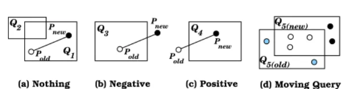
Pnew, SOLE distinguishes among four cases:
– Case I: P ∈Q.Answer and P satisfies Q (e.g., Q1
in Figure 1a). As SOLE reports only the updates of the previously reported result,P will not be sent to the user.
– Case II:P ∈ Q.Answer and P does not satisfyQ (Figure 1b). In this case, SOLE reports a negative updateP−
to the user.
– Case III: P /∈ Q.Answer and P satisfies Q (Fig-ure 1c). In this case, SOLE reports apositiveupdate to the user.
– Case IV:P /∈Q.Answer andP does not satisfyQ (e.g.,Q2 in Figure 1a). In this case,P has no effect
onQ. Thus,P will not be sent to the user.
On the other side, whenever SOLE receives an update from a moving query, it classifies in-memory stored ob-jects into the following four non-overlapped setsC1toC4
P new old Q2 Q1 P old P new new Q3 P old Q4 P 5(new) P Q Q5(old)
(a) Nothing (b) Negative (c) Positive (d) Moving Query Fig. 1 Positive/Negative updates in SOLE.
where: (1)C1is represented by the white objects in
Fig-ure 1d where C1⊂Q.Answer and every moving object
inC1satisfies the newQ.Region. SOLE does not report
any of the objects inC1as none of them affects the
pre-viously reported query result. (2) C2 is represented by
the gray objects in Figure 1d where C2 ⊂ Q.Answer
and none of the objects in C2 satisfies the query
re-gion. For each data object inC2, SOLE produces a
neg-ativeupdate. (3)C3 is represented by the black objects
in Figure 1d where C3 6⊂ Q.Answer and every
mov-ing object in C3 satisfies the new Q.Region. For each
data object in C3, SOLE produces a positive update.
(4)C46⊂Q.Answerand none of the objects inC4
satis-fiesQ.Region(not shown in Figure 1d). SOLE does not produce any output for objects inC4.
4.2 Memory Optimizations
In data streaming environments, storing data objects in disk is not a feasible solution while the memory storage is limited and is considered as the most scarce resource. To efficiently utilize the memory resource, SOLE stores only those data objects that are of interest to the out-standing continuous queries. Considering only a single outstanding continuous queryQ, a moving objectP will be stored in memory only if it satisfies Q. Similarly, if an object P which is stored in-memory becomes out of interest ofQ,P is immediately dropped from memory.
As a general rule, the memory is only occupied by those objects that contribute to the query answer. For example, in Figure 1b, once Pold stepped out form the
query region Q3, it is discarded from memory while in
Figure 1c, Pnew will be stored in memory as it
satis-fies Q4. Similarly, in Figure 1d, all gray objects will be
dropped from memory as they become out of interest of Q5. In this case, the query region is considered as
thepredicatein thepredicate-basedwindow query model where SOLE operates only on those data objects that satisfy the query predicate.
4.3 Uncertainty in SOLE
Since there are many data objects that are not physically stored in SOLE, i.e., those objects that are not of interest to the outstanding query, some uncertainty areas may take place. Theuncertaintyarea of a queryQis defined as follows:
Definition 1 The uncertainty area of query Q is the spatial area ofQthat may contain potential moving ob-jects that satisfyQ, withQnot being aware of the con-tents of this area.
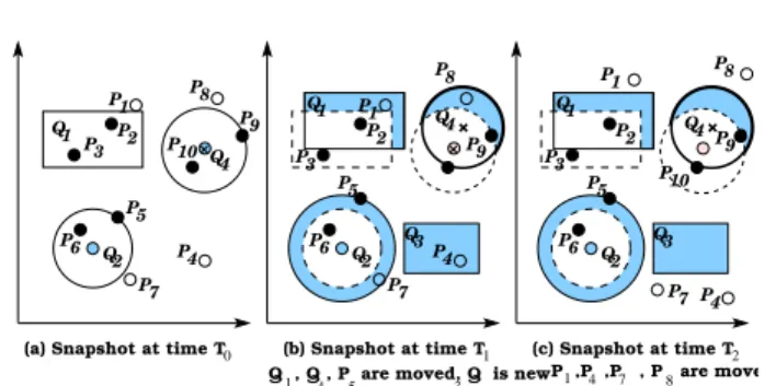
The query uncertainty is a new concept for spatio-temporal data streams. Traditional spatio-spatio-temporal query processing techniques (e.g., SINA [39]) do not suf-fer from any uncertainty as all location data updates are materialized in the disk storage. Thus, traditional spatio-temporal processors provide accurate results which is dif-ferent from the case of SOLE where data are not materi-alized anywhere. In general, SOLE distinguishes among the following three types of uncertainty: uncertainty in new queries, uncertainty in stationary queries, and un-certainty in moving queries. Figure 2 gives an example of these uncertainty types as it represents a three consecu-tive snapshots of a database with ten moving objectsP1
toP10 and four queriesQ1 toQ4.
1. Uncertainty in new queries.Initially, there are no active queries in the system. Thus, continuously ar-rived data streams are neither processed nor stored. Once a queryQis submitted to the system, we can-not provide a fast answer toQ, simply because there is nothing currently stored in the database. In this case, all the area covered byQ is considered an un-certaintyarea. Later on, moving objects update their locations and the answer ofQis progressively built. As an example, consider the moving objectP4in
Fig-ure 2.P4 arrives to the server atT0. Since no query
shows interest in P4 at time T0, P4 is ignored and
not stored in SOLE. Then, at timeT1, a new range
queryQ3is issued. At this time, all the region ofQ3
is considered uncertainty. Since P4 is not stored in
the system, it would not be reported in the query an-swer. At time T2, object P4 sends another location
update to the server, yet, the new location update is outside Q3, thus, it will not be included in the
an-swer. Thus, due to the Q3 uncertainty area,P4 will
not be reported in the query answer though it was in the answer from [T1,T2].
2. Uncertainty in moving queries. Uncertainty in moving queries comes from the fact that those queries tend to cover new spatial areas as they move. New areas may have moving objects that was dropped ear-lier. For example, consider the range queryQ1in
Fig-ure 2. At timeT0(Figure 2a),P1is outside the area of
Q1. Thus,P1is not physically stored in the database.
Recall that only objects that satisfy the query region are stored in the database. At timeT1 (Figure 2b),
Q1 is moved. The shaded area in Q1 represents its
uncertainty area, i.e., the new area covered by Q1.
AlthoughP1is inside the new query region,P1 is not
reported in the query answer where it is not actually stored. AtT2(Figure 2c),P1 moves out of the query
region. Thus,P1is never reported at the query result,
P9 4 P10 P8 P9 Q4
Q , Q , P are moved, Q is new1
5 3 4 P ,P ,P , P are moved1 4 7 8 Q 2 P6 Q1 P3 P5 P7 P2 Q2 P6 P Q1 Q
(a) Snapshot at time T0 Q1 P3 P5 P2 Q2 P6 P7 P1 P2 7 4 Q3 P1 Q4 P9 P8 P10 P8 P P3 P1 P5
(b) Snapshot at time T1 (c) Snapshot at time T2
P4 Q3P4
Fig. 2 Uncertainty in spatio-temporal queries.
interval [T1, T2]. Another example for uncertainty in
moving k−nearest-neighbor (k=2) queries is Q4 in
Figure 2. At time T0 ,P8 is outside the area of Q4.
Thus,P8is not physically stored in the database. At
time T1, Q4is moved. The shaded area inQ4
repre-sents its uncertaintyarea. AlthoughP8 is inside the
new query region,P8is not reported in the query
an-swer where it is not actually stored. AtT2,P8 moves
out of the query region. Thus, P8 is never reported
at the query result, although it was inside the query region in the time interval [T1, T2].
3. Uncertainty in stationary queries. Uncertainty in stationary queries comes from the fact that those queries may change their shapes over time. In this case, new spatial areas that are covered by the new shapes are considered as uncertainty areas. For exam-ple, consider the stationaryk-nearest-neighbor query (k = 2) Q2 in Figure 2. At time T0, the answer of
Q2 is (P5, P6). The query circular region is centered
at Q2 with its radius being the distance from Q2 to
P5. SinceP7 is outside the query spatial region,P7is
not stored in the database. At time T1,P5 is moved
far fromQ2. SinceQ2 is aware only ofP5 andP6, we
extend the region of Q2 to include the new location
of P5. Thus, anuncertaintyarea is produced. Notice
that Q2 is unaware of P7 since P7 is not stored in
the database. At T2, P7 moves out of the new query
region. Thus, P7 never appears as an answer of Q2,
although it should have been part of the answer in the time interval [T1, T2].
In general, the uncertainty area in SOLE comes from the fact that moving objects are not actually stored in the database unless they are needed by existing queries. Such definition of uncertainty is an orthogonal definition from the location uncertainty in moving objects that has been used extensively in the literatures (e.g., [3,16,17,45, 54–56]). Location uncertainty refers to the lower resolu-tion and inaccuracy of locaresolu-tion-detecresolu-tion devices where the system is not aware of the exact location of mov-ing objects. Instead, the system has a vague knowledge about the possible locations of moving objects. In con-trast, in SOLE, the uncertainty is related to the query not to the object as new spatial areas are covered by existing or new queries.
P6 P2 P1 P3 4 P P P7 0 (a) Snapshot at time T
P5 5 1 P2 P P 2 (c) Snapshot at time T P3 P5 P1 P2 P4 1 4 P3 P6 P6 7 P (b) Snapshot at time T All objects are moved
7
The query is moved
P
Fig. 3 Avoiding uncertainty in SOLE (range queries).
4.4 Avoiding Uncertainty in SOLE
SOLE does not handle the uncertainty areas that re-sult from the newly submitted continuous queries. New continuous queries suffer from uncertainty areas for the first few seconds where the query answer is built progres-sively. Continuous queries are issued to run for hours and days. Thus, having awarming upperiod for a few seconds does not affect neither the accuracy nor the efficiency of the query result. Section 7 provides more elaboration on the effect of uncertainty areas of new queries. On the other side,uncertaintyareas that result from stationary or moving queries are crucial and are handled efficiently by SOLE.
SOLE avoids uncertainty areas in moving and sta-tionary spatio-temporal queries using a caching tech-nique. The main idea is to predict the uncertainty area of a continuous queryQ andcache in-memory all mov-ing objects that lie in Q’s uncertainty area. Whenever an uncertainty area is produced, SOLE probes the in-memory cache and produces the result immediately. A conservativeapproach forcachingis to expand the query region in all directions with the maximum possible dis-tance that a moving object can travel between any two consecutive updates. Such conservative approach com-pletely avoids uncertainty areas where it is guaranteed that all objects in the uncertainty area are stored in the cache. The underlying assumption with the conservative cache approach is that all moving objects are required to report their location updates everyttime units. Fail-ure to do so would result in disconnecting the moving object. Theconservativecaching approach requires only the knowledge of the maximum object speed, which is typically available in moving object applications (e.g., moving cars in road network have limited speeds). This is in contrast to all validity region approaches (e.g., the safe region [46], the valid region [60], and the No-Action region [58]) that require the knowledge of the locations of other objects. This information is not available in our case since SOLE is aware only of objects that satisfy the query predicate. Thus, validity region approaches are not applicable in the case of spatio-temporal streams. In the rest of this section, we give two examples of using the conservative caching approach to avoid any uncertainty area in both moving and stationary queries.
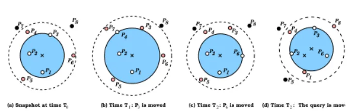
Example 1. Moving Queries. Figure 3 gives an example of usingcachingto avoid uncertainty in moving queries. The shaded area represents the query region.
P 6 2 (c) Time T : P is moved 8 P P 5 P 4 7 P 3 P 6 P 2 1 P 2
(d) Time T : The query is moved 1 P 4 P 3 P 8 P 5 P 7 P 6 P 2 P 1 P 0 (a) Snapshot at time T 8 P 5 P 2 P 1 P 3 P 7 P 6 P 4 P 3 1 (b) Time T : P is moved 8 P 7 P P 4 6 P P 5 P 2 P 3
Fig. 4 Avoiding uncertainty in SOLE (kNN queries).
The cached area is represented as a dashed rectangle. Moving objects that belong to the query answer or to the query’s cache area are plotted as white or gray cir-cles, respectively. At time T0 (Figure 3a), two objects
satisfy the query answer (P1, P2), three objects are in the
cache area (P3, P4, P5), and two objects outside the cache
area (P6, P7). Only objects that either in the query or
the cache area are stored in-memory. AtT1 (Figure 3b),
all objects change their locations. However, we only re-portP−
2 and P
+
3 . The cache area is updated to contain
(P2, P4, P6). Changes in the cache area do NOT result
in any updates. At T2 (Figure 3c), the query Q moves
within its cache area. Two updates are sent to the user; P−
3 and P
+
4 . The cache area is adjusted to contain P3
and P6 only. Notice that without employing the cache
area, we would miss P+ 4 .
Example 2. Stationary Queries.Figure 4 gives an example of continuousk-nearest-neighbor query (k= 3). A snapshot of the database at time T0 is given in
Fig-ure 4a with P1, P2, andP3 represent the query answer.
P4,P5, andP6are stored in the cache list, whileP7and
P8 are not stored in the database (since they are
out-side the cache region). At timeT1(Figure 4b), objectP3
moves out of the query region but not outside the cached area. SinceP3 is still inside thecachearea, we probe the
cachelist to findP4that is nearer to the focal point than
P3. Thus, we send a negativeupdate P −
3 and a positive
updateP4+ to indicate that the current answer contains
P1, P2, and P4. At timeT2 (Figure 4c),P6 moves from
the cache area into the query area. Thus,P6is nearer to
the query focal point than thekth previous answer (P4).
Thus, we send the negativeupdate P−
4 and the positive
updateP+
6 to indicate that the current answer contains
P1, P2, and P6. At time T3 (Figure 4d), the query is
moved along with its cache area. The query movement results in two updates: thenegative updateP−
1 and the
positive updateP3+.
4.5 Analysis of the Caching Approach
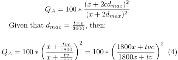
In this section, we study various parameters that affect the performance of the caching technique in terms of both the cache overhead and the query accuracy. With-out loss of generality, we assume that the query original area is a square area with a side lengthx. Also, we as-sume that moving objects are distributed uniformly in the space.
Cache overhead. Assume that the caching tech-nique would increase each side length of the square area by a distanced. Then, the overhead percentage of using thecachingtechnique can be measured by the percentage of the increase in the total area from the original query to the extended query (i.e., the query area plus the cache area). Thus, the cache overhead can be formulated as:
cache overhead= 100×(x+d)
2
−x2
x2
Assuming that the original square side lengthxcan be represented as a factor of the non-zero increase in the side length d, i.e., x = md, where m is termed as the expansion factor of the original query. Then, the cache overhead can be represented as
cache overhead= 100×(md+d) 2 −m2 d2 m2d2 (1) = 100×2md 2+d2 m2d2 = 100× 2m+ 1 m2 (2)
This means that the larger the expansion factorm, the lower the cache overhead. For example, if m is so large, (i.e., order of tens), the cache overhead percentage will be boiled down to be 200
m. Havingmas 50 will result
in only 4% overhead.
To get a better estimation of the value of the ex-pansion factor m and the effect of various paraments, we consider that moving objects have a maximum ve-locity of v miles per hour. Furthermore, moving objects are assumed to report their locations to the server every t seconds, otherwise, moving objects will be considered as disconnected. Thus, the maximum possible distance dmax that a certain moving object can travel between
any two consecutive updates isdmax= 3600t×v. Then, for a
conservative caching approach, we setd= 2dmax to
in-dicate the increase of each query region side by the max-imum possible distance. However, for a non-conservative approach, we only setd= 2×c×dmaxwherec,0≤c≤1,
is a factor that indicates the percentage of caching we would like to have. Having c= 1 indicates the conserva-tive caching approach while having c= 0 indicates that no caching is used. In terms of the velocity v and the time intervalt, the distancedcan be represented as:
d= t×v×c 1800
Since,x=md, the expansion factormcan be repre-sented as:
m= 1800×x
t×v×c (3)
As given in Equation 2, the higher the value ofm, the lower the cache overhead. Then, Equation 3 determines the factors that affect the cache overhead. For example, the higher the value ofx, the original query side length, the lower is the cache overhead percentage. The main
idea is that the larger the original query, the lower the effect of extending its region. Similarly, the lower the value ofc, the higher the value ofm, and hence the lower is the cache overhead. Recall that 0≤c≤1, the lowest value of c would result in a very large value of m. In contrast increasing the value ofvand/ortreducesmand hence increases the cache overhead. This indicates that if moving objects are moving with very high velocity, then it is expected that moving objects would travel relatively long distances between two consecutive updates. Then, the cache area needs to have a large area to accommodate such distance. Similarly, if the time interval t between any two updates is relatively large, then the distance between two consecutive updates would call for a large cache area and hence a large percentage of the cache overhead.
Query accuracy. The conservative cashing ap-proach guarantees to have 100% query accuracy as all uncertainty areas are covered, i.e.,c= 1. Thus, the query accuracy QA is measured as the ratio of the extended
query area with respect to the area covered by the con-servativeapproach:
QA= 100∗
(x+ 2cdmax)2
(x+ 2dmax)2
Given thatdmax= t
×v 3600, then: QA= 100∗ x+ tvc 1800 x+ tv 1800 2 = 100∗ 1800x+tvc 1800x+tv 2 (4) Example. In a practical scenario, consider a square range query with side lengthx= 3 miles that monitors the traffic in a downtown area. If objects are moving with speedv= 30 miles/hour while updating their loca-tions everyt= 30 seconds, then the maximum traveled distance for each object isdmax= 1/4 mile. Using a
con-servativecaching approach, i.e.,c= 1, then the increase in the side length is d = 1/2 mile. Thus, the expan-sion factorm= 6, and the percentage of the increase in the query area is only around 35% (from Equation 2). On the other hand, because c = 1, then the query ac-curacy is 100% (from Equation 4). However, if we use a non-conservative caching withc= 0.5, then, d= 1/4, m= 12, and the cache overhead will be only 17% (Equa-tion 2), while the query accuracy will be dropped to 86% (Equation 4). Similarly, ifc = 0.25, the cache overhead will be only 8.5% while the query accuracy is 80%. Fi-nally, in the extreme case, i.e., when c = 0, there is no cache overhead at all. In this case, as computed from Equation 4, the query accuracy drops to 73%.
5 SOLE: Scalable On-Line Execution of Continuous Queries
In a typical spatio-temporal application (e.g., location-based servers), there are large numbers of concurrent
spatio-temporal continuous queries. Dealing with each query as a separate entity (e.g., as discussed in Section 4) would easily consume the system resources and degrade the system performance. In this section, we present the scalability of SOLE in terms of handling large numbers of concurrent continuous queries of mixed types (e.g., range and kNN queries). Similar to the SINA frame-work [39], SOLE employs bothshared executionand in-cremental evaluation paradigms as a means to achieve scalability. However, SOLE employs these paradigms in a completely different environments that include, data streaming, in-memory only algorithms and data struc-tures, online execution where the query answer is imme-diately updated with any change in the input. Without loss of generality, all the discussion in the rest of this pa-per is presented in the context of stationary and moving range queries. The applicability to k-nearest-neighbor queries is straightforward as described in Section 3, Fig-ure 2, and FigFig-ure 4. Basically, ankNN query is treated as range queries, yet with only a variable region size.
5.1 Overview of Sharing in SOLE
Figure 5a gives the pipelined execution ofN queries (Q1
toQN) of various types with no sharing, i.e., each query
is considered a separate entity. The input data stream goes through each spatio-temporal query operator sepa-rately. With each operator, we keep track of a separate buffer that contains all the objects that are needed by this query (e.g., objects that are inside the query region or its cache area). With a separate buffer for each sin-gle query, the memory can be exhausted with a small number of continuous queries.
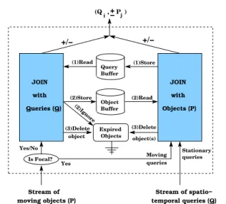
Figure 5b gives the pipelined execution of the same N queries as in Figure 5a, yet with the shared SOLE operator. The problem of evaluating concurrent continu-ous queries is reduced to a spatio-temporal join between two streams; a stream of moving objects and a stream of continuous spatio-temporal queries. The shared spatio-temporal join operator has a shared buffer pool that is accessible by all continuous queries. The output of the sharedSOLE operator has the form (Qi,±Pj) which
in-dicates an addition or removal of objectPjto/from query
Qi. The shared SOLE operator is followed by asplit
op-erator that distributes the output of SOLE either to the users or to the various query operators. The split oper-ator is similar to the one used in NiagaraCQ [15] and it is out of the focus of this paper. Our focus is in realiz-ing: (1) The shared memory buffer, and (2) The shared SOLE spatio-temporal join operator.
5.2 Shared Memory Buffer
SOLE maintains a simple grid structure that divides the space into equal non-overlapped rectangular cells as
Q1 Q2 QN . . Range . . +/− . . Q1 Q2 QN Split +/− +/− Queries (Q) Objects (P)
Stream of Moving Objects (P) +/− +/−
+/−
buffer for each query (a) Separate query plan and
buffer pool for all queries (b) Shared operator and shared
+ − j i (Q , P ) Stream of Spatio−temporal Moving Stream of Buffer . . . Operator Range . . . . . . kNN . . . . . . Join Shared Spatio−temporal
Fig. 5 Overview of shared execution in SOLE.
an in-memory shared buffer pool among all continuous queries and objects. The shared buffer pool is logically divided into two parts; aquery bufferthat stores all out-standing continuous queries and anobject buffer that is concerned with moving objects. In addition to the grid structure, SOLE employs a hash tablehto index moving objects based on their identifers. To optimize the scarce memory resource, SOLE employs two main techniques: (1) Rather than redundantly storing a moving objectP multiple times with each queryQi that needs P, SOLE
storesP at most once along with a reference counter that indicates the number of continuous queries that needP. (2) Rather than storing all moving objects, SOLE keeps track with only thesignificantobjects. Insignificant ob-jects are ignored (i.e., dropped) from memory.Significant objects are defined as follows:
Definition 2 A moving object P is considered signif-icant if P satisfies any of the following two conditions: (1) There is at least one active continuous queryQthat shows interest in objectP (i.e.,P has a non-zero ref-erence counter), (2)P is the focal object of at least one active continuous query.
We define when a query Q shows interest in an objectP as follows:
Definition 3 A query Qis interested in objectP if P either lies inQ’s spatial area or inQ’s cache area.
Having the previous definition of significantobjects, SOLE continuously maintains the following assertion: Assertion 1 Only significant objects are stored in the shared memory buffer
To always satisfy this assertion, SOLE continuously keeps track of the following: (1) A newly incoming data objectPis stored in memory only ifPissignificant, (2) If an object P that is already stored in the shared buffer becomes insignificant, we dropP immediately from the shared buffer. Significant moving objects are hashed to grid cells based on their spatial locations. An entry of a significant moving object P in a grid cell C has the
Buffer Object Expired Objects (1)Read (3)Delete object(s) (2)Ignore queries Stationary queries + − j i (Q , P ) (1)Store with Moving object (3)Delete temporal queries (Q) moving objects (P) Queries (Q) Objects (P) with JOIN +/− +/− Yes/No Yes (2)Read JOIN Stream of spatio− Stream of Query Buffer Is Focal? (2)Store
Fig. 6 Shared join operator in SOLE.
form (PID, Location,RefCount,FocalList). PID and Lo-cationare the object identifer and location, respectively. RefCountindicates the number of queries that are inter-ested inP. FocalListis the list ofactivemoving queries that have P as their focal object. Unlike data objects that are stored in only one grid cell, continuous queries are stored in all grid cells that overlap either the query spatial area or the query cache area. A query entry in a grid cell contains only the query identifier (QID). The spatial region for each query is stored separately in a global lookup table in the format (QID, Region).
5.3 Shared Spatio-temporal Join Operator
Overview. Figure 6 puts a magnifying glass over the shared spatio-temporal join operator in Figure 5b. For any incoming data object, say P, the shared spatio-temporal join operator consults its query buffer to check if any query is affected by P (either in a positive or a negative way). Based on the result, we decide either to storeP in the object buffer or to ignorePand deleteP’s old location (if any) from the object buffer. On the other hand, for any incoming continuous query, sayQ, first we storeQor updateQ’s old location (if any) in the query buffer. Then, we consult the object buffer to check if any of the objects needs to be added to or removed fromQ’s answer. Based on this operation, some in-memory stored objects may becomeinsignificant, hence, are deleted im-mediately from the object buffer. Stationary queries are submitted directly to the shared spatio-temporal join operator, while moving queries are generated from the movement of their focal objects.
Algorithm.Based on the data stored in the shared buffer, SOLE distinguishes among four types of data in-puts: (1) A new data objectP that is not stored in mem-ory, (2) Update of the location of object P, (3) A new stationary queryQ, (4) An update of the region of a
mov-Algorithm 1Pseudo code for receiving a new objectP 1: FunctionNewObject(ObjectP,GridCellCP)
2: foreach QueryQi∈CP ANDP∈Qˆi do
3: P.Ref Count+ + 4: if (P ∈Qi)then
5: output (Qi,+P).
6: end if
7: end for
8: if P.Ref Count >0then
9: storeP inCP and in hash tableh.
10: end if
(b) Action taken for each case (a) All cases of updating P’s location
L L2 L5 1 L9 4 L3 L P L6 9 3 L4 L7 old +P P +P L8 L2 L1 L L5 L6 L7 L8 L −P IN Out new −P Cache Out Cache RefCount−− RefCount−− RefCount++ RefCount++ IN
Fig. 7 All cases of updatingP’s location.
ing query Q. Algorithms 1, 2, 3, and 4 give the pseudo code of SOLE upon receiving each input type. The de-tails of the algorithms are described below. SOLE makes use of the following notations: ˆQindicates the extended query region that covers the cache area so thatQ⊂Q.ˆ CQ, ˆCQ are the set of grid cells that are covered by Q
and ˆQ, respectively.CP represents a single grid cell that
covers the objectP.
Input Type I: A new objectP. Algorithm 1 gives the pseudo code of SOLE upon receiving a new object P in the grid cellCP (i.e., P is not stored in memory).
P is tested against all the queries that are stored inCP
(Lines 2 to 7 in Algorithm 1). For each query Qi ∈CP,
only three cases can take place: (1) P lies in ˆQi but
not in Q. In this case, we need only to increase the ref-erence counter of P to indicate that there is one more query interested in P (Lines 3 in Algorithm 1). Notice that no output is produced in this case sinceP does not satisfy Qi. (2) P satisfies Qi. In this case, in addition
to increasing the reference counter, we output apositive update that indicates the addition of P to the answer set ofQi (Lines 4 to 6 in Algorithm 1). In the above two
cases,P is stored in the shared buffer as it is considered significant. (3)P neither satisfiesQinor lies in ˆQi. Thus,
P is simply ignored as it isinsignificant.
Input Type II: An update ofP.Algorithm 2 gives the pseudo code of SOLE upon receiving an update of ob-jectP’s location. The old location ofP is retrieved from the hash table h. First, we evaluate all moving queries (if any) that have P as their focal object (Lines 2 to 4 in Algorithm 2). Then, we check all the queries that be-long to eitherCP orCPold (Lines 6 to 26 in Algorithm 2) against the line L that connects P and Pold. Figure 7a
gives nine different cases for the intersection ofLwithQ wherePoldandP are plotted as white and black circles,
respectively. BothPoldandP can be in one of the three
Algorithm 2Pseudo code for updatingP’s location. 1: Function UpdateObject(Object Pold,P, GridCell
CPold,CP)
2: foreach queryQi∈P.F ocalListdo
3: UpdateQuery(Qi)
4: end for
5: LetLbe the line (Pold, P)
6: foreach queryQi∈(CPold∪CP)do 7: if QiintersectsLthen 8: if P ∈Qithen 9: Output (Qi,+P) 10: if Pold∈/Qˆi then 11: P.Ref Count+ + 12: end if 13: else 14: Output (Qi,−P) 15: if P /∈Qˆithen 16: P.Ref Count− − 17: end if
18: else if QˆiintersectsLthen
19: if P ∈Qˆithen 20: P.Ref Count+ + 21: else 22: P.Ref Count− − 23: end if 24: end if 25: end if 26: end for
27: if P.Ref Count= 0then
28: deletePoldand ignoreP
29: return.
30: end if
31: if CPold 6=CP then
32: movePold fromCPold toCP. 33: end if
34: Update the location ofPoldto that ofP inCP.
states,in,cache, oroutthat indicates thatP satisfiesQ, in the cache area ofQ, or does not satisfyQ, respectively. The actions taken for each case is given in Figure 7b. Ba-sically, if there is no change of state fromPoldtoP (e.g.,
L1,L5, andL9), no action will be taken. IfPoldwas inQ,
however,P is not (e.g.,L2andL3), we output the
nega-tive update (Q,−P). The reference counter is decreased only whenPoldis of interest toQwhileP is not (e.g.,L3
and L6). Notice that in the case of L2, we do not need
to decrease the reference counter where althoughP does not satisfyQ, P is still of interest toQ asP lies in ˆQi.
Also, in the case ofL6, we do not need to output a
nega-tive update, however we decrease the reference counter. In this case, sinceP and Pold are not in the answer set
of Q, there is no need to update the answer. Similarly, with a symmetric behavior, we output apositiveupdate in the cases of L4 and L7 and we increment the
refer-ence counter in the cases ofL7and L8. After testing all
cases, we check whether objectP becomesinsignificant. If this is the case, we immediately dropP from memory (Lines 27 to 30 in Algorithm 2). IfP is stillsignificant, we update P’s location and cell (if needed) in the grid structure (Lines 31 to 34 in Algorithm 2).
Algorithm 3Pseudo code for receiving a new queryQ. 1: FunctionNewQuery(QueryQ)
2: foreach grid cellcj∈CˆQdo
3: RegisterQincj
4: foreach objectPi∈cj ANDPi∈Qˆdo
5: P.Ref Count+ + 6: if P ∈Qthen 7: output (Q,+P) 8: end if 9: end for 10: end for
Algorithm 4Pseudo code for updatingQ’s location. 1: FunctionUpdateQuery(QueryQold,Q)
2: foreach objectPi∈( ˆCQold∩CˆQ)do 3: if Pi∈Qold then
4: if Pi∈/Qthen
5: Output (Q,−Pi)
6: if Pi∈/Qˆthen
7: Pi.Ref Count− −
8: if Pi.Ref Count= 0then
9: deletePi 10: end if 11: end if 12: end if 13: else if Pi∈Qthen 14: Output (Q,+Pi) 15: if Pi∈/Qˆold then 16: Pi.Ref Count+ + 17: end if
18: else if Pi∈QˆoldANDPi∈/Qˆthen
19: Pi.Ref Count− −,
20: if Pi.Ref Count= 0then
21: deletePi
22: end if
23: else if Pi∈QˆANDPi∈/Qoldˆ then
24: Pi.Ref Count+ +
25: end if
26: end for
27: RegisterQin ˆCQ−CˆQold, 28: unregisterQfrom ˆCQold−CˆQ
Input Type III: A new query Q. Algorithm 3 gives the pseudo code of SOLE upon receiving a contin-uous queryQ. Basically, we registerQin all the grid cells that are covered by ˆQ. In addition, we testQagainst all data objects that are stored in these cells. We increase the reference counter of only those objects that lie in ˆQ. In addition, objects that satisfy Qresults in producing positive updates.
Input Type IV: An update of Q’s region. Algo-rithm 4 gives the pseudo code of SOLE upon receiving an update of a moving query region. The update can be either coming from the user directly or from a change of location of thefocalquery object. Also, the query up-date can be either an upup-date in location or an upup-date in the query area size. All stored objects in all cells that are covered by the old and new regions of Q are tested againstQ. Figure 8a divides the space covered by the old and new regions ofQinto seven regions (R1-R7). The
ac-tions taken for any point that lies in any of these regions
000000000 000000000 000000000 000000000 000000000 000000000 111111111 111111111 111111111 111111111 111111111 111111111 0000000 0000000 0000000 0000000 0000000 0000000 1111111 1111111 1111111 1111111 1111111 1111111 0000000000 0000000000 0000000000 0000000000 0000000000 0000000000 0000000000 0000000000 0000000000 0000000000 0000000000 0000000000 1111111111 1111111111 1111111111 1111111111 1111111111 1111111111 1111111111 1111111111 1111111111 1111111111 1111111111 1111111111 00000 00000 00000 11111 11111 11111 00000 00000 00000 00000 11111 11111 11111 11111
(b) Action taken for each case (a) All cases of updating query region
00000 00000 00000 00000 00000 11111 11111 11111 11111 11111 00000 00000 00000 00000 00000 11111 11111 11111 11111 11111 0000000 0000000 0000000 0000000 0000000 0000000 0000000 0000000 0000000 0000000 1111111 1111111 1111111 1111111 1111111 1111111 1111111 1111111 1111111 1111111 +P RefCount−− Qold Cache +P −P −P IN Out RefCount−− RefCount++ RefCount++ IN Cache Out 1 R2 R4 R5R6 R7 old Q new Q new Q R 3 R R7 R4 R4 R6 R5 R3 R2 R1 R4
Fig. 8 All cases of updatingQ’s region.
are given in Figure 8b. Similar to Figure 7b, a regionRi
could have any of the three statesin,cache, oroutbased on whetherRi is insideQ, is in the cache area ofQ, or is
outsideQ. Basically, no action is taken for objects in any region Ri that maintains its state for bothQ and Qold
(e.g., R4). If a regionRi is insideQold, but is not inQ,
(e.g., R2 andR3), we output anegative update for each
object inRi. We decrement the reference counter of these
objects only if they lie in the region that is out of the new cache area (e.g.,R2) (Lines 3 to 12 in Algorithm 4).
Also, the reference counter is decremented for all objects in the region that are in the old cache area but are out of the new cache area (e.g.,R1) (Lines 13 to 17 in
Algo-rithm 4). Similarly, the reference counter is increased for regionsR6andR7 while apositiveoutput is sent for the
points in regions R5 and R6. Notice that whenever we
decrement the reference counter for any moving object P, we check whetherP becomes insignificant. If this is the case, we immediately dropP from memory (Lines 18 to 25 in Algorithm 4). Finally,Qis registered in all the new cells that are covered by the new region and not the old region. Similarly,Qis unregistered from all cells that are covered by the old region and not the new region.
6 Load Shedding in SOLE
Even with the scalability features of SOLE, the memory resource may be exhausted at intervals of unexpected massive numbers of queries and moving objects (e.g., during rush hours). To cope with such unexpected inter-vals, SOLE employs aload-sheddingapproach that tunes the memory load to support a large number of concur-rent queries, yet with an approximate answer. The main idea is to change the definition ofsignificantobjects (De-finition 2) based on the current workload. By adapting the definition ofsignificantobjects, the memory load will be shed in two ways: (1) In-memory stored objects will be revisited for the new meaning ofsignificantobjects. If an already existing object becomes insignificant accord-ing to the new definition, it is dropped from memory. (2) Newly input data will be tested for significance ac-cording to the new definition. If an object does not meet the new definition of significant objects, it will be ig-nored.
The rest of this section is organized as follows. Sec-tion 6.1 gives a high level architecture of the integraSec-tion
of theload sheddingmodule within the SOLE framework. The accuracy of load shedding is discussed in Section 6.2. Sections 6.3 and 6.4 propose two new methods for re-alizing load shedding inside SOLE, namely, query load shedding and object load shedding. Finally, Section 6.5 discusses maintaining the query accuracy while perform-ing the load sheddperform-ing.
6.1 Architecture of Load Shedding
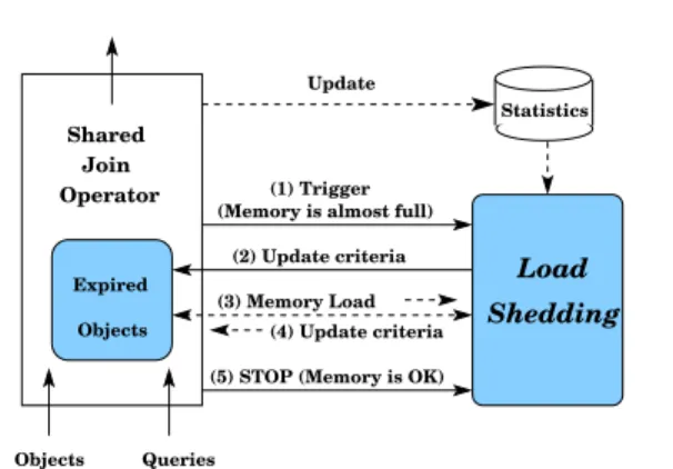
Figure 9 gives the architecture ofload-sheddingin SOLE. Once the shared join operator incurs high resource con-sumption, e.g., the memory becomes almost full, the join operator triggers the execution of theload shedding pro-cedure. The load shedding procedure may consult some statistics that are collected during the course of execu-tion to decide on a new meaning of significant objects. While the shared join operator is running with the new definition of significant objects, it may send updates of the current memory load to theload sheddingprocedure. The load shedding procedure replies back by continu-ously adopting the notion ofsignificantobjects based on the continuously changing memory load. Finally, once the memory load returns to a stable state, the shared join operator retains the original meaning ofsignificant objects and stops the execution of theload shedding pro-cedure. Solid lines in Figure 9 indicate the mandatory steps that should be taken by any load shedding tech-nique. Dashed lines indicate a set of operations that may or may not be employed based on the underlying load sheddingtechnique.
6.2 Accuracy of Load Shedding
Load shedding aims to drop some of the in-memory tu-ples which may be needed by some outstanding queries. As a result, load shedding produces approximate query results. To make sure that the approximate query results are acceptable, whenever a query, say Q, is submitted to SOLE, Qspecifies its minimum acceptable accuracy. Initially, every query Q is evaluated with complete ac-curacy. However, when the system is overloaded,Q’s ac-curacy is degraded to its minimum permissible acac-curacy. Assuming a uniform distribution of moving objects over-all the space, the accuracy of the query answer of SOLE is defined asAccQ= 100×NNActualCurrent whereNCurrentis the
number of stored moving objects within the query range and cache areas while NActual is the number of objects
that should be in both the query range and cache area if load shedding was not employed. Notice that in the case of no load shedding, the query accuracy is 100%. Our definition of the query accuracy is independent from the query type as it relies mainly on the query area. For ex-ample, the accuracy of nearest neighbor queries is com-puted based on the area it covers not on the required number of neighbors.
(3) Memory Load
Queries Objects
(5) STOP (Memory is OK) Update
(1) Trigger (Memory is almost full)
(2) Update criteria (4) Update criteria Statistics Shared Join Operator Expired Objects Shedding Load
Fig. 9 Architecture of load shedding in SOLE.
6.3 Query Load Shedding
The main idea of the query load shedding is to shrink the query area. For example, if it is required to reduce the memory load to only 75%, then we aim to shrink the query area for each single query to its 75%, given that this will be within the permissible query accuracy. Query load shedding is performed in two stages. In the first stage, the query cache area is shrunk. All moving objects that become out of the new query area are elimi-nated if they are not needed by other queries. If the first stage did not result in the desired load shedding, the second stage starts by shrinking the query main area till the minimum permissible accuracy for each query is met or the memory load becomes acceptable. With the query load shedding, all the algorithms given in Section 5 are still valid. The only difference is that the notion of sig-nificantobjects is adopted to be those tuples that lie in thereducedquery area of at least one continuous query. By reducing the query sizes of all continuous queries, objects that are outside the reduced area and are not of interest to any other query are immediately dropped from memory and the corresponding negative updates are sent. During the course of execution, we gradually increase the query size to cope with the memory load. Finally, when the system reaches a stable state, we retain the original query sizes.
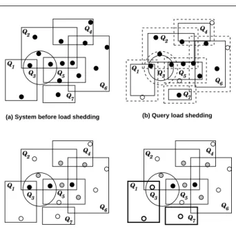
Figures 10a and 10b give an example of query load shedding. The complete snapshot of the database with-out load shedding is given in Figure 10a with seven queries Q1 to Q7 and 15 moving objects. Figure 10b
gives the snapshot of the database after applying the query load shedding. Each query area (including the cache area) is reduced to 90%. This results in dropping a total of four objects (plotted as white circles in Fig-ure 10b) fromQ1,Q4,Q5, andQ6. Given an assumption
of a uniform data distribution over the whole space and the query region, reducing the query area by 10% would result in a 90% query accuracy.
Queryload shedding has two main advantages: (1) It is intuitive and simple to implement where there is no need to maintain any kind of statistical information or