Longitudinal Data Analysis

Longitudinal Data Analysis

Acknowledge: Professor Garrett Fitzmaurice

INSTRUCTOR: Rino

Bellocco

Department of Statistics & Quantitative Methods University of Milano-Bicocca

Department of Medical Epidemiology and Biostatistics

ORGANIZATION OF LECTURES

Longitudinal Data: Basic Concepts Linear Models for Longitudinal Dara

• Modelling the Mean: Analysis of Response Profiles

• Modelling the Mean: Parametric Curves

• Modelling the Covariance

• Linear Mixed Effects Models

LONGITUDINAL DATA ANALYSIS

INTRODUCTION

Longitudinal Studies: Studies in which individuals are measured repeatedly through time.

This course will cover the analysis and interpretation of results from longitudinal studies.

Emphasis will be on model development, use of statistical software, and interpretation of results.

Features of Longitudinal Data

Defining feature: repeated observations on individuals, allowing the direct study of change over time.

Primary goal of a longitudinal study is to characterize the change in response and factors that influence change.

With repeated measures on individuals, one can capture within-individual change.

Note that measurements in a longitudinal study are

Longitudinal data require somewhat more sophisticated

statistical techniques because the repeated observations are usually (positively) correlated.

Sequential nature of the measures implies that certain types of correlation structures are likely to arise.

Correlation must be accounted for in order to obtain valid inferences.

Example 1

Treatment of Lead-Exposed Children (TLC) Trial • Exposure to lead during infancy is associated with

substantial deficits in tests of cognitive ability

• Chelation treatment of children with high lead levels usually requires injections and hospitalization

• A new agent, Succimer, can be given orally

• Randomized trial examining changes in blood lead level during course of treatment

• 100 children randomized to placebo or Succimer

Table 1: Blood lead levels (µg/dL) at baseline, week 1, week 4, and week 6 for 8 randomly selected children.

ID Groupa Baseline Week 1 Week 4 Week 6

046 P 30.8 26.9 25.8 23.8 149 A 26.5 14.8 19.5 21.0 096 A 25.8 23.0 19.1 23.2 064 P 24.7 24.5 22.0 22.5 050 A 20.4 2.8 3.2 9.4 210 A 20.4 5.4 4.5 11.9 082 P 28.6 20.8 19.2 18.4 121 P 33.7 31.6 28.5 25.1 a _{P = Placebo; A = Succimer.}

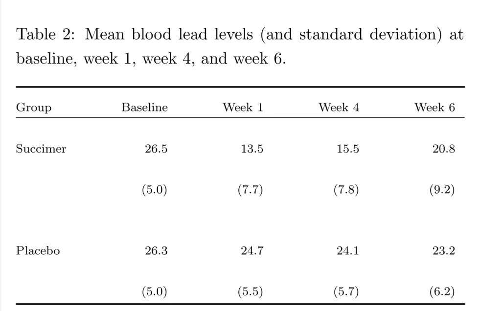
Table 2: Mean blood lead levels (and standard deviation) at baseline, week 1, week 4, and week 6.

Group Baseline Week 1 Week 4 Week 6

Succimer 26.5 13.5 15.5 20.8

(5.0) (7.7) (7.8) (9.2)

Placebo 26.3 24.7 24.1 23.2

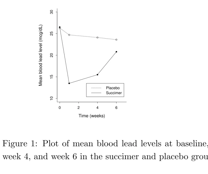
0 2 4 6 10 15 20 25 30 Time (weeks)

Mean blood lead level (mcg/dL)

Placebo Succimer

Figure 1: Plot of mean blood lead levels at baseline, week 1, week 4, and week 6 in the succimer and placebo groups.

Example 2

Six Cities Study of Air Pollution and Health

• Longitudinal study designed to characterize lung function growth in children and adolescents.

• Most children were enrolled between the ages of six and seven and measurements were obtained annually until graduation from high school.

• Focus on a randomly selected subset of the 300 female participants living in Topeka, Kansas.

• Response variable: Volume of air exhaled in the first second of spiromtry manoeuvre, FEV₁.

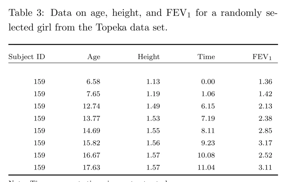
Table 3: Data on age, height, and FEV₁ for a randomly se-lected girl from the Topeka data set.

Subject ID Age Height Time FEV1

159 6.58 1.13 0.00 1.36 159 7.65 1.19 1.06 1.42 159 12.74 1.49 6.15 2.13 159 13.77 1.53 7.19 2.38 159 14.69 1.55 8.11 2.85 159 15.82 1.56 9.23 3.17 159 16.67 1.57 10.08 2.52 159 17.63 1.57 11.04 3.11

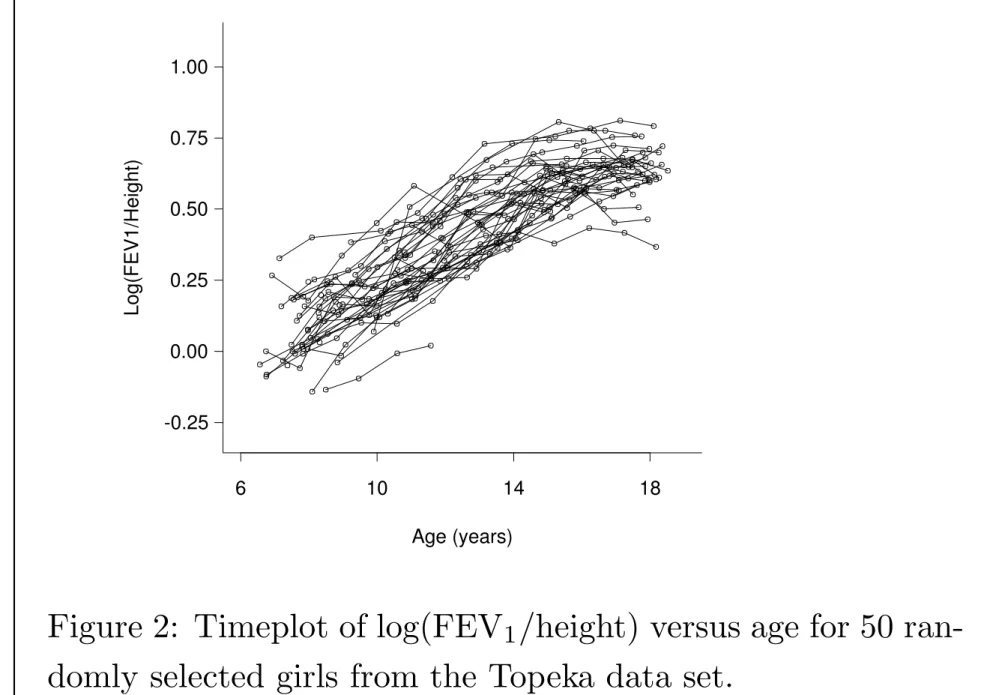
Age (years) Log(FEV1/Height) 6 10 14 18 -0.25 0.00 0.25 0.50 0.75 1.00

Figure 2: Timeplot of log(FEV₁/height) versus age for 50 ran-domly selected girls from the Topeka data set.

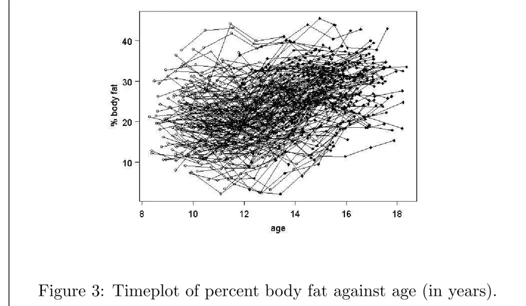
Example 3

Influence of Menarche on Changes in Body Fat

• Prospective study on body fat accretion in a cohort of 162 girls from the MIT Growth and Development Study.

• At start of study, all the girls were pre-menarcheal and non-obese

• All girls were followed over time according to a schedule of annual measurements until four years after menarche.

• The final measurement was scheduled on the fourth anniversary of their reported date of menarche.

• At each examination, a measure of body fatness was obtained based on bioelectric impedance analysis.

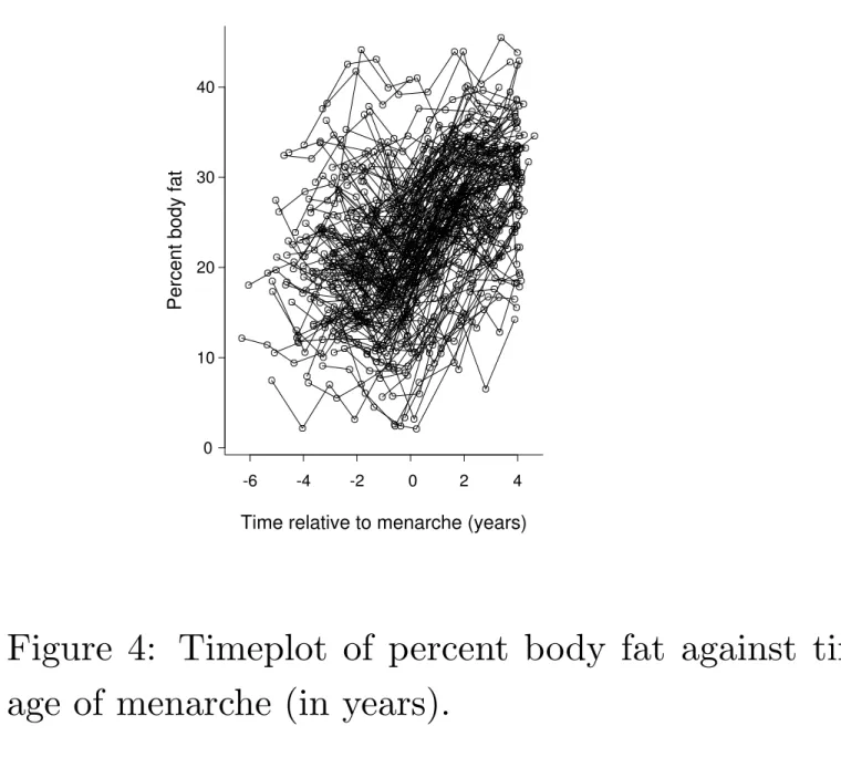
Consider an analysis of the changes in percent body fat before and after menarche.

For the purposes of these analyses “time” is coded as time since menarche and can be positive or negative.

Note: measurement protocol is the same for all girls.

Study design is almost balanced if timing of measurement is defined as time since baseline measurement.

It is inherently unbalanced when timing of measurements is defined as time since a girl experienced menarche.

-6 -4 -2 0 2 4 0 10 20 30 40

Time relative to menarche (years)

Percent body fat

Figure 4: Timeplot of percent body fat against time, relative to age of menarche (in years).

LONGITUDINAL DATA: BASIC CONCEPTS

Longitudinal studies allow direct study of change over time.

The primary goal is to characterize the change in response over time and the factors that influence change.

With repeated measures on individuals, we can capture within-individual change.

A longitudinal study can estimate change with great

precision because each individual acts as his/her own control.

By comparing each individual’s responses at two or more

occasions, a longitudinal analysis can remove extraneous, but unavoidable, sources of variability among individuals.

This eliminates major sources of variability or “noise” from the estimation of within-individual change.

The assessment of within-subject change can only be achieved within a longitudinal study design

In a cross-sectional study, we can only obtain estimates of between-individual differences in the response

A cross-sectional study may allow comparison among

sub-populations that happen to differ in age, but it does not provide any information about how individuals change

In a cross-sectional study the effect of ageing is potentially confounded or mixed-up with possible cohort effects

Terminology

Individuals/Subjects: Participants in a longitudinal study are referred to as individuals or subjects.

Occasions: In a longitudinal study individuals are measured repeatedly at different occasions or times.

The number of repeated observations, and their timing, can vary widely from one longitudinal study to another.

When the number and the timing of the repeated

measurements are the same for all individuals, the study design is said to be “balanced” over time.

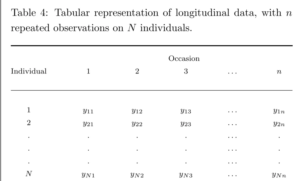
Notation

Let Y_ij denote the response variable for the ith individual (i = 1, ..., N) at the jth occasion (j = 1, ..., n).

If the repeated measures are assumed to be equally-separated in time, this notation will be sufficient.

Later, we refine notation to handle the case where repeated measures are unequally-separated and unbalanced over time. We can represent the n observations on the N individuals in a two-dimensional array, with rows corresponding to individuals and columns corresponding to the responses at each occasion.

Table 4: Tabular representation of longitudinal data, with n

repeated observations on N individuals.

Occasion Individual 1 2 3 . . . n 1 y11 y12 y13 . . . y1n 2 y21 y22 y23 . . . y2n . . . . . . . . . . . . N yN1 yN2 yN3 . . . yN n

Vector Notation:

We can group the n repeated measures on the same individual into a n _× 1 response vector:

Y_i =         Y_i1 Y_i2 .. . Y_in         .

Alternatively, we can denote the response vectors Y_i as

Covariance and Correlation

An aspect of longitudinal data that complicates their

statistical analysis is that repeated measures on the same individual are usually positively correlated.

This violates the fundamental assumption of independence that is the cornerstone of many statistical techniques.

What are the potential consequences of not accounting for correlation among longitudinal data in the analysis?

An additional, although often overlooked, aspect of

longitudinal data that complicates their statistical analysis is heterogeneous variability.

That is, the variability of the outcome at the end of the study is often discernibly different than the variability at the start of the study.

This violates the assumption of homoscedasticity that is the basis for standard linear regression techniques.

Thus, there are two aspects of longitudinal data that

complicate their statistical analysis: (i) repeated measures on the same individual are usually positively correlated, and (ii) variability is often heterogeneous across measurement

Before we can give a formal definition of correlation we need to introduce the notion of expectation.

We denote the expectation or mean of Y_ij by

µ_j = E(Y_ij),

where E(_·) can be thought of as a long-run average.

The mean, µ_j, provides a measure of the location of the center of the distribution of Y_ij.

The variance provides a measure of the spread or dispersion of the values of Y_ij around its respective mean:

σ_j2 = E[Y_{ij −} E(Y_ij)]2 = E(Y_{ij −} µ_j)2.

The positive square-root of the variance, σ_j, is known as the standard deviation.

The covariance between two variables, say Y_ij and Y_ik,

σ_jk = E [(Y_{ij −} µ_j)(Y_{ik −} µ_k)] ,

is a measure of the linear dependence between Y_ij and Y_ik.

When the covariance is zero, there is no linear dependence between the responses at the two occasions.

The correlation between Y_ij and Y_ik is denoted by

ρ_jk = E [(Yij − µj)(Yik − µk)]

σ_jσ_k ,

where σ_j and σ_k are the standard deviations of Y_ij and Y_ik.

The correlation, unlike covariance, is a measure of

dependence free of scales of measurement of Y_ij and Y_ik.

By definition, correlation must take values between ₋1 and 1. A correlation of 1 or ₋1 is obtained when there is a perfect linear relationship between the two variables.

For the vector of repeated measures, Y_i = (Y_i1, Y_i2, ..., Y_in)0, we define the variance-covariance matrix, Cov(Y_i),

Cov         Yi1 Yi2 . . . Yin         =        

Var(Yi1) Cov(Yi1, Yi2) · · · Cov(Yi1, Yin)

Cov(Yi2, Yi1) Var(Yi2) · · · Cov(Yi2, Yin)

. .

. ... . .. ...

Cov(Yin, Yi1) Cov(Yin, Yi2) · · · Var(Yin)

        =         σ2 1 σ12 · · · σ1n σ21 σ₂2 · · · σ2n . . . ... . .. ... σn1 σn2 · · · σ_n2         ,

We can also define the correlation matrix, Corr(Y_i), Corr(Yi) =         1 ρ12 · · · ρ1n ρ21 1 · · · ρ2n . . . ... . .. ... ρn1 ρn2 · · · 1         .

This matrix is also symmetric in the sense that Corr (Y_ij, Y_ik) = ρ_jk = ρ_kj = Corr(Y_ik, Y_ij).

Example: Treatment of Lead-Exposed Children Trial

We restrict attention to the data from placebo group

Data consist of 4 repeated measurements of blood lead levels obtained at baseline (or week 0), weeks 1, 4, and 6.

The inter-dependence (or time-dependence) among the four repeated measures of blood lead level can be examined by constructing a scatter-plot of each pair of repeated measures.

Examination of the correlations confirms that they are all

Baseline Week 1 10 20 30 40 10 20 30 40 Baseline Week 4 10 20 30 40 10 20 30 40 Week 1 Week 4 10 20 30 40 10 20 30 40 Baseline Week 6 10 20 30 40 10 20 30 40 Week 1 Week 6 10 20 30 40 10 20 30 40 Week 4 Week 6 10 20 30 40 10 20 30 40

Table 5: Estimated covariance matrix for the blood lead levels at baseline, week 1, week 4, and week 6 for children in the placebo group of the TLC trial.

Covariance Matrix

25.2 22.8 24.2 18.4

22.8 29.8 27.0 20.5

24.2 27.0 33.0 26.6

Table 6: Estimated correlation matrix for the blood lead levels at baseline, week 1, week 4, and week 6 for children in the placebo group of the TLC trial.

Correlation Matrix

1.00 0.83 0.84 0.59

0.83 1.00 0.86 0.60

0.84 0.86 1.00 0.74

Some Observations about Correlation in Longitudinal Data

Empirical observations about the nature of the correlation among repeated measures in longitudinal studies:

(i) correlations are positive,

(ii) correlations decrease with increasing time separation,

(iii) correlations between repeated measures rarely ever approach zero, and

Consequences of Ignoring Correlation

Potential implications of ignoring the correlation among the repeated measures.

Consider only the first two repeated measures from the TLC trial, taken at baseline (or week 0) and week 1.

Suppose it is of interest to determine whether there has been a change in the mean response over time.

A natural estimate of change in the mean response is: ˆ δ = ˆµ_{2 −} µˆ₁ where ˆ µj = 1 N N X i=1 Yij

For data from TLC trial, estimate of change in the mean

response over time in succimer groups is -13.0 (or 13.5-26.5). An expression for the variance of ˆδ is given by

Var(ˆδ) = Var " 1 N N X i=1 (Y_{i2 −} Y i1) # = 1 N (σ 2 1 + σ22 − 2σ12).

We can substitute estimates of variance and covariances into this expression to obtain estimates of variance of ˆδ.

Var(ˆδ) = 1

Consequences of Ignoring Correlation

If we ignored the correlation and proceeded with analysis assuming observations are independent, we would have

obtained the following (incorrect) estimate of variance of ˆδ

1

50 [25.2 + 58.9] = 1.168 which is approximately 1.6 times larger.

In general, ignoring, the correlation leads to incorrect inferences

Further Reading:

Fitzmaurice GM, Laird NM and Ware JH. (2004) Applied Longitudinal Analysis. Wiley.

– Chapter 1,

APPLIED LONGITUDINAL ANALYSIS

LINEAR MODELS FOR LONGITUDINAL

DATA

Notation:

Previously, we assumed a sample of N subjects are measured repeatedly at n occasions.

Either by design or happenstance, subjects may not have same number of repeated measures or be measured at same set of occasions.

We assume there are n_i repeated measurements on the ith

We can group the response variables for the ith subject into a n_{i ×} 1 vector: Yi =      Y_i1 .. . Y_ini     , i = 1, ..., N.

Associated with Y_ij there is a p _× 1 vector of covariates

X_ij =      X_ij1 .. . X_ijp     , i = 1, ..., N; j = 1, ..., ni.

We can group vectors of covariates into a n_{i ×} p matrix: X_i =         X_i11 X_{i12 · · ·} X_i1p X_i21 X_{i22 · · ·} X_i2p .. . ... . .. ... X_ini1 X_{ini2 · · ·} X_inip         , i = 1, ..., N.

X_i is simply an ordered collection of the values of the p

Throughout this course we consider linear regression models for changes in the mean response over time:

Y_ij = β₁X_ij1 + β₂X_ij2 + _{· · ·} + β_pX_ijp + e_ij, j = 1, ..., n_i; where β1, ..., βp are unknown regression coefficients.

The e_ij are random errors, with mean zero, and represent deviations of the Y_ij’s from their means,

E(Y_ij|X_ij) = β₁X_ij1 + β₂X_ij2 + _{· · ·} + β_pX_ijp.

Typically, although not always, X_ij1 = 1 for all i and j,

E(Yij|Xij) = β1 + β2Xij2 + · · · + βpXijp,

Treatment of Lead-Exposed Children Trial

For illustrative purposes, consider model that assumes mean blood lead level changes linearly over time, but at a rate that differs by group.

Assume two treatment groups have different intercepts and slopes:

Y_ij = β₁X_ij1 + β₂X_ij2 + β₃X_ij3 + β₄X_ij4 + e_ij,

where X_ij1 = 1 for all i and all j;

X_ij2 = t_j, the week in which the blood lead level was obtained;

X_ij3 = 1 if the ith subject is assigned to the succimer group and X_ij3 = 0 otherwise.

X_ij4 = t_j if the ith subject is assigned to the succimer group and X = 0 otherwise. Alternatively, X = X _∗ X .

Thus, for children in the placebo group

E(Y_ij|X_ij) = β₁ + β₂t_j,

where β₁ represents the mean blood lead level at baseline (week = 0) and β₂ is the constant rate of change in mean blood level.

Similarly, for children in the succimer group

E(Y_ij|X_ij) = (β₁ + β₃) + (β₂ + β₄)t_j,

where β₂ + β₄ is the constant rate of change in mean blood level per week.

Hypothesis that treatments are equally effective in reducing blood lead levels translated into hypothesis that β₄ = 0.

To reinforce notation, consider the responses and covariates at the 4 occasions for any individual.

For example, the responses at the 4 occasions for ID = 046:

       30.8 26.9 25.8 23.8        .

The values of the covariates at the 4 occasions for ID = 046:

       1 0 0 1 1 0 1 4 0 1 6 0        .

On the other hand, the responses at the 4 occasions for ID = 149:        26.5 14.8 19.5 21.0        .

The values of the covariates at the 4 occasions for ID = 149:

       1 0 1 0 1 1 1 1 1 4 1 4 1 6 1 6        .

Distributional Assumptions

So far, only assumptions made concern patterns of change in the mean response over time and their relation to covariates.

E(Y_ij|X_ij) = β₁X_ij1 + β₂X_ij2 + _{· · ·} + β_pX_ijp.

Next we consider distributional assumptions concerning the random errors, e_ij.

Note: Y_ij is assumed to be comprised of two components, a “systematic component”, β₁X_ij1 + β₂X_ij2 + _{· · ·} + β_pX_ijp, and a random component, e_ij.

Assumptions about shape of distribution of e_ij translate into assumptions about distribution of Y_ij given X_ij.

We assume Y_i1, ..., Y_ini have a multivariate normal distribution, with mean response

E(Y_ij|X_ij) = µ_ij = β₁X_ij1 + β₂X_ij2 + _{· · ·} + β_pX_ijp,

and covariance matrix,

Σ_i = Cov(Y_i).

Multivariate normal distribution can be considered

multivariate analogue of the univariate normal distribution.

The multivariate normal distribution is completely specified by the means, µi1, ..., µini, and the covariance matrix, Σi.

Estimation: Maximum Likelihood

A very general approach to estimation is the method of maximum likelihood (ML).

Basic idea: use as estimates of β₁, ..., β_p and Σ_i the values that are most probable (or most “likely”) for the data that have actually been observed.

ML estimates of β₁, ..., β_p and Σ_i are those values that maximize the joint probability of the response variables

The ML estimator of β₁, ..., β_p is the so-called generalized least squares (GLS) estimator, βb₁(Σ_i), ..., βb_p(Σ_i),

b β = " _N X i=1 X_i0Σ−1X_i #−1 _N X i=1 X_i0Σ−1_i y_i ,

and depends on covariance among the repeated measures, Σ_i. This is a generalization of the ordinary least squares (OLS) estimator used in standard linear regression.

In general, there is no simple expression for ML estimator of Σ_i; instead, ML estimate of Σ_i requires iterative techniques. Once ML estimate of Σ_i has been obtained, we simply

substitute the estimate of Σ_i, say Σb_i, into the GLS estimator of β₁, ..., β_p to obtain ML estimates, βb₁(Σb_i), ..., βb_p(Σb_i).

Restricted Maximum Likelihood (REML) Estimation ML estimation of Σ_i is known to be biased in small samples. Bias arises because ML estimate has not taken into account the fact that β₁, ..., β_p is also estimated from the data.

Instead we can use a variant on ML estimation, known as restricted maximum likelihood (REML) estimation.

When REML estimation is used to estimate Σ_i, β₁, ..., β_p are estimated by the usual GLS estimator,

b

β₁(Σb_i), ..., βb_p(Σb_i),

Caution:

While REML log-likelihood can be used to compare nested models for the covariance, it should not be used to compare nested regression models for the mean.

Instead, nested models for the mean should be compared using likelihood ratio tests based on the ML log-likelihood.

Modelling Longitudinal Data

Longitudinal data present two aspects of the data that require modelling:

(i) mean response over time (ii) covariance

Models for longitudinal data must jointly specify models for the mean and covariance.

Modelling the Mean

Two main approaches can be distinguished: (1) analysis of response profiles

Modelling the Covariance

Three broad approaches can be distinguished:

(1) “unstructured” or arbitrary pattern of covariance

(2) covariance pattern models

MODELLING THE MEAN:

ANALYSIS OF RESPONSE PROFILES

Useful for balanced longitudinal designs and when there is a single categorical covariate (perhaps denoting different

treatment or exposure groups).

Analysis of response profiles can be extended to handle more than a single group factor.

0 2 4 6 10 15 20 25 30 Time (weeks)

Mean blood lead level (mcg/dL)

Placebo Succimer

Figure 6: Mean blood lead levels at baseline, week 1, week 4, and week 6 in the succimer and placebo groups.

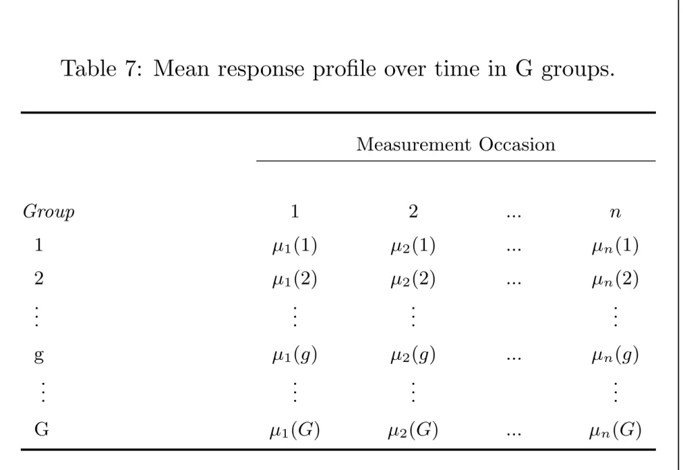
Hypotheses concerning response profiles

Given a sequence of n repeated measures on a number of distinct groups of individuals, three main questions:

1. Are the mean response profiles similar in the groups, in the sense that the mean response profiles are parallel? This is a question that concerns the group _× time

interaction effect; see Figure 7(a).

2. Assuming mean response profiles are parallel, are the means constant over time, in the sense that the mean response profiles are flat?

This is a question that concerns the time effect; see Figure 7(b).

3. Assuming that the population mean response profiles are parallel, are they also at the same level in the sense that the mean response profiles for the groups coincide?

This is a questions that concerns the group effect; see Figure 7(c).

1 2 3 4 Time Expected Response (a) Group 1 Group 2 1 2 3 4 Time Expected Response (b) Group 1 Group 2 1 2 3 4 Time Expected Response (c) Group 1 Group 2

Table 7: Mean response profile over time in G groups. Measurement Occasion Group 1 2 ... n 1 µ1(1) µ2(1) ... µn(1) 2 µ1(2) µ2(2) ... µn(2) .. . ... ... ... g µ1(g) µ2(g) ... µn(g) .. . ... ... ... G µ1(G) µ2(G) ... µn(G)

Consider two-group case: G = 2

Define ∆_j = µ_j(1) ₋ µ_j(2), j = 1, ..., n.

With G = 2, the first hypothesis in an analysis of response profiles can be expressed as:

No group _× time interaction effect:

H₀ : ∆₁ = ∆₂ = _{· · ·} = ∆_n, (n-1 degrees of freedom) With G _≥ 2, the test of the null hypothesis of no group _× time interaction effect has (G ₋ 1) _× (n ₋ 1) degrees of freedom.

Focus of analysis is on a global test of the null hypothesis that mean response profiles are parallel.

This question concerns the group _× time interaction effect. In testing this hypothesis, both group and time are regarded as categorical covariates (analogous to two-way ANOVA).

Analysis of response profiles can be specified as a regression model with “indicator variables” for group and time.

However, correlation and variability among repeated measures on the same individuals must be properly accounted for.

Dummy or Indicator Variable Coding:

Consider a factor with k levels:

Define X₁ = 1 if measurement or subject belongs to level 1, and 0 otherwise.

Define X₂ = 1 if measurement or subject belongs to level 2, and 0 otherwise.

Define X₃, ..., X_k similarly.

Note: In model with intercept term, we only require k ₋ 1 indicator variables. The choice of omitted indicator variable (e.g., X₁) determines what level of the factor is the

Level X₂ X₃ X₄ . . . X_k 1 0 0 0 . . . 0 2 1 0 0 . . . 0 3 0 1 0 . . . 0 4 0 0 1 . . . 0 .. . ... ... ... ... ... ... ... k 0 0 0 . . . 1

For example, this leads to a simple way of expressing the mean response in a regression model (with intercept β₁):

Y_ij = β₁ + β₂X_2ij + _{· · ·} + β_kX_kij + _ij

or (equivalently)

Note:

Mean response for level 1: µ₁ = β₁

Mean response for level 2: µ₂ = β₁ + β₂

.. .

Mean response for level k: µ_k = β₁ + β_k

Equivalently:

Level 2 versus Level 1 = β₂

Level 3 versus Level 1 = β₃

..

. ...

Choice of Reference Level

The usual choice of reference group:

(i) A natural baseline or comparison group, and/or

(ii) group with largest sample size

In longitudinal data setting, the “baseline” or first

In summary, analysis of response profiles can be specified as a regression model with “indicator variables” for group and

time.

The global test of the null hypothesis of parallel profiles

translates into a hypothesis concerning regression coefficients for the group _× time interaction being equal to zero.

Beyond testing the null hypothesis of parallel profiles, the estimated regression coefficients have meaningful

Treatment of Lead-Exposed Children Trial In the TLC Trial there are two groups (placebo and

succimer) and four measurement occasions (week 0, 1, 4, 6). Let X₁ = 1 for all children at all occasions.

Creating indicator variables for group and time: Group:

Let X₂ = 1 if child randomized to succimer, X₂ = 0 otherwise.

Time:

Let X₃ = 1 if measurement at week 1, X₃ = 0 otherwise Let X4 = 1 if measurement at week 4, X4 = 0 otherwise

Analysis of response profiles model can be expressed as:

Y = β1+β2X2+β3X3+β4X4+β5X5+β6X2∗X3+β7X2∗X4+β8X2∗X5+e

Test of group _× time interaction: H₀ : β₆ = β₇ = β₈ = 0.

The analysis must also account for the correlation among repeated measures on the same child.

The analysis of response profiles estimates separate variances for each occasion (4 variances) and six pairwise correlations.

Table 8: Estimated covariance matrix for the blood lead levels at baseline, week 1, week 4, and week 6 for the children from the TLC trial. Covariance Matrix 25.2 19.1 19.4 17.2 19.1 44.3 35.3 27.5 19.4 35.3 48.9 31.4 17.2 27.5 31.4 43.6

Note the discernible increase in the variability in blood lead levels from pre- to post-randomization.

This increase in variability from baseline is probably due to:

(1) given the treatment group assignment, there may be

natural heterogeneity in the individual response trajectories over time,

(2) the trial had an inclusion criterion that blood lead levels at baseline were in the range of 20-44 micrograms/dL.

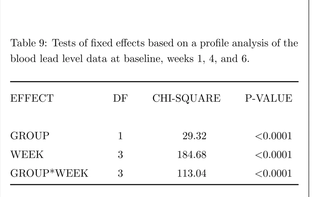
Table 9: Tests of fixed effects based on a profile analysis of the blood lead level data at baseline, weeks 1, 4, and 6.

EFFECT DF CHI-SQUARE P-VALUE

GROUP 1 29.32 <0.0001

WEEK 3 184.68 <0.0001

Test of the group _× time interaction is based on

(multivariate) Wald test (comparison of estimates to SEs).

In TLC trial, question of main interest concerns comparison of groups in terms of patterns of change from baseline.

This question translates into test of group _× time interaction. The test of the group _× time interaction yields a Wald

statistic of 113 with 3 degrees of freedom (p < 0.001).

Because this is a global test, it indicates that groups differ but does not tell us how they differ.

Recall, analysis of response profiles model can be expressed as:

Y = β1+β2X2+β3X3+β4X4+β5X5+β6X2∗X3+β7X2∗X4+β8X2∗X5+e

Test of group _× time interaction: H₀ : β₆ = β₇ = β₈ = 0.

The 3 single df contrasts for group _× time interaction have

direct interpretations in terms of group comparisons of changes from baseline.

They indicate that children treated with succimer have greater decrease in mean blood lead levels from baseline at all occasions when compared to children treated with placebo (see Table 10).

Table 10: Estimated regression coefficients and standard errors based on a profile analysis of the blood lead level data.

PARAMETER GROUP WEEK ESTIMATE SE Z

INTERCEPT 26.27 0.71 36.99 GROUP A 0.27 1.00 0.27 WEEK 1 -1.61 0.79 -2.03 WEEK 4 -2.21 0.84 -2.63 WEEK 6 -3.03 0.83 -3.65 GROUP*WEEK A 1 -11.43 1.12 -16.20 GROUP*WEEK A 4 -9.08 1.19 -7.64 GROUP*WEEK A 6 -3.84 1.17 -3.27

Strengths and Weaknesses of Analysis of Response Profiles

Strengths:

Allows arbitrary patterns in the mean response over time and arbitrary patterns in the covariance.

Analysis has a certain robustness since potential risks of bias due to misspecification of models for mean and covariance are minimal.

Drawbacks:

Requirement that the longitudinal design be balanced. Analysis cannot incorporate mistimed measurements.

Analysis ignores the time-ordering (time trends) of the repeated measures in a longitudinal study – “occasion” is regarded as a qualitative factor.

Produces omnibus tests of effects that may have low power to detect group differences in specific trends in the mean

response over time (e.g., linear trends in the mean response).

The number of estimated parameters, G _× n mean

parameters and n(n₂+1) covariance parameters, grows rapidly with the number of measurement occasions.

Further Reading:

Fitzmaurice GM, Laird NM and Ware JH. (2004) Applied Longitudinal Analysis. Wiley.

– Chapter 3 (Sections 3.1, 3.2, 3.4, 3.5) – Chapter 4 (Sections 4.1, 4.2, 4.4, 4.5) – Chapter 5 (Sections 5.1-5.4, 5.8, 5.9)

APPLIED LONGITUDINAL ANALYSIS

MODELLING THE MEAN:

PARAMETRIC CURVES

Fitting parametric or semi-parametric curves to longitudinal data can be justified on substantive and statistical grounds.

Substantively, in many studies true underlying mean response process changes over time in a relatively smooth,

monotonically increasing/decreasing pattern.

Fitting parsimonious models for mean response results in statistical tests of covariate effects (e.g., treatment _× time interactions) with greater power than in profile analysis.

Polynomial Trends in Time

Describe the patterns of change in the mean response over time in terms of simple polynomial trends.

The means are modelled as an explicit function of time.

This approach can handle highly unbalanced designs in a relatively seamless way.

For example, mistimed measurements are easily incorporated in the model for the mean response.

Linear Trends over Time

Simplest possible curve for describing changes in the mean response over time is a straight line.

Slope has direct interpretation in terms of a constant change in mean response for a single unit change in time.

Consider two-group study comparing treatment and control, where changes in mean response are approximately linear:

E (Y_ij) = β₁ + β₂Time_ij + β₃Group_i + β₄Time_{ij ×} Group_i,

where Group_i = 1 if ith individual assigned to treatment, and Group_i = 0 otherwise; and Time_ij denotes measurement time for the jth measurement on ith individual.

Model for the mean for subjects in control group:

E (Y_ij) = β₁ + β₂Time_ij,

while for subjects in treatment group,

E (Y_ij) = (β₁ + β₃) + (β₂ + β₄) Time_ij.

Thus, each group’s mean response is assumed to change linearly over time (see Figure 8).

0 1 2 3 4 5

Time

Expected Response

Group 1

Group 2

Figure 8: Graphical representation of model with linear trends for two groups.

Quadratic Trends over Time

When changes in the mean response over time are not linear, higher-order polynomial trends can be considered.

For example, if the means are monotonically increasing or decreasing over the course of the study, but in a curvilinear way, a model with quadratic trends can be considered.

In a quadratic trend model the rate of change in the mean response is not constant but depends on time.

Consider two-group study example:

E (Y_ij) = β₁ + β₂Time_ij + β₃Time2_ij + β₄Group_i

+ β₅Time_{ij ×} Group_i + β₆Time2_{ij ×} Group_i.

Model for subjects in control group:

E (Yij) = β1 + β2Timeij + β3Time2_ij;

while model for subjects in treatment group:

0 1 2 3 4 5

Time

Expected Response

Group 1

Group 2

Figure 9: Graphical representation of model with quadratic trends for two groups.

Note: mean response changes at different rate, depending upon Time_ij.

Rate of change in control group is β₂ + 2β₃Time_ij

(derivation of this instantaneous rate of change requires familiarity with calculus).

Thus, early in the study when Time_ij = 1, rate of change is

β₂ + 2β₃; while later in the study, say Time_ij = 4, rate of change is β₂ + 8β₃.

Regression coefficients, (β₂ + β₅) and (β₃ + β₆), have similar interpretations for treatment group.

“Centering”

To avoid problems of collinearity it is advisable to “center” Timej on its mean value prior to the analysis.

Replace Time_j by its deviation from the mean of (Time₁,Time₂,...,Time_n).

Note: centering of Time_ij at individual-specific values (e.g., the mean of the ni measurement times for ith individual)

should be avoided, as the interpretation of the intercept becomes meaningless.

Linear Splines

If simplest possible curve is a straight line, then one way to extend the curve is to have sequence of joined line segments that produces a piecewise linear pattern.

Linear spline models provide flexible way to accommodate many non-linear trends that cannot be approximated by simple polynomials in time.

Basic idea: Divide time axis into series of segments and

consider piecewise-linear trends, having different slopes but joined at fixed times.

Locations where lines are tied together are known as “knots”. Resulting piecewise-linear curve is called a spline.

0 1 2 3 4 5

Time

Expected Response

Group 1

Group 2

Figure 10: Graphical representation of model with linear splines for two groups, with common knot.

The simplest possible spline model has only one knot.

For two-group example, linear spline model with knot at t∗:

E (Y_ij) = β₁ + β₂Time_ij + β₃(Time_{ij −} t∗)₊ + β₄Group_i

+ β₅Time_{ij ×} Group_i + β₆(Time_{ij −} t∗)_{+ ×} Group_i,

where (x)+ is defined as a function that equals x when x is

positive and is equal to zero otherwise.

Thus, (Time_{ij −} t∗)₊ is equal to (Time_{ij −} t∗) when Time_ij > t∗

and is equal to zero when Time_{ij ≤} t∗.

Model for subjects in control group:

E (Y_ij) = β₁ + β₂Time_ij + β₃(Time_{ij −} t∗)₊.

When expressed in terms of mean response prior/after t∗:

E (Y_ij) = β₁ + β₂Time_ij, Time_{ij ≤} t∗;

E (Y_ij) = (β_{1 −} β₃t∗) + (β₂ + β₃)Time_ij, Time_ij > t∗.

Model for subjects in treatment group:

E (Yij) = (β1 + β4) + (β2 + β5)Time_ij + (β3 + β6)(Time_ij − t∗)+.

When expressed in terms of mean response prior/after t∗:

E (Y_ij) = (β₁ + β₄) + (β₂ + β₅)Time_ij, Time_{ij ≤} t∗;

E (Y_ij) = [(β₁ + β₄) ₋ (β₃ + β₆)t∗)]

Case Study 1: Vlagtwedde-Vlaardingen Study Epidemiologic study on risk factors for chronic obstructive lung disease.

Sample participated in follow-up surveys approximately every 3 years for up to 19 years.

Pulmonary function was determined by spirometry: FEV₁.

We focus on subset of 133 residents aged 36 or older at entry into study and whose smoking status did not change during follow-up.

0 5 10 15 20 2.4 2.6 2.8 3 3.2 3.4 3.6 Time (years)

Mean FEV1 (liters)

Former Smokers Current Smokers

Figure 11: Mean FEV₁ at baseline (year 0), year 3, year 6, year 9, year 12, year 15, and year 19 in the current and former smoking exposure groups.

First we consider a linear trend in the mean response over time, with intercepts and slopes that differ for the two smoking exposure groups.

We assume an unstructured covariance matrix. Based on the REML estimates of the regression

coefficients in Table 11, the mean response for former smokers is

E(Yij) = 3.507 ₋ 0.033 Time_ij,

while for current smokers,

E(Yij) = (3.507 − 0.262) − (0.033 + 0.005) Timeij

Table 11: Estimated regression coefficients for linear trend model for FEV₁ data from the Vlagtwedde-Vlaardingen study.

Variable Smoking Group Estimate SE Z

Intercept 3.5073 0.1004 34.94

Smokei Current −0.2617 0.1151 −2.27

Timeij −0.0332 0.0031 −10.84

Thus, both groups have a significant decline in mean FEV₁ over time.

But there is no discernible difference between the two smoking exposure groups in the constant rate of change.

That is, the Smoke_i × Time_ij interaction (i.e., the comparison

of the two slopes) is not significant, with

Z = ₋1.42, p > 0.15.

But is the rate of change constant over time?

Adequacy of linear trend model can be assessed by including higher-order polynomial trends.

For example, we can consider a model that allows quadratic trends for changes in FEV₁ over time.

Recall that linear trend model is nested within quadratic trend model.

The maximized log-likelihoods for models with linear and quadratic trends are presented in Table 12.

LRT test statistic, based on ML not REML, can be

compared to a chi-squared distribution with 2 degrees of freedom (or 6, the number of parameters in the

quadratic trend model, minus 4, the number of parameters in the linear trend model).

Table 12: Maximized (ML) log-likelihoods for models with linear and quadratic trends for FEV₁ data from the Vlagtwedde-Vlaardingen study.

Model ₋2 (ML) Log-Likelihood

Quadratic Trend Model 237.2

Linear Trend Model 238.5

LRT comparing quadratic and linear trend models, produces

G2 = 1.3, with 2 degrees of freedom (p > 0.50).

Thus, when compared to quadratic trend model, linear trend model appears to be adequate.

Finally, for illustrative purposes, we can make a comparison with a cubic trend model.

This produces LRT statistic, G2 = 4.4, with 4 degrees of freedom (p > 0.35), indicating again that the linear trend model is adequate.

Case Study 2: Treatment of Lead-Exposed Children Trial

Recall data from TLC trial:

Children randomized to placebo or Succimer.

Measures of blood lead level at baseline, 1, 4 and 6 weeks.

The sequence of means over time in each group is displayed in Figure 12.

0 2 4 6 10 15 20 25 30 Time (weeks)

Mean blood lead level (mcg/dL)

Placebo Succimer

Figure 12: Mean blood lead levels at baseline, week 1, week 4, and week 6 in the succimer and placebo groups.

Given that there are non-linearities in the trends over time,

higher-order polynomial models (e.g., a quadratic trend model) could be fit to the data.

Alternatively, we can accommodate the non-linearity with a piecewise linear model with common knot at week 1,

E (Yij) = β1 + β2 Weekij + β3 (Weekij − 1)+ + β4 Groupi × Weekij

+ β5 Groupi × (Weekij − 1)+,

where Group_i = 1 if assigned to succimer, and Group_i = 0

In this piecewise linear model, means for subjects in placebo group are

E (Yij) = β1 + β2 Weekij + β3 (Weekij − 1)+,

while in the succimer group

E(Yij) = β1 + (β2 + β4) Weekij + (β3 + β5) (Weekij − 1)+.

Because of randomization, assume a common mean at baseline (no Group main effect).

Table 13: Estimated regression coefficients and standard errors based on a piecewise linear model, with knot at week 1.

Variable Group Estimate SE Z

Intercept 26.3422 0.4991 52.78

Weekij −1.6296 0.7818 −2.08

(Weekij − 1)+ 1.4305 0.8777 1.63

Group _× Weekij A −11.2500 1.0924 −10.30

When expressed in terms of mean response prior to/after week 1, estimated means in the placebo group are

b

µ_ij = βb₁ + βb₂ Week_ij, Week_ij ≤ 1;

b

µ_ij = (βb_{1 −} βb₃) + (βb₂ + βb₃) Week_ij, Week_ij > 1.

Thus, in the placebo group, slope prior to week 1 is

b

β₂ = ₋1.63 and following week 1 is (βb₂ + βb₃) = ₋1.63 + 1.43 = ₋0.20.

Similarly, when expressed in terms of the mean response prior to and after week 1, the estimated means for subjects in the succimer group are given by

b

µ_ij = βb₁ + (βb₂ + βb₄) Week_ij, Week_ij ≤ 1;

b

µ_ij = βb_{1 −} (βb₃ + βb₅)

Estimates of mean blood lead levels for placebo and succimer groups are presented in Table 14.

The estimated means appear to adequately fit observed mean response profiles for two treatment groups.

Note piecewise linear and quadratic trend models (with common intercept for two groups) are not nested.

Because they have same number of parameters, their

log-likelihoods (LL) can be directly compared: piecewise linear model fits better than quadratic trend model (₋2 ML LL =

2436.2 for piecewise linear model versus ₋2 ML LL = 2551.7 for quadratic trend model).

Table 14: Estimated mean blood lead levels for placebo and succimer groups from linear spline model (knot at week 1). Observed means in parentheses.

Group Week 0 Week 1 Week 4 Week 6

Succimer 26.3 13.5 16.7 19.1

(26.5) (13.5) (15.5) (20.8)

Placebo 26.3 24.7 24.1 23.7

Further Reading:

Fitzmaurice GM, Laird NM and Ware JH. (2004) Applied Longitudinal Analysis. Wiley.

APPLIED LONGITUDINAL ANALYSIS

MODELLING THE COVARIANCE

require modelling: mean response over time and covariance. Although these two aspects of the data can be modelled

separately, they are interrelated.

Choice of models for mean response and covariance are interdependent.

A model for the covariance must be chosen on the basis of some assumed model for the mean response.

Covariance between any pair of residuals, say [Y_{ij −} µ_ij(β)] and [Y_{ik −} µ_ik(β)], depends on the model for the mean, i.e., depends on β.

Modelling the Covariance

Three broad approaches can be distinguished:

(1) “unstructured” or arbitrary pattern of covariance

(2) covariance pattern models

Unstructured Covariance

Appropriate when design is “balanced” and number of measurement occasions is relatively small.

No explicit structure is assumed other than homogeneity of covariance across different individuals, Cov(Y_i) = Σ_i = Σ.

Chief advantage: no assumptions made about the patterns of variances and covariances.

With n measurement occasions, “unstructured” covariance matrix has n×(n₂+1) parameters:

the n variances and n _× (n ₋ 1)/2 pairwise covariances (or correlations), Cov(Y_i) =         σ₁2 σ₁₂ . . . σ_1n σ₂₁ σ₂2 . . . σ_2n .. . ... . .. ... σ_n1 σ_n2 . . . σ_n2         .

Potential drawbacks:

Number of covariance parameters grows rapidly with the number of measurement occasions:

For n = 3 number of covariance parameters is 6 For n = 5 number of covariance parameters is 15 For n = 10 number of covariance parameters is 55

When number of covariance parameters is large, relative to sample size, estimation is likely to be very unstable.

Use of an unstructured covariance is appealing only when N

is large relative to n×(n₂+1).

Unstructured covariance is problematic when there are mistimed measurements.

Covariance Pattern Models

When attempting to impose some structure on the covariance, a subtle balance needs to be struck.

With too little structure there may be too many parameters to be estimated with limited amount of data.

With too much structure, potential risk of model

misspecification and misleading inferences concerning β. Classic tradeoff between bias and variance.

Covariance pattern models have their basis in models for serial correlation originally developed for time series data.

Compound Symmetry

Assumes variance is constant across occasions, say σ2, and Corr(Y_ij, Y_i,k) = ρ for all j and k.

Cov(Y_i) = σ2            1 ρ ρ . . . ρ ρ 1 ρ . . . ρ ρ ρ 1 . . . ρ .. . ... ... . .. ... ρ ρ ρ . . . 1            .

Parsimonious: two parameters regardless of number of measurement occasions.

Strong assumptions about variance and correlation are usually not valid with longitudinal data.

Toeplitz

Assumes variance is constant across occasions, say σ2, and Corr(Y_ij, Y_i,j+k) = ρ_k for all j and k.

Cov(Y_i) = σ2            1 ρ₁ ρ₂ . . . ρ_n−1 ρ₁ 1 ρ₁ . . . ρ_n−2 ρ₂ ρ₁ 1 . . . ρ_n−3 .. . ... ... . .. ... ρ_n−1 ρ_n−2 ρ_n−3 . . . 1            .

Assumes correlation among responses at adjacent measurement occasions is constant, ρ₁.

Toeplitz only appropriate when measurements are made at equal (or approximately equal) intervals of time.

Toeplitz covariance has n parameters (1 variance parameter, and n ₋ 1 correlation parameters).

A special case of the Toeplitz covariance is the (first-order) autoregressive covariance.

Autoregressive

Assumes variance is constant across occasions, say σ2, and Corr(Y_ij, Y_i,j+k) = ρk for all j and k, and ρ _≥ 0.

Cov(Y_i) = σ2            1 ρ ρ2 . . . ρn−1 ρ 1 ρ . . . ρn−2 ρ2 ρ 1 . . . ρn−3 .. . ... ... . .. ... ρn−1 ρn−2 ρn−3 . . . 1            .

Parsimonious: only 2 parameters, regardless of number of measurement occasions.

Only appropriate when the measurements are made at equal (or approximately equal) intervals of time.

Compound symmetry, Toeplitz and autoregressive

covariances assume variances are constant across time.

This assumption can be relaxed by considering versions of these models with heterogeneous variances, Var(Y_ij) = σ_j2. A heterogeneous autoregressive covariance pattern:

Cov(Y_i) =          σ2 1 ρσ1σ2 ρ 2_σ 1σ3 . . . ρn−1σ1σn ρσ1σ2 σ₂2 ρσ2σ3 . . . ρn−2σ2σ_n ρ2σ1σ3 ρσ2σ3 σ₃2 . . . ρn−3σ3σn .. . ... ... . .. ... ρn₋1 σ1σn ρn−2σ2σn ρn−3σ3σn . . . σ_n2          ,

and has n + 1 parameters (n variance parameters and 1 correlation parameter).

Banded

Assumes correlation is zero beyond some specified interval.

For example, a banded covariance pattern with a band size of 3 assumes that Corr(Y_ij, Y_i,j+k) = 0 for k _≥ 3.

It is possible to apply a banded pattern to any of the covariance pattern models considered so far.

A banded Toeplitz covariance pattern with a band size of 2 is given by, Cov(Yi) = σ2            1 ρ₁ 0 . . . 0 ρ₁ 1 ρ₁ . . . 0 0 ρ₁ 1 . . . 0 .. . ... ... . .. ... 0 0 0 . . . 1            , where ρ₂ = ρ₃ = _{· · ·} = ρ_n−1 = 0.

Banding makes very strong assumption about how quickly the correlation decays to zero with increasing time separation.

Exponential

When measurement occasions are not equally-spaced over time, autoregressive model can be generalized as follows. Let _{t_i1, ..., t_in} denote the observation times for the ith

individual and assume that the variance is constant across all measurement occasions, say σ2, and

Corr(Y_ij, Y_ik) = ρ|tij−tik|,

for ρ _≥ 0.

Correlation between any pair of repeated measures decreases exponentially with the time separations between them.

Referred to as “exponential” covariance because it can be re-expressed as

Cov(Yij, Yik) = σ2ρ|tij−tik|

= σ2 exp (₋θ _|t_{ij −} t_ik|) ,

where θ = ₋ log(ρ) or ρ = exp (₋θ) for θ _≥ 0.

Exponential covariance model is invariant under linear transformation of the time scale.

If we replace t_ij by (a + bt_ij) (e.g., if we replace time

measured in “weeks” by time measured in “days”), the same form for the covariance matrix holds.

Choice among Covariance Pattern Models

Choice of models for covariance and mean are interdependent.

Choice of model for covariance should be based on a

“maximal” model for the mean that minimizes any potential misspecification.

With balanced designs and a very small number of discrete covariates, choose “saturated model” for the mean response.

Saturated model: includes main effects of time (regarded as a within-subject factor) and all other main effects, in addition to their two- and higher-way interactions.

Maximal model should be in a certain sense the most elaborate model for the mean response that we would consider from a subject-matter point of view.

Once maximal model has been chosen, residual variation and covariation can be used to select appropriate model for

covariance.

For nested covariance pattern models, a likelihood ratio test statistic can be constructed that compares “full” and

Recall: two models are said to be nested when the “reduced” model is a special case of the “full” model.

For example, compound symmetry model is nested within the Toeplitz model, since if the former holds the latter must

necessarily hold, with ρ₁ = ρ₂ = _{· · ·} = ρ_n−1.

Likelihood ratio test is obtained by taking twice the

difference in the respective maximized REML log-likelihoods,

G2 = 2(bl_{full −} bl_red),

and comparing statistic to a chi-squared distribution with df equal to difference between the number of covariance

To compare non-nested model, an alternative approach is the Akaike Information Criterion (AIC).

According to the AIC, given a set of competing models for the covariance, one should select the model that minimizes

AIC = ₋2(maximized log-likelihood) + 2(number of parameters)

= ₋2(bl ₋ c),

where bl is the maximized REML log-likelihood and c is the number of covariance parameters.

Exercise Therapy Trial

• subjects were assigned to one of two weightlifting programs to increase muscle strength.

• treatment 1: number of repetitions of the exercises was increased as subjects became stronger.

• treatment 2, number of repetitions was held constant but amount of weight was increased as subjects became

stronger.

• Measurements of body strength were taken at baseline and on days 2, 4, 6, 8, 10, and 12.

• We focus only on measures of strength obtained at baseline (or day 0) and on days 4, 6, 8, and 12.

Before considering models for the covariance, it is necessary to choose a maximal model for the mean response.

We chose maximal model to be the saturated model for the mean.

First, we consider an unstructured covariance matrix.

Note that the variance is larger by the end of the study when compared to the variance at baseline.

Correlations decrease as the time separation between the repeated measures increases.

Table 15: Estimated unstructured covariance matrix for the strength data at baseline, day 4, day 6, day 8, and day 12.

Day 0 4 6 8 12 0 9.668 10.175 8.974 9.812 9.407 4 10.175 12.550 11.091 12.580 11.928 6 8.974 11.091 10.642 11.686 11.101 8 9.812 12.580 11.686 13.990 13.121 12 9.407 11.928 11.101 13.121 13.944

Table 16: Estimated unstructured correlation matrix for the strength data at baseline, day 4, day 6, day 8, and day 12.

Day 0 4 6 8 12 0 1.0000 0.9237 0.8847 0.8437 0.8102 4 0.9237 1.0000 0.9597 0.9494 0.9017 6 0.8847 0.9597 1.0000 0.9577 0.9113 8 0.8437 0.9494 0.9577 1.0000 0.9394 12 0.8102 0.9017 0.9113 0.9394 1.0000

Despite apparent increase in variance over time, we consider an autoregressive model for the correlation.

It results in the following estimates of the variance and correlation parameters, _bσ2 = 11.87 and ρ_b = 0.94.

This model is not very appropriate as data are unequally spaced over time.

Consider exponential model for the covariance, where

Corr(Y_ij, Y_ik) = ρ|tij−tik|,

for ti = (0, 4, 6,8, 12) for all subjects.

Table 17: Estimated autoregressive correlation matrix for the strength data at baseline, day 4, day 6, day 8, and day 12.

Day 0 4 6 8 12 0 1.0000 0.9402 0.8839 0.8311 0.7813 4 0.9402 1.0000 0.9402 0.8839 0.8311 6 0.8839 0.9402 1.0000 0.9402 0.8839 8 0.8311 0.8839 0.9402 1.0000 0.9402 12 0.7813 0.8311 0.8839 0.9402 1.0000

Table 18: Estimated exponential correlation matrix for the strength data at baseline, day 4, day 6, day 8, and day 12.

Day 0 4 6 8 12 0 1.0000 0.9169 0.8780 0.8408 0.7709 4 0.9169 1.0000 0.9576 0.9169 0.8408 6 0.8780 0.9576 1.0000 0.9576 0.8780 8 0.8408 0.9169 0.9576 1.0000 0.9169 12 0.7709 0.8408 0.8780 0.9169 1.0000

There is a hierarchy among the models: autoregressive and exponential are both nested within unstructured.

The autoregressive and exponential models are not nested but have the same number of parameters.

Any comparison between these two models can be made directly in terms of their maximized log-likelihoods.

LRT comparing autoregressive and unstructured covariance,

G2 = 621.1 ₋ 597.3 = 23.8,

with 13 (or 15 - 2) degrees of freedom (p < 0.05).

There is evidence that the autoregressive model does not provide an adequate fit to the covariance.

LRT comparing exponential and unstructured covariance, yields

G2 = 618.5 ₋ 597.3 = 21.2,

and when compared to a chi-squared distribution with 13 degrees of freedom, p > 0.05.

Exponential covariance provides an adequate fit to the data.

Also, in terms of AIC, the exponential model minimizes this criterion.

Table 19: Comparison of the maximized (REML) log-likelihoods and AIC for the covariance pattern models for the strength data from the exercise therapy trial.

Covariance Pattern Model -2 (REML) Log-Likelihood AIC

Unstructured 597.3 627.3

Autoregressive 621.1 625.1

Strengths/Weaknesses of Covariance Pattern Models Covariance pattern models attempt to characterize the

covariance with a relatively small number of parameters. However, many models (e.g., autoregressive, Toeplitz, and banded) appropriate only when repeated measurements are obtained at equal intervals and cannot handle irregularly timed measurements.

While there is a large selection of models for correlations, choice of models for variances is limited.

They are not well-suited for modelling data from inherently unbalanced longitudinal designs.

Further Reading:

Fitzmaurice GM, Laird NM and Ware JH. (2004) Applied Longitudinal Analysis. Wiley.

APPLIED LONGITUDINAL ANALYSIS