Contents lists available atScienceDirect
Pattern Recognition
journal homepage:www.elsevier.com/locate/pr
Explaining nonlinear classi
fi
cation decisions with deep Taylor
decomposition
Grégoire Montavon
a,⁎, Sebastian Lapuschkin
b, Alexander Binder
c, Wojciech Samek
b,⁎,
Klaus-Robert Müller
a,d,⁎⁎aDepartment of Electrical Engineering & Computer Science, Technische Universität Berlin, Marchstr. 23, Berlin 10587, Germany bDepartment of Video Coding & Analytics, Fraunhofer Heinrich Hertz Institute, Einsteinufer 37, Berlin 10587, Germany
cInformation Systems Technology & Design, Singapore University of Technology and Design, 8 Somapah Road, Building 1, Level 5, 487372, Singapore dDepartment of Brain & Cognitive Engineering, Korea University, Anam-dong 5ga, Seongbuk-gu, Seoul 136-713, South Korea
A R T I C L E I N F O
Keywords:Deep neural networks Heatmapping Taylor decomposition Relevance propagation Image recognition
A B S T R A C T
Nonlinear methods such as Deep Neural Networks (DNNs) are the gold standard for various challenging machine learning problems such as image recognition. Although these methods perform impressively well, they
have a significant disadvantage, the lack of transparency, limiting the interpretability of the solution and thus
the scope of application in practice. Especially DNNs act as black boxes due to their multilayer nonlinear structure. In this paper we introduce a novel methodology for interpreting generic multilayer neural networks
by decomposing the network classification decision into contributions of its input elements. Although our focus
is on image classification, the method is applicable to a broad set of input data, learning tasks and network
architectures. Our method called deep Taylor decomposition efficiently utilizes the structure of the network by backpropagating the explanations from the output to the input layer. We evaluate the proposed method empirically on the MNIST and ILSVRC data sets.
1. Introduction
Nonlinear models have been used since the advent of machine learning (ML) methods and are integral part of many popular algorithms. They include, for example, graphical models [1], kernels [2,3], Gaussian processes[4], neural networks[5–7], boosting[8], or random forests[9]. Recently, a particular class of nonlinear methods, Deep Neural Networks (DNNs), revolutionized thefield of automated image classification by demonstrating impressive performance on large benchmark data sets[10–12]. Deep networks have also been applied successfully to other researchfields such as natural language proces-sing[13,14], human action recognition[15–17], or physics[18,19].
Although these models are highly successful in terms of perfor-mance, they have a drawback of acting like ablack boxin the sense that it is not clearhowandwhythey arrive at a particular classification decision. This lack of transparency is a serious disadvantage as it prevents a human expert from being able to verify, interpret, and understand the reasoning of the system. In this paper, we consider the
problem of explaining classification decisions of a machine learning model in terms of input variables. For instance, for image classification problems, the classifier should not only indicate whether an image of interest belongs to a certain category or not, but also explain what structures (e.g. pixels in the image) were the basis for its decision.
Linear models readily provide explanations in terms of input variables [20–22], however, due to their limited expressive power, they cannot be applied to complex tasks such as explaining image classifications. Explanation methods for complex nonlinear models such as convolutional neural networks can be categorized as follows: (1)functional approaches
[23]where the explanation results from the local analysis of the prediction function, for example, sensitivity analysis or Taylor series expansion, and (2)message passing approaches[24,25]that view the prediction as the output of a computational graph, and where the explanation is obtained by running a backward pass in that graph.
A main goal of this paper is to reconcile in the context of deep neural networks the functional and message passing approaches for producing these explanations.1Specifically, we view each neuron of a
http://dx.doi.org/10.1016/j.patcog.2016.11.008
Received 11 May 2016; Received in revised form 8 August 2016; Accepted 12 November 2016 ⁎Corresponding authors.
⁎⁎Corresponding author at: Department of Electrical Engineering & Computer Science, Technische Universität Berlin, Marchstr. 23, Berlin 10587, Germany
E-mail addresses:[email protected](G. Montavon),[email protected](S. Lapuschkin),[email protected](A. Binder), [email protected](W. Samek),[email protected](K.-R. Müller).
1Similarly, error backpropagation[26]used for training neural networks also offers both a function-based interpretation (gradient evaluation) and a message passing interpretation (chain-rule for derivatives).
Available online 30 November 2016
0031-3203/ © 2017 The Authors. Published by Elsevier Ltd.
This is an open access article under the CC BY license (http://creativecommons.org/licenses/BY/4.0/).
deep network as a function that can be expanded and decomposed on its input variables. The decompositions of multiple neurons are then aggregated or propagated backwards, resulting in a “deep Taylor decomposition”. Furthermore, we will show how the propagation rules derived from deep Taylor decomposition relate to those heuristically defined by[25].
Because of the theoretical focus of this paper, we do not perform a broader empirical comparison with other recently proposed methods for explanation, however, we refer to[27]for that matter.
1.1. Related work
There has been a significant body of work focusing on the analysis and understanding of nonlinear classifiers. Some methods seek to provide a globalunderstanding of the trained model, by measuring important characteristics of it, such as the noise and relevant dimen-sionality of its feature space(s) [28–30], its invariance to certain transformations of the data[31], the role of particular neurons[32], or its global decision structure[33,34]. Other methods focus instead on the interpretation ofindividualpredictions. The method proposed in [35] explains predictions in terms of input variables by locally evaluating the gradient of the decision function. Simonyan et al.[23] incorporate saliency information into the explanation by multiplying the gradient by the actual data point. To determine the importance of input variables for a particular prediction, Landecker et al. [36] proposed a contribution propagation approach for hierarchical net-works, applying at each unit of the network a propagation rule that obeys a conservation property.
Recent work has focused on the problem of understanding of state-of-the-art GPU-trained convolutional neural networks for image clas-sification[23–25,37], offering new insights into these highly complex models. The deconvolution method proposed by Zeiler and Fergus[24] was designed to visualize and understand the features of state-of-the-art convolutional neural networks with max-pooling and rectified linear units. The method performs a backpropagation pass on the network, where a set of rules is applied uniformly to all layers of the network, resulting in an assignment of values onto pixels. The method however does not aim to attribute a defined meaning to the assigned pixel values, except for the fact that they should form a visually interpretable pattern. For the same convolutional neural network models, the layer-wise relevance propagation method of Bach et al.[25]applies at each neuron of the network a propagation rule with a conservative property, resulting in an assignment of values onto pixels which is directly interpretable as their importance for the classification decision. While scoring high quantitatively[27], the choice of propagation rules was mainly heuristic and lacked a strong theoretical justification.
A theoretical foundation to the problem of measuring the impor-tance of input variables for a prediction, can be found in the Taylor decomposition of a nonlinear function. The approach was described by Bazen and Joutard[38] as a nonlinear generalization of the Oaxaca method in econometrics[21]. The idea was subsequently introduced in the context of image analysis [23,25] for the purpose of explaining machine learning classifiers.
As an alternative to propagation methods, spatial response maps [39] build heatmaps by looking at the neural network output while sliding the neural network in the pixel space. Attention models based on neural networks, trained to classify an image from only a few glimpses of it [40], readily provide a spatial interpretation for the classification decision. Similar models can also visualize what part of an image is relevant at a given time in some temporal context [41]. However, these dynamical models can be significantly more complex to design and train.
2. Pixel-wise decomposition of a function
In this section, we describe the general concept of explaining a
neural network decision by decomposing the function value (i.e. neural network output) onto the input variables in an amount that matches the respective relevance of these input variables to the function value. After enumerating a certain number of desirable properties of a decomposition, we will present in Sections 2.1 and 2.2 two simple solutions to this problem. Because all subsequent empirical evaluations focus on the problem of image recognition, we call the input variables “pixels”, and use the letterpfor indexing them. Also, we employ the term“heatmap”to designate the set relevance scores assigned to pixels of an image. Despite the image-related terminology, the concept is applicable to other input domains such as vector spaces, time series, or more generally any type of input domain whose elements can be processed by a neural network2.
Let us consider a positive-valued function f:d→+. In the
context of image classification, the inputx∈d of this function is an
image. The image can be viewed as a set of pixel valuesx= { }xp where
pdenotes a particular pixel. The functionf( )x quantifies the presence of a certain type of object(s) in the image. A function value f( ) = 0x indicates an absence of it. On the other hand, a function valuef( ) > 0x expresses its presence with a certain degree of certainty, or in a certain amount.
We would like to associate to each pixelpin the image arelevance scoreRp( )x, that indicates for an imagex to what extent the pixelp contributes to explaining the classification decisionf( ). The relevancex of each pixel can be stored in a heatmap denoted byR x( ) = {Rp( )}x of same dimensions asxand can be visualized as an image. A heatmap-ping should satisfy properties that we define below:
Definition 1. A heatmapping R x( ) is conservative if the sum of assigned relevances in the pixel space corresponds to the total relevance detected by the model:
∑
x f x R x ∀ : ( ) = ( ).p p
Definition 2.A heatmappingR x( )ispositiveif all values forming the heatmap are greater or equal to zero, that is:
x p R x ∀ , : p( ) ≥ 0
The first property ensures that the total redistributed relevance corresponds to the extent to which the object in the input image is detected by the functionf( ). The second property forces the heatmap-x ping to assume that the model is devoid of contradictory evidence (i.e. no pixels can be in contradiction with the presence or absence of the detected object in the image). These two properties can be combined into the notion ofconsistency:
Definition 3.A heatmappingR x( )isconsistentif it is conservative
andpositive. That is, it is consistent if it complies withDefinitions 1 and 2.
In particular, a consistent heatmap is forced to satisfy
x R x
f 0
( ( ) = 0) ⇒ ( ( ) = ). That is, in absence of an object to detect, the relevance is forced to be zero everywhere in the image (i.e. empty heatmap), and not simply to have negative and positive relevance in same amount. We will useDefinition 3as a formal tool for assessing the correctness of the heatmapping techniques proposed in this paper. It was noted by [25] that there may be multiple heatmapping techniques that satisfy a particular definition. For example, we can consider a heatmapping that assigns for all images the relevance uniformly onto the pixel grid:
x x
p R
d f ∀ : p( ) = 1· ( ),
(1)
where d is the number of input dimensions. Alternately, we can consider a heatmapping where all relevance is assigned to the first pixel: ⎧ ⎨ ⎩ x x R ( ) = f( ) ifp= 1st pixel 0 else. p (2) Both(1) and (2)are consistent in the sense ofDefinition 3, however they lead to different relevance assignments. In practice, it is not possible to specify explicitly all properties that a heatmapping techni-que should satisfy. In the following, we give two meaningful examples of decompositions that comply with the definitions above.
2.1. Natural decomposition
A natural decomposition can be defined as a decomposition that is obtained directly from the structure of the prediction. Consider, for example, the prediction function
∑
x f( ) = σ x( ), p p p (3) where{ }σp is a set of positive nonlinear functions applying to eachpixel. The relevance of each input variable can be identified as elements of the sum[22]:
x
Rp( ) =σ xp( ).p
If there exists for each pixel a deactivated statex∼psuch thatσ xp( ) = 0∼p ,
then, the relevance scoreRp( )x can be interpreted as the effect on the prediction of deactivating pixelp. A pixel whose deactivation would cause a large drop in function value is therefore modeled as relevant.
Fig. 1illustrates on a simple two-dimensional function the diff er-ence between this decomposition technique and another frequently used explanation technique called sensitivity analysis [44], which explains the prediction as locally evaluated squared partial derivatives. We can observe that sensitivity analysis is not related to the function value and is discontinuous in some regions of the input space. The natural decomposition, on the other hand, is continuous and also incorporates the function value, as evidenced by the continuously varying size and direction of the arrows.
While this example motivates the importance of distinguishing between decomposition and sensitivity, functions like the one of Eq.(3) are typically not expressive enough to model the high complexity of input-output relations observed in real data.
2.2. Taylor decomposition
Moving to the general case of arbitrary differentiable functions x
f( ), we introduce a decomposition method based on the Taylor expansion of the function at some well-chosen root point x∼. A root point is a point where f( ) = 0x∼ . The first-order Taylor expansion of
x f( )is given by ⎛ ⎝ ⎜ ⎞⎠⎟
∑
x x x x x f f f ε f x x x ε ( ) = ( ) + ∂ ∂ ·( − ) + = 0 + ∂ ∂ ·( − ) + , ∼ ∼ ∼ x x x x x p p p p R = ⊤ = ( ) ∼ ∼ p (4) where the sum∑pruns over all pixels in the image, and{ }x∼p are thepixel values of the root pointx∼. We identify the summed elements as the relevancesRp( )x assigned to pixels in the image. The termεdenotes second-order and higher-order terms. Most of them involve several pixels and are therefore more difficult to redistribute. Thus, for simplicity, only the first-order terms are considered. The heatmap (composed of all identified pixel-wise relevances) can be written as the element-wise product“⊙”between the gradient of the function∂ /∂f xat the root point x∼and the difference between the image and the root
x x ( −∼): R x x x x f ( ) = ∂ ∂ ⊙ ( − ). ∼ x x=∼ (5)
For a given classification function f( ), the Taylor decompositionx approach has one free variable: the choice of the root pointx∼at which the Taylor expansion is performed. A good root point is one that removes what in the data pointxcauses the functionf( )x to be positive (e.g. an object in an image that is being detected), but that minimally deviates from the original pointxfor the Taylor expansion to be still valid. In mathematical terms, it is a pointx∼with f( ) = 0x∼ that lies in the vicinity ofxunder some distance metric, for example the nearest root. Ifx x,∼∈d, one can show that for a continuously differentiable
functionfthe gradient at the nearest root always points to the same direction as the difference x− ∼, and their element-wise product isx always positive, thus satisfyingDefinition 2. Relevance conservation in the sense ofDefinition 1is however not satisfied for general functionsf
due to the possible presence of non-zero higher-order terms inε. The nearest rootx∼can be obtained as a solution of an optimization problem [37], by minimizing the objective
ξ x f ξ ξ
min ∥ − ∥ subject to ( ) = 0 and ∈ , ξ
2 ?
where? is the input domain. The nearest rootx∼ must therefore be obtained in the general case by an iterative minimization procedure. It is time consuming when the function f( )x is expensive to evaluate or differentiate, although some fast approximations do exist[45]. It is also not necessarily solvable due to the possible non-convexity of the minimization problem. A further problem with the Taylor-based approach comes from the observation in[37]that for large deep neural networks, nearest root pointsx∼are often imperceptibly different from the actual data pointx. In particular, the difference( −x x∼)is hardly interpretable visually, and thus, cannot properly play its role in Eq.(5) for supporting a pixel-wise decomposition.
Relation to sensitivity analysis: Sensitivity analysis can be viewed as a special instance of Taylor decomposition where one expands the function f( )x not at a root point x∼, but at a point ξ, taken at an infinitesimally small distance from the actual pointx, in the direction of maximum gradient (i.e. ξ=x− ·∂ /∂δ f x with δ small). On these infinitesimal scales, the function is locally linear and the gradient is constant, and rewriting the Taylor expansion off( )x atξin a way that thefirst-order terms can be identified,
⎛ ⎝ ⎜ ⎞⎠⎟ ⎛ ⎝ ⎜ ⎞ ⎠ ⎟
∑
x ξ x x ξ ξ f f f ε f δ f x ( ) = ( ) + ∂ ∂ ·( − ) + = ( ) + ∂ ∂ + 0, x ξ x p p R = ⊤ 2 ( ) pthe direct relation between identified relevances and the squared local derivatives used in sensitivity analysis becomes clear. The resulting heatmap is positive, but not conservative since almost all relevance is absorbed by the non-redistributed zero-order term.
3. Deep Taylor decomposition
In this section, we introduce the main contribution of this paper: a novel method for explaining nonlinear predictions that we call“deep Taylor decomposition”. It is applicable to a much larger class of functions than those considered inSection 2.1. It also overcomes the multiple technical limitations of the simple Taylor-based method described in Section 2.2. We will assume that the function f( )x is implemented by a deep neural network, composed of multiple layers of representation, where each layer is composed of a set of neurons. Each neuron performs on its input an elementary computation consisting of a linear projection followed by a nonlinear activation function. Deep neural networks derive their high representational power from the interconnection of a large number of these neurons, each of them, realizing a small distinct subfunction.
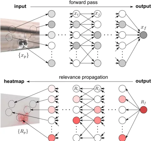
divide-and-conquer paradigm, and exploits the property that the function learned by a deep network is decomposed into a set of simpler subfunctions, either enforced structurally by the neural network connectivity, or occurring as a result of training. These subfunctions can, for example, apply locally to subsets of pixels, or they can operate at a certain level of abstraction based on the layer at which they are located in the deep network. An example of neural network mapping an input image to some score indicating the presence of an object of a certain class is given inFig. 2(top).
Let us assume that the functionf( )x encoded by the output neuron
xfhas been decomposed on the set of neurons at a given layer. Letxjbe
one such neuron andRjbe its associated relevance. We would like to
decompose Rj on the set of lower layer neurons{ }xi to whichxj is
connected. Assuming that{ }xi andRjare related by a functionRj({ })xi ,
such decomposition onto input neurons can be obtained by Taylor decomposition. It should be noted, however, that the relevance function may in practice depend on additional variables in the neural network, for example, the relevances of upper-layer neurons{ }xk to
which xj contributes. These top-down dependencies include the
necessary information to determine whether a neuron xjis relevant,
not only based on the pattern it receives as input, but also based on its context. For now, we will take for granted, that these top-down dependencies in the relevance function are such, that one can always decomposeRjexclusively in terms of{ }xi . Practical relevance models
that satisfy this property will be introduced inSection 5.
We define a root point{ }x∼i( )j of this function. Note that we choose a
different root point for each neuronxjin the current layer, hence the
superscript( )j to identify them. The Taylor decomposition ofR jis given by: ⎛ ⎝ ⎜ ⎞⎠⎟
∑
R R x x x ε R x x x ε = ∂ ∂{ } ·({ } − { } ) + = ∂ ∂ ·( − ) + , ∼ ∼ j j i x i i j j i j i x i i j R j { } ⊤ ( ) { } ( ) ∼i j ∼ i j ij ( ) ( )whereεjdenotes the Taylor residual, and where{ }x∼i( )j indicates that the derivative has been evaluated at the root point{ }x∼i( )j. The identified
termRijis the redistributed relevance from neuronxjto neuronxiin
the lower layer. To determine the total relevance of neuron xi, one
needs to pool relevance coming from all neurons{ }xj to which the
neuronxicontributes:
∑
Ri= R .j ij
Combining the last two equations, we get
∑
R R x x x = ∂ ∂ ·( − ). ∼ i j j i x i i j { } ( ) ∼i( )j (6) This last equation will be central for computing explicit relevance redistribution formulas based on specific choices of root points{ }x∼i( )j.It can be verified from the equations above that if∀ : ∑j iRij=Rj, in
particular, when all residuals εj are zero, then ∑iRi= ∑jRj, i.e. the
propagation from one layer to another is conservative in the sense of Definition 1. Moreover, if each layer-wise Taylor decomposition in the network is conservative, then, the chain of equalities Rf=…= ∑jRj= ∑iRi=…= ∑pRp holds, and the global pixel-wise
de-composition is thus also conservative. This chain of equalities is referred by[25]as layer-wise relevance conservation. Similarly, if Definition 2 holds for each local Taylor decomposition, the positivity of relevance scores at each layerRf, …, { }, { }, …, {Rj Ri Rp} ≥ 0is also ensured. If all Fig. 1.Difference between sensitivity analysis and decomposition for an exemplary two-dimensional functionf( )x. The function value is represented with contour lines. Explanations are represented as a vectorfield.
local Taylor decompositions are consistent in the sense ofDefinition 3, then, the whole decomposition is consistent in the same sense.
Fig. 2illustrates the procedure of layer-wise relevance propagation on a cartoon example where an image of a cat is presented to a deep network. If the neural network has been designed and trained successfully for the detection task, it is likely to have a structure, where neurons are modeling specific features at distinct locations. In such network, relevance redis-tribution is not only easier in the top layer where it has to be decided which neurons, and not pixels, are relevant for the object“cat”. It is also easier in the lower layers where the relevance has already been redis-tributed to the relevant neurons, and where thefinal redistribution step only involves a few neighboring pixels.
4. Application to one-layer networks
As a starting point for better understanding deep Taylor decom-position, in particular, how it leads to practical propagation rules, we work through a simple example, with advantageous analytical proper-ties. We consider a detection-pooling network made of one layer of nonlinearity. The network is defined as
⎛ ⎝ ⎜⎜ ⎞ ⎠ ⎟⎟
∑
∑
xj= max 0, x w +b and x = x i i ij j k j j (7) where{ }xi is ad-dimensional input,{ }xj is a detection layer,xkis theoutput, and θ= {wij,bj}are the weight and bias parameters of the network. The one-layer network is depicted inFig. 3.
The mapping{ } →xi xkdefines a functiong∈., where.denotes the
set of functions representable by this one-layer network. We will set an additional constraint on biases, where we forcebj≤ 0for allj. Imposing this constraint guarantees the existence of a root point{ }x∼i of the function
g (located at the origin), and thus also ensures the applicability of standard Taylor decomposition, for which a root point is needed. We
now perform the deep Taylor decomposition of this function. We start by equating the predicted output to the amount of total relevance that must be backpropagated, i.e.,Rk=xk. The relevance for the top layer can now be
expressed in terms of lower-layer neurons as:
∑
Rk= x
j j
(8) Having established the mapping between{ }xj andRk, we would like to
redistributeRkonto neurons{ }xj . Using Taylor decomposition (Eq.(4)),
redistributed relevancesRjcan be written as:
R R x x x = ∂ ∂ ·( − ). ∼ j k j x j j { }∼j (9) We still need to choose a root point{ }x∼j . The list of all root points of this
function is given by the plane equation∑jx∼j= 0. However, for the root to play its role of reference point, it should be admissible. Here, because of the application of the functionmax(0, ·)in the preceding layer, the root point must be positive. The only point that is both a root (∑jx∼j= 0) and admissible (∀ :j x∼j≥ 0) is{ } =x∼j 0. Choosing this root point in Eq.(9), and
Fig. 2.Computationalflow of deep Taylor decomposition. A prediction for the class“cat”is obtained by forward-propagation of the pixel values{ }xp, and is encoded by the output neuronxf. The output neuron is assigned a relevance scoreRf=xfrepresenting the total evidence for the class“cat”. Relevance is then backpropagated from the top layer down to the
input, where{Rp}denotes the pixel-wise relevance scores, that can be visualized as a heatmap.
Fig. 3.Detection-pooling network that implements Eqs.(7): thefirst layer detects features in the input space, the second layer pools the detected features into an output score.
observing that the derivative∂Rx = 1
∂
k
j , we obtain thefirst rule for relevance redistribution:
Rj=xj (10)
In other words, the relevance must be redistributed on the neurons of the detection layer in same proportion as their activation value. Trivially, we can also verify that the relevance is conserved during the redistribution process (∑jRj= ∑jxj=Rk) and positive (Rj=xj≥ 0). Let us now
express the relevance Rj as a function of the input neurons { }xi .
Because Rj=xjas a result of applying the propagation rule of Eq.(10),
we can write ⎛ ⎝ ⎜⎜ ⎞ ⎠ ⎟⎟
∑
Rj= max 0, x w +b , i i ij j (11) that establishes a mapping between{ }xi andRj. To obtain redistributedrelevances{ }Ri , we will apply Taylor decomposition again on this new
function. The identification of the redistributed total relevance∑jRjonto
the preceding layer was identified in Eq.(6)as:
∑
R R x x x = ∂ ∂ ·( − ). ∼ i j j i x i i j { } ( ) ∼i( )j (12) Relevances{ }Ri can therefore be obtained by performing as many Taylordecompositions as there are neurons in the hidden layer. We will introduce below various methods for choosing a root{ }x∼i( )j that consider
the diversity of possible input domains?⊆dto which the data belongs.
Each choice of input domain and associated method tofind a root will lead to a different rule for propagating relevance{ }Rj to{ }Ri .
4.1. Unconstrained input space and thew2-rule
Wefirst consider the simplest case where any real-valued input is admissible (?=d). In that case, we can always choose the root point
x
{ }∼i( )j that is nearest in the Euclidean sense to the actual data point{ }xi .
When Rj > 0, the nearest root of Rj as defined in Eq. (11) is the
intersection of the plane equation∑ix∼i w +b = 0
j
ij j
( ) , and the line of
maximum descent{ }x∼i( )j = { } + ·xi twj, wherewj is the vector of weight
parameters that connects the input to neuron xj and t∈. The
intersection of these two subspaces is the nearest root point. It is given by{ }x∼i j = {xi− ( ∑x w +b)} w w i i ij j ( ) ∑ ij i ij2
. Injecting this root into Eq.(12), the redistributed relevance becomes:
∑
R w w R = ∑ i j ij i i j j 2 ′ 2′ (13)The propagation rule consists of redistributing relevance according to the square magnitude of the weights, and pooling relevance across all neuronsj. This rule is also valid forRj=0, where the actual point{ }xi is
already a root, and for which no relevance needs to be propagated. Proposition 1.For allg∈.,the deep Taylor decomposition with the w2-rule is consistent in the sense of Definition3.
The w2-rule resembles the rule by[46,44] for determining the
importance of input variables in neural networks, where absolute values ofwijare used in place of squared values. It is important to
note that the decomposition that we propose here is modulated by the upper layer data-dependentRjs, which leads to an individual
explana-tion for each data point.
4.2. Constrained input space and thez-rules
When the input domain is restricted to a subset?⊂d, the nearest
root ofRjin the Euclidean sense might fall outside of?. Finding the
nearest root in this constrained input space can be difficult. An alternative is to further restrict the search domain to a subset of? where nearest root search becomes feasible again. Wefirst study the
case?=d+, which arises, for example in feature spaces that follow the
application of rectified linear units. In that case, we restrict the search domain to the segment({ 1xi wij< 0}, { }) ⊂xi d+, that we know contains
at least one root. The relevance propagation rule then becomes:
∑
R z z R = ∑ i j ij i i j j + ′ +′(calledz+-rule), where z =x w
ij+ i ij+, and wherewij+denotes the positive
part of wij. This rule corresponds for positive input spaces to the
αβ-rule proposed by[25]withα= 1andβ= 0. Thez+-rule will be used
in Section 5 to propagate relevances in higher layers of a neural network where neuron activations are positive.
Proposition 2.For all g∈. and data points{ } ∈xi d+, the deep
Taylor decomposition with thez+ -rule is consistent in the sense of
Definition3.
For image classification tasks, pixel spaces are typically subjects to box-constraints, where an image has to be in the domain
x l x h
= {{ }: ∀i i ≤ ≤ }
d
i i i
=1
) , whereli≤ 0 and hi≥ 0 are the smallest
and largest admissible pixel values for each dimension. In that new constrained setting, we can restrict the search for a root on the segment
l h x
({ 1i wij> 0+ i w1ij< 0}, { }) ⊂i ), where we know that there is at least
one root at itsfirst extremity. Finding the nearest root on that segment and injecting it into Eq.(12), we obtain the relevance propagation rule:
∑
R z l w h w z l w h w R = − − ∑ − − i j ij i ij i ij i i j i i j i i j j + − ′ ′ +′ −′(calledz)-rule), wherezij=x wi ij, and where we note the presence of
data-independent additive terms in the numerator and denominator. The idea of using an additive term in the denominator was formerly proposed by[25]and calledϵ-stabilized rule. However, the objective of [25] was to make the denominator non-zero to avoid numerical instability, while in our case, the additive terms serve to enforce positivity.
Proposition 3.For all g∈. and data points{ } ∈xi ), the deep
Taylor decomposition with thez) -rule is consistent in the sense of Definition3.
Detailed derivations of the proposed rules, proofs ofPropositions 1–3, and algorithms that implement these rules efficiently are given in the supplement.
5. Application to deep networks
In order to represent efficiently complex hierarchical problems, one needs deeper architectures. These architectures are typically made of several layers of nonlinearity, where each layer extracts features at different scale. An example of deep architecture is shown inFig. 4(left). In this example, the input is first processed by feature extractors localized in the pixel space. The resulting features are combined into more complex mid-level features that cover more pixels. Finally, these more complex features are combined in a final stage of nonlinear mapping, that produces a score determining whether the object to detect is present in the input image or not. A practical example of deep network with similar hierarchical architecture, and that is frequently used for image recognition tasks, is the convolutional neural network [47]. InSection 3, we have assumed the existence and knowledge of a functional mapping between the neuron activities at a given layer and relevances in the higher layer. This was the case for the small network ofSection 4. However, in deeper architectures, the mapping may be unknown (although it may still exist). In order to redistribute the relevance from higher to lower layers, one needs to make this mapping explicit. For this purpose, we introduce the concept of relevance model. A relevance model is a function that maps a set of neuron activations at a given layer to the relevance of a neuron in a higher layer, and whose output can be redistributed onto its input variables,
for the purpose of propagating relevance backwards in the network. For the deep network ofFig. 4(left), on can for example, try to predictRk
from{ }xi , which then allows us to decompose the predicted relevance
Rk into lower-layer relevances{ }Ri . The relevance models we will
consider borrow the structure of the one-layer network studied in Section 4, and for which we have already derived a deep Taylor decomposition.
Upper-layer relevance is not only determined by input neuron activations of the considered layer, but also by high-level information (i.e. abstractions) that have been formed in the top layers of the network. These high-level abstractions are necessary to ensure a global cohesion between low-level parts of the heatmap.
5.1. Min–max relevance model
Wefirst consider a trainable relevance model ofRk. This relevance
model is illustrated inFig. 4(top right) and is designed to incorporate both bottom-up and top-down information, in a way that the relevance can still be fully decomposed in terms of input neurons. It is defined as
⎛ ⎝ ⎜⎜ ⎞ ⎠ ⎟⎟
∑
∑
yj= max 0, x v +a and R = y. i i ij j k j j lwhere aj= min(0, ∑lR vl lj+dj) is a negative bias that depends on upper-layer relevances, and where∑lruns over the detection neurons of that upper-layer. This negative bias plays the role of an inhibitor, in particular, it prevents the activation of the detection unit yj of the
relevance model in the case where no upper-level abstraction in{ }Rl
matches the feature detected in{ }xi .
The parameters{ ,vij vlj,dj}of the relevance model are learned by minimization of the mean square error objective
R R
min (lk− k) ,2
whereRkis the true relevance,Rlkis the predicted relevance, and〈·〉is
the expectation with respect to the data distribution. Because the relevance model has the same structure as the one-layer network described inSection 4, in particular, becauseajis negative and only
weakly dependent on the set of neurons{ }xi , one can apply the same set
of rules for relevance propagation. We compute
Rj=yj (14)
for the pooling layer and
∑
R q q R = ∑ i j ij i i j j ′ ′ (15)for the detection layer, where qij=vij2, qij=x vi ij+, or
qij=x vi ij−l vi ij+−h vi ij−if choosing the w2-,z+-,z)-rules respectively.
This set of equations used to backpropagate relevance fromRkto{ }Ri ,
is approximately conservative, with an approximation error that is determined by how much on average the output of the relevance model Rlkdiffers from the true relevanceRk.
5.2. Training-free relevance model
A large deep neural network may have taken weeks or months to train, and we should be able to explain it without having to train a relevance model for each neuron. We consider the original feature extractor ⎛ ⎝ ⎜⎜ ⎞ ⎠ ⎟⎟
∑
xj= max 0, x w +b and x = ∥{ }∥x i i ij j k j qwhere theLq-norm can represent a variety of pooling operations such
as sum-pooling or max-pooling. Assuming that the upper-layer has been explained by thez+-rule, and indexing bylthe detection neurons
of that upper-layer, we can write the relevanceRkas
∑
R x w x w R = ∑ . k l k kl k k k l l + ′ ′ +′Taking xk out of the sum, and using the identity∑jxj= ∥{ }∥xj 1for
xj≥ 0, we can rewrite the relevance as
⎛ ⎝ ⎜ ⎜ ⎞ ⎠ ⎟ ⎟
∑
Rk= x · ·c d j j k k whereck= x x ∥ { } ∥ ∥ { } ∥ j q j 1 is a Lq/L1pooling ratio, andd = ∑
k l w R x w ∑ kl l k k k l + ′ ′ +′ is a top-down contextualization term. Modeling the terms ck anddk as
constant under a perturbation of the activities{ }xj , we obtain the “training-free”relevance model, that we illustrate in Fig. 4 (bottom right). We give below some arguments that support the modeling ofck
anddkas constants.
First, we can observe that ck is indeed constant under certain
transformations such as a homogeneous rescaling of the activations x
{ }j , or any permutation of neurons activations within the pool. More
generally, if we consider a sufficiently large pool of neurons { }xj ,
independent variations of individual neuron activations within the pool can be viewed as swapping activations between neurons without changing the actual value of these activations. These repeated swaps also keep the norms and their ratio constant. For the top-down term
dk, we remark that the most direct way it is influenced by{ }xj is
through the variablexk′ of the sum in the denominator ofdk, when
k′ =k. As the sum combines many neuron activations, the effect of{ }xj
ondkcan also be expected to be very limited. Modelingckanddkas
constants enables us to backpropagate the relevance on the lower layers: Because the relevance modelRkabove has the same structure as
the network ofSection 4(up to a constant factorc dk k), it is easy to
Fig. 4.Left: Example of a 3-layer deep network, composed of increasingly high-level feature extractors. Right: Diagram of the two proposed relevance models for redistributing relevance onto lower layers.
derive its Taylor decomposition, in particular, we obtain the rules R x x R = ∑ , j j j j k ′ ′
where relevance is redistributed in proportion to activations in the detection layer, and
∑
R q q R = ∑ , i j ij i i j j ′ ′ whereqij=wij2,qij=x wi ij+, orqij=x wi ij−l wi ij+−h wi ij−, corresponding tothew2-,z+-,z)-rules respectively. If we choose thez+-rule for that layer
again, the same training-free decomposition technique can be applied to the layer below, and the process can be repeated until the input layer. Thus, when using the training-free relevance model, all layers of the network must be decomposed using thez+-rule, except for thefirst
layer to which other rules can be applied such as thew2-rule or the
z)-rule.
6. Experiments
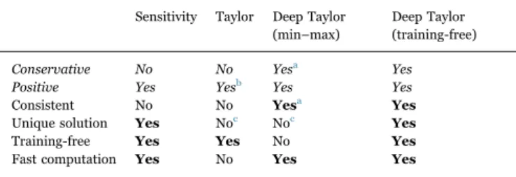
In this section, we would like to test how well deep Taylor decomposition performs empirically, in particular, if the resulting heatmaps are able to pinpoint the relevant information in the input data. Wefirst consider a neural network composed of two detection-pooling layers applied on a simple MNIST-based task. Then, we test our method on large convolutional neural networks for general image classification.Table 1lists the main technical properties of the various methods used in the experiments.
6.1. Experiment on MNIST
The MNIST dataset consists of 60 000 training and 10 000 test images of size 28×28 representing handwritten digits, along with their label (from 0 to 9). We consider an artificial problem consisting of detecting the presence of a digit with label 0–3 in an image of size 28×56 built as a concatenation of two MNIST digits. There is a virtually infinite number of possible combinations.
A neural network with 28×56 input neurons and one output neuron is trained on this task. The input values are coded between−0.5(black) and+1.5(white). The neural network is composed of afirst detection-pooling layer with 400 detection neurons sum-pooled into 100 units (i.e. we sum-pool non-overlapping groups of 4 detection units). A second detection-pooling layer with 400 detection neurons is applied to the 100-dimensional output of the previous layer, and activities are sum-pooled onto a single unit representing the deep network output. Positive examples are assigned target value 100 and negative examples are assigned target value 0. The neural network is trained to minimize the mean-square error between the target values and its output xf.
Treating the supervised task as a regression problem forces the
network to assign approximately the same amount of relevance to all positive examples, and as little relevance as possible to the negative ones. Weights of the network are initialized using a normal distribution of mean 0 and standard deviation 0.05. Biases are initialized to zero and constrained to be negative or zero throughout training. Training data is extended with translated versions of MNIST digits. The deep network is trained using stochastic gradient descent with minibatch size 20, for 300 000 iterations, and using a small learning rate.
We compare four heatmapping techniques: sensitivity analysis, stan-dard Taylor decomposition, and the min-max and training-free variants of deep Taylor decomposition. Sensitivity analysis is straightforward to apply. For standard Taylor decomposition, the root x∼ is chosen to be the nearest point such that f( ) < 0.1 ( )x∼ f x. For the deep Taylor decom-position models, we apply thez+-rule in the top layer and thez)-rule in
thefirst layer. Thez)-rule is computed using as lower- and upper-bounds lp= −0.5andhp=1.5. For the min-max variant, the relevance model in
thefirst layer is trained to minimize the mean-square error between the relevance model output and the true relevance (obtained by application of thez+-rule in the top layer). It is trained in parallel to the actual neural
network, using similar training parameters.
Fig. 5shows the analysis for 12 positive examples generated from the MNIST test set and processed by the deep neural network. Heatmaps are shown below their corresponding example for each heatmapping method. In all cases, we can observe that the heatmap-ping procedure correctly assigns most of the relevance to pixels where the digit to detect is located, and ignores the distracting digit.
Sensitivity analysis produces unbalanced and incomplete heatmaps, with some examples reacting strongly, and others weakly. There is also a non-negligible amount of relevance allocated to the border of the image (where there is no information), or placed on the distractor digit. Nearest root Taylor decomposition ignores irrelevant pixels in the background but is still producing spurious relevance on the distractor digit. On the other hand, deep Taylor decomposition produces rele-vance maps that are less affected by the distractor digit and that are also better balanced spatially. The heatmaps obtained by the trained min-max model and the training-free method are of similar quality, suggesting that the approximations made inSection 5.2are also valid empirically.
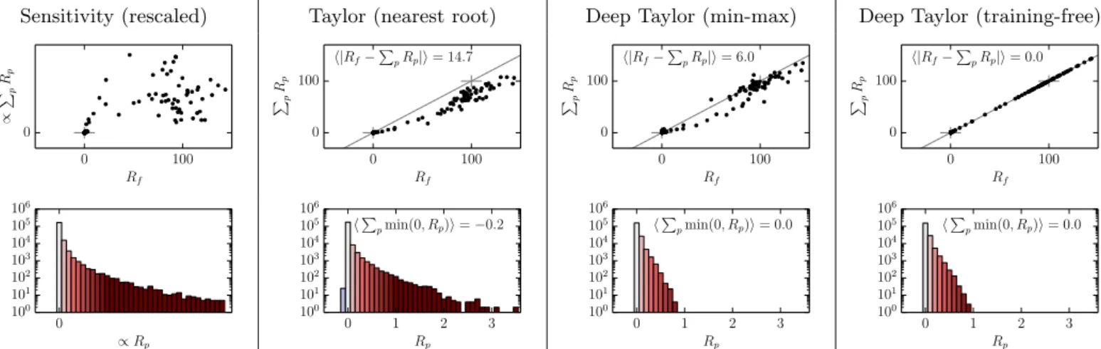
Fig. 6 quantitatively evaluates the heatmapping techniques of Fig. 5. The scatter plots compare the total output relevance with the sum of pixel-wise relevances. Each point in the scatter plot is a different example drawn independently from the input distribution. These scatter plots test empirically for each heatmapping method whether it is conservative in the sense ofDefinition 1. In particular, if all points lie on the diagonal line of the scatter plot, then ∑pRp=Rf, and the
heatmapping is conservative. The histograms just below test empiri-cally whether the studied heatmapping methods satisfy positivity in the sense ofDefinition 2, by counting the number of times (shown on a log-scale) pixel-wise contributionsRptake a certain value. Red color in the
histogram indicates positive relevance assignments, and blue color indicates negative relevance assignments. Therefore, an absence of blue bars in the histogram indicates that the heatmap is positive (the desired behavior). Overall, the scatter plots and the histograms produce a complete description of the degree of consistency of the heatmapping techniques in the sense ofDefinition 3.
Sensitivity analysis only measures a local effect and therefore does not conceptually redistribute relevance onto the input. However, we can still measure the relative strength of computed sensitivities between examples or pixels. The nearest root Taylor decomposition is positive, but dissipates relevance. The deep Taylor decomposition with the min-max relevance model produces near-conservative heatmaps, and the training-free deep Taylor decomposition produces heatmaps that are fully conservative. Deep Taylor decomposition spreads rele-vance onto more pixels than competing methods, as shown by the shorter tail of its relevance histogram. Both deep Taylor decomposition variants shown here also ensures positivity, due to the application of Table 1
Summary of the technical properties of neural network heatmapping methods described in this paper.
Sensitivity Taylor Deep Taylor (min–max)
Deep Taylor (training-free) Conservative No No Yesa Yes
Positive Yes Yesb Yes Yes
Consistent No No Yesa Yes
Unique solution Yes Noc Noc Yes
Training-free Yes Yes No Yes
Fast computation Yes No Yes Yes
aup to afitting error between the redistributed relevance and the relevance model output.
busing the differentiable approximationmax(0, ) = limx t log(0.5 + 0.5 exp( ))tx
t→∞−1 .
thez)- andz+-rule in the respective layers.
6.2. Experiment on ILSVRC
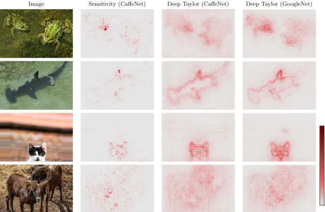
We now apply the fast training-free deep Taylor decomposition to explain decisions made by large neural networks (BVLC Reference CaffeNet [48] and GoogleNet [12]) trained on the dataset of the ImageNet large scale visual recognition challenges ILSVRC 2012[49] and ILSVRC 2014 [50] respectively. We keep the neural networks unchanged. We compare our decomposition method to sensitivity analysis. Both methods perform a single backward pass in the network and are therefore suitable for analyzing the predictions of these highly complex models.
The methods are tested on a number of images from Pixabay.com and Wikimedia Commons. Thez)-rule is applied to thefirst
convolu-tion layer. For all higher convoluconvolu-tion and fully-connected layers, the z+-rule is applied. Positive biases (that are not allowed in our deep
Taylor framework) are treated as neurons, on which relevance can be redistributed (i.e. we add max(0,bj) in the denominator of z)- and z+-rules). Normalization layers are bypassed in the relevance
propaga-tion pass. In order to visualize the heatmaps in the pixel space, we sum the relevances of the three color channels, leading to single-channel heatmaps, where the red color designates relevant regions.
Fig. 7shows the heatmaps resulting from deep Taylor decomposi-tion for four different images. For example, heatmaps identify as relevant the dorsal fin of the shark and the head of the cat. The heatmaps can detect two instances of the same object within a single image, here, the two frogs. The heatmaps also ignore most of the distracting structure, such as the horizontal lines above the cat's head.
Sometimes, the object to detect is shown in a less stereotypical pose or is hard to separate from the background. For example, the sheeps are overlapping and are superposed to a background of same color, leading to a more diffuse heatmap.
Sensitivity analysis ignores or overrepresents some of the relevant regions. For example, the leftmost frog in thefirst image is assigned more importance than the second frog. Some of the contour of the shark in the second image is ignored. On the other hand, deep Taylor decomposition produces heatmaps that cover the explanatory features in a more comprehensive manner and also better match the saliency of the objects to detect in the input image. See[27] for a quantitative comparison of sensitivity analysis and relevance propagation methods similar to deep Taylor decomposition on this data.
Decompositions for CaffeNet and GoogleNet predictions have a high level of similarity. It demonstrates a certain level of transparency of the method to the choice of deep network architecture supporting the prediction. We can however observe that GoogleNet heatmaps are of higher quality, in particular, with better spatial resolution, and the ability to detect relevant features even in cluttered scenes such as the last image, where the characteristic v-shaped nose of the sheep is still identified as relevant. Instead, AlexNet is more reliant on context for its predictions, and uses more pixels to detect contours of the relevant objects. The observation that more accurate predictions are supported by better resolved input patterns is also in line with other studies [51,52].
Fig. 8studies the special case of an image of class“volcano”, and a zoomed portion of it. On a global scale, the heatmapping method recognizes the characteristic outline of the volcano. On a local scale, the relevance is present on both sides of the edge of the volcano, which is Fig. 5.Comparison of heatmaps produced by various decompositions and relevance models. Each input image is presented with its associated heatmap.
Fig. 6.Top: Scatter plots showing for each type of decomposition and data points the predicted class score (x-axis), and the sum-of-relevance in the input layer (y-axis).Bottom: Histograms showing the number of times (on a log-scale) a particular pixel-wise relevance score occurs.
consistent with the fact that the two sides of the edge are necessary to detect it. The zoomed portion of the image also reveals different stride sizes in the first convolution layer between CaffeNet (stride 4) and GoogleNet (stride 2). Observation of these global and local character-istics of the heatmap provides a visual feedback of the way relevance
flows in the deep network.
7. Conclusion
Nonlinear machine learning models have become standard tools in science and industry due to their excellent performance even for large, complex and high-dimensional problems. However, in practice it becomes more and more important to understand the underlying nonlinear model, i.e., to achieve transparency of whataspect of the input makes the model decide. To achieve this, we have contributed by novel conceptual ideas to deconstruct nonlinear models. Specifically, we have proposed a novel approach to relevance propagation called deep Taylor decomposition, and used it to assess the importance of single pixels in image classification tasks. We were able to compute
heatmapsthat clearly and intuitively allow to better understand the role of input pixels when classifying an unseen data point. We have shed light on theoretical connections between the Taylor decomposi-tion of a funcdecomposi-tion, and rule-based relevance propagadecomposi-tion techniques, showing a clear relationship between the two approaches for a particular class of neural networks. We have introduced the concept of relevance model as a mean to scale the analysis to networks with many layers. Our method is stable under different architectures and datasets, and does not require hyperparameter tuning. We would like to stress, that we are free to use as a starting point of our framework either an own trained and carefully tuned neural network model or we may also download existing pre-trained deep network models (e.g. the BVLC CaffeNet[48]) that have already been shown to achieve excellent performance on benchmarks. In both cases, our method provides explanation. In other words our approach is orthogonal to the quest for enhanced results on benchmarks, in fact, we can use any bench-mark winner and then enhance its transparency to the user.
Acknowledgments
This work was supported by the Brain Korea 21 Plus Program through the National Research Foundation of Korea; the Deutsche Forschungsgemeinschaft (DFG) [grant MU 987/17-1]; a SUTD Start-Fig. 7.Images of different ILSVRC classes (“frog”,“shark”,“cat”, and“sheep”) given as input to a deep network, and displayed next to the corresponding heatmaps. Heatmap scores are summed over all color channels of the image.
Fig. 8.Image with ILSVRC class“volcano”, displayed next to its associated heatmaps and a zoom on a region of interest.
Up Grant; and the German Ministry for Education and Research as Berlin Big Data Center (BBDC) [01IS14013A]. This publication only reflects the authors views. Funding agencies are not liable for any use that may be made of the information contained herein.
Appendix A. Supplementary data
Supplementary data associated with this article can be found in the online version athttp://dx.doi.org/10.1016/j.patcog.2016.11.008. References
[1]M.I. Jordan, Learning in Graphical Models, MIT Press, Cambridge, MA, USA, 1998.
[2]B. Schölkopf, A.J. Smola, Learning with Kernels Support Vector Machines, Regularization, Optimization, and Beyond, MIT Press, Cambridge, MA, USA, 2002. [3]K.-R. Müller, S. Mika, G. Rätsch, K. Tsuda, B. Schölkopf, An introduction to
kernel-based learning algorithms, IEEE Trans. Neural Netw. 12 (2) (2001) 181–201. [4]C.E. Rasmussen, C.K.I. Williams, Gaussian Processes for Machine Learning, MIT
Press, Cambridge, MA, USA, 2006.
[5]C.M. Bishop, Neural Networks for Pattern Recognition, Oxford University Press, Inc., New York, NY, USA, 1995.
[6] G. Montavon, G.B. Orr, K.-R. Müller (eds.), Neural Networks: Tricks of the Trade, Lecture Notes in Computer Science, vol. 7700. Springer, Berlin Heidelberg, 2012. [7] Y. LeCun, L. Bottou, G.B. Orr, K.-R. Müller, Efficient backprop, in: Neural
Networks: Tricks of the Trade, 2nd ed., Springer, Berlin Heidelberg, 2012, pp. 9– 48.
[8]R.E. Schapire, Y. Freund, Boosting, MIT Press, Cambridge, MA, USA, 2012. [9]L. Breiman, Random forests, Mach. Learn. 45 (1) (2001) 5–32.
[10] A. Krizhevsky, I. Sutskever, G.E. Hinton, Imagenet classification with deep convolutional neural networks, in: Advances in Neural Information Processing Systems, vol. 25, 2012, pp. 1106–1114.
[11] D.C. Ciresan, A. Giusti, L.M. Gambardella, J. Schmidhuber, Deep neural networks segment neuronal membranes in electron microscopy images, in: Advances in Neural Information Processing Systems, vol. 25, 2012, pp. 2852–2860. [12] C. Szegedy, W. Liu, Y. Jia, P. Sermanet, S.E. Reed, D. Anguelov, D. Erhan, V.
Vanhoucke, A. Rabinovich, Going deeper with convolutions, in: IEEE Conference on Computer Vision and Pattern Recognition, CVPR 2015, Boston, MA, USA, June 7–12, 2015, 2015, pp. 1–9.
[13] R. Collobert, J. Weston, L. Bottou, M. Karlen, K. Kavukcuoglu, P.P. Kuksa, Natural language processing (almost) from scratch, J. Mach. Learn. Res. 12 (2011) 2493–2537.
[14] R. Socher, A. Perelygin, J. Wu, J. Chuang, C.D. Manning, A. Ng, C. Potts, Recursive deep models for semantic compositionality over a sentiment treebank, in: Proceedings of the 2013 Conference on Empirical Methods in Natural Language Processing, Association for Computational Linguistics, October 2013, pp. 1631– 1642.
[15] S. Ji, W. Xu, M. Yang, K. Yu, 3d convolutional neural networks for human action recognition, in: Proceedings of the 27th International Conference on Machine Learning (ICML-10), June 21–24, 2010, Haifa, Israel, 2010, pp. 495–502. [16] Q.V. Le, W.Y. Zou, S.Y. Yeung, A.Y. Ng, Learning hierarchical invariant
spatio-temporal features for action recognition with independent subspace analysis, in: The 24th IEEE Conference on Computer Vision and Pattern Recognition, pp. 3361–3368, 2011.
[17] E.P. Ijjina, K.M. Chalavadi, Human action recognition using genetic algorithms and convolutional neural networks, Pattern Recognit. (2016).
[18] G. Montavon, M. Rupp, V. Gobre, A. Vazquez-Mayagoitia, K. Hansen, A. Tkatchenko, K.-R. Müller, O.A. von Lilienfeld, Machine learning of molecular electronic properties in chemical compound space, New J. Phys. 15 (9) (2013) 095003.
[19] P. Baldi, P. Sadowski, D. Whiteson, Searching for exotic particles in high-energy physics with deep learning, Nat. Commun. 5 (4308) (2014).
[20] S. Haufe, F.C. Meinecke, K. Görgen, S. Dähne, J. Haynes, B. Blankertz, F. Bießmann, On the interpretation of weight vectors of linear models in multi-variate neuroimaging, NeuroImage 87 (2014) 96–110.
[21] R. Oaxaca, Male-female wage differentials in urban labor markets, Int. Econ. Rev. 14 (3) (1973) 693–709.
[22] B. Poulin, R. Eisner, D. Szafron, P. Lu, R. Greiner, D.S. Wishart, A. Fyshe, B. Pearcy, C. Macdonell, J. Anvik, Visual explanation of evidence with additive classifiers, in: Proceedings, The Twenty-First National Conference on Artificial Intelligence and the Eighteenth Innovative Applications of Artificial Intelligence Conference, 2006, pp. 1822–1829.
[23] K. Simonyan, A. Vedaldi, A. Zisserman, Deep inside convolutional networks: visualising image classification models and saliency maps, CoRR (2013) vol. abs/ 1312.6034.
[24] M.D. Zeiler, R. Fergus, Visualizing and understanding convolutional networks, in: Computer Vision–ECCV 2014–13th European Conference, 2014, pp. 818–833. [25] S. Bach, A. Binder, G. Montavon, F. Klauschen, K.-R. Müller, W. Samek, On
pixel-wise explanations for non-linear classifier decisions by layer-pixel-wise relevance propagation, PLoS One 10 (7) (2015) e0130140.
[26] D. Rumelhart, G. Hinton, R. Williams, Learning representations by back-propa-gating errors, Nature 323 (6088) (1986) 533–536.
[27] W. Samek, A. Binder, G. Montavon, S. Lapuschkin, K.-R. Müller, Evaluating the visualization of what a deep neural network has learned, IEEE Trans. Neural Netw. Learn. Syst. 99 (2016) 1–14.
[28] M.L. Braun, J.M. Buhmann, K.-R. Müller, On relevant dimensions in kernel feature spaces, J. Mach. Learn. Res. 9 (2008) 1875–1908.
[29] G. Montavon, M.L. Braun, T. Krueger, K.-R. Müller, Analyzing local structure in kernel-based learning: explanation, complexity, and reliability assessment, IEEE Signal Process. Mag. 30 (4) (2013) 62–74.
[30] G. Montavon, M.L. Braun, K.-R. Müller, Kernel analysis of deep networks, J. Mach. Learn. Res. 12 (2011) 2563–2581.
[31] I.J. Goodfellow, Q.V. Le, A.M. Saxe, H. Lee, A.Y. Ng, Measuring invariances in deep networks, in: Advances in Neural Information Processing Systems, vol. 22, pp. 646–654, 2009.
[32] D. Erhan, A. Courville, Y. Bengio, Understanding Representations Learned in Deep Architectures, Technical Report 1355, University of Montreal, 2010.
[33] R. Krishnan, G. Sivakumar, P. Bhattacharya, Extracting decision trees from trained neural networks, Pattern Recognit. 32 (12) (1999) 1999–2009.
[34] R. Krishnan, G. Sivakumar, P. Bhattacharya, A search technique for rule extraction from trained neural networks, Pattern Recognit. Lett. 20 (3) (1999) 273–280. [35] D. Baehrens, T. Schroeter, S. Harmeling, M. Kawanabe, K. Hansen, K.-R. Müller,
How to explain individual classification decisions, J. Mach. Learn. Res. 11 (2010) 1803–1831.
[36] W. Landecker, M.D. Thomure, L.M.A. Bettencourt, M. Mitchell, G.T. Kenyon, S.P. Brumby, Interpreting individual classifications of hierarchical networks, in: IEEE Symposium on Computational Intelligence and Data Mining, 2013, pp. 32–38. [37] C. Szegedy, W. Zaremba, I. Sutskever, J. Bruna, D. Erhan, I.J. Goodfellow,
R. Fergus, Intriguing properties of neural networks, CoRR (2013) vol. abs/ 1312.6199.
[38] S. Bazen, X. Joutard, The Taylor decomposition: a unified generalization of the Oaxaca method to nonlinear models, Technical Report 2013-32, Aix-Marseille University, 2013.
[39] H. Fang, S. Gupta, F.N. Iandola, R.K. Srivastava, L. Deng, P. Dollár, J. Gao, X. He, M. Mitchell, J.C. Platt, C.L. Zitnick, G. Zweig, From captions to visual concepts and back, in: IEEE Conference on Computer Vision and Pattern Recognition, CVPR 2015, Boston, MA, USA, June 7–12, 2015, 2015, pp. 1473–1482.
[40] H. Larochelle, G.E. Hinton, Learning to combine foveal glimpses with a third-order Boltzmann machine, in: Advances in Neural Information Processing Systems 23, 2010, pp. 1243–1251.
[41] K. Xu, J. Ba, R. Kiros, K. Cho, A.C. Courville, R. Salakhutdinov, R.S. Zemel, Y. Bengio, Show, attend and tell: Neural image caption generation with visual attention, in: Proceedings of the 32nd International Conference on Machine Learning, 2015, pp. 2048–2057.
[42] L. Arras, F. Horn, G. Montavon, K.-R. Müller, W. Samek, Explaining predictions of non-linear classifiers in NLP, in: Proceedings of the Workshop on Representation Learning for NLP at Association for Computational Linguistics (ACL), 2016. [43] I. Sturm, S. Lapuschkin, W. Samek, K.-R. Müller, Interpretable deep neural
networks for single-trial EEG classification, J. Neurosci. Methods 274 (2016) 141–145.
[44] M. Gevrey, I. Dimopoulos, S. Lek, Review and comparison of methods to study the contribution of variables in artificial neural network models, Ecol. Model. 160 (3) (2003) 249–264.
[45] S. Moosavi-Dezfooli, A. Fawzi, P. Frossard, Deepfool: a simple and accurate method to fool deep neural networks, CoRR (2015) vol. abs/1511.04599.
[46] D.G. Garson, Interpreting neural-network connection weights, AI Expert 6 (4) (1991) 46–51.
[47] Y. LeCun, Generalization and network design strategies, in: Connectionism in Perspective, Elsevier, Zurich, Switzerland, 1989.
[48] Y. Jia, Caffe: an open source convolutional architecture for fast feature embedding, 2016,〈http://caffe.berkeleyvision.org〉.
[49] J. Deng, A. Berg, S. Satheesh, H. Su, A. Khosla, F.-F. Li, The ImageNet Large Scale Visual Recognition Challenge 2012 (ILSVRC2012)〈http://www.image-net.org/ challenges/LSVRC/2012〉.
[50] O. Russakovsky, J. Deng, H. Su, J. Krause, S. Satheesh, S. Ma, Z. Huang, A. Karpathy, A. Khosla, M.S. Bernstein, A.C. Berg, F. Li, Imagenet large scale visual recognition challenge, Int. J. Comput. Vis. 115 (3) (2015) 211–252.
[51] W. Yu, K. Yang, Y. Bai, H. Yao, Y. Rui, Visualizing and comparing convolutional neural networks, CoRR (2014) vol. abs/1412.6631.
[52] S. Lapuschkin, A. Binder, G. Montavon, K.-R. Müller, W. Samek, Analyzing classifiers: Fisher vectors and deep neural networks, in: IEEE Conference on Computer Vision and Pattern Recognition, 2016, pp. 2912–2920.
Grégoire Montavonreceived a Masters degree in Communication Systems from École Polytechnique Fédérale de Lausanne, in 2009 and a Ph.D. degree in Machine Learning from the Technische Universität Berlin, in 2013. He is currently a Research Associate in the Machine Learning Group at TU Berlin.
Sebastian Lapuschkinreceived a Masters degree in Computer Science from Technische Universität Berlin, in 2013. He currently is a Research Associate in the Machine Learning Group at the Fraunhofer Heinrich-Hertz-Institute while pursuing is Ph.D. at TU Berlin. His research interests are computer vision, machine learning and data analysis.
Alexander Binderis Assistant Professor at the Singapore University of Technology and Design. He received a Ph.D. in Machine Learning from Technische Universität Berlin, in 2013. He participated in Pascal VOC and ImageCLEF competitions before. His research interests include neural networks, image analysis and medical imaging.
Wojciech Samekreceived a Diploma degree in Computer Science from Humboldt University Berlin in 2010 and the Ph.D. degree in Machine Learning from Technische Universität Berlin, in 2014. Currently, he directs the Machine Learning Group at Fraunhofer Heinrich Hertz Institute. His research interests include neural networks and signal processing.
Klaus-Robert Müller(Ph.D. 92) has been a Professor of computer science at TU Berlin since 2006; co-director Berlin Big Data Center. He won the 1999 Olympus Prize of German Pattern Recognition Society, the 2006 SEL Alcatel Communication Award, and the 2014 Science Prize of Berlin. Since 2012, he is an elected member of the German National Academy of Sciences–Leopoldina.