Linear regression and ANOVA

(1)

Chapter 4

Linear regression and

ANOVA

Regression and analysis of variance (ANOVA) form the basis of many inves-tigations. In this chapter we describe how to undertake many common tasks in linear regression (broadly defined), while Chapter 5 discusses many general-izations, including other types of outcome variables, longitudinal and clustered analysis, and survival methods.

Many commands can perform linear regression, as it constitutes a special case of which many models are generalizations. We present detailed descriptions for thelm()command, as it offers the most flexibility and best output options tailored to linear regression in particular. While ANOVA can be viewed as a special case of linear regression, separate routines are available (aov()) to perform it. We address additional procedures only with respect to output that is difficult to obtain through the standard linear regression tools.

Many of the routines available return or operate onlmclass objects, which include coefficients, residuals, fitted values, weights, contrasts, model matrices, and the like (seehelp(lm)).

The CRAN Task View on Statistics for the Social Sciences provides an excellent overview of methods described here and in Chapter 5.

4.1

Model fitting

4.1.1

Linear regression

Example: See 4.7.3

mod1 = lm(y ~ x1 + ... + xk, data=ds) summary(mod1)

or

(2)

form = as.formula(y ~ x1 + ... + xk) mod1 = lm(form, data=ds)

summary(mod1)

The first argument of the lm() function is a formula object, with the out-come specified followed by the ∼ operator then the predictors. More in-formation about the linear model summary() command can be found using

help(summary.lm). By default, stars are used to annotate the output of the

summary()functions regarding significance levels: these can be turned off using the commandoptions(show.signif.stars=FALSE).

4.1.2

Linear regression with categorical covariates

Example: See 4.7.3 See also 4.1.3 (parameterization of categorical covariates)

x1f = as.factor(x1)

mod1 = lm(y ~ x1f + x2 + ... + xk, data=ds)

Theas.factor()command creates a categorical (or factor/class) variable from a variable. By default, the lowest value (either numerically or by ASCII char-acter code) is the reference value when a factor variable is in a formula. The

levels option for the factor() function can be used to select a particular reference value (see also 2.4.16).

4.1.3

Parameterization of categorical covariates

Example: See 4.7.6 In R,as.factor()can be applied before or within any model-fitting function. Parameterization of the covariate can be controlled as in the second example below.

mod1 = lm(y ~ as.factor(x))

or

x.factor = as.factor(x)

mod1 = lm(y ~ x.factor, contrasts=list(x.factor="contr.SAS"))

Theas.factor()function creates a factor object. Thecontrasts option for thelm()function specifies how the levels of that factor object should be coded. Thelevelsoption to thefactor()function allows specification of the ordering of levels (the default is alphabetical). An example can be found at the beginning of Section 4.7.

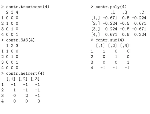
The specification of the design matrix for analysis of variance and regres-sion models can be controlled using the contrasts option. Examples of op-tions (for a factor with 4 equally spaced levels) are given in Table 4.1. See

options("contrasts")for defaults, andcontrasts()orlm()to apply a con-trast function to a factor variable. Support for reordering factors is available

(3)

4.1. MODEL FITTING 95

using thereorder()function. Ordered factors can be created using theordered()

function. > contr.treatment(4) > contr.poly(4) 2 3 4 .L .Q .C 1 0 0 0 [1,] -0.671 0.5 -0.224 2 1 0 0 [2,] -0.224 -0.5 0.671 3 0 1 0 [3,] 0.224 -0.5 -0.671 4 0 0 1 [4,] 0.671 0.5 0.224 > contr.SAS(4) > contr.sum(4) 1 2 3 [,1] [,2] [,3] 1 1 0 0 1 1 0 0 2 0 1 0 2 0 1 0 3 0 0 1 3 0 0 1 4 0 0 0 4 -1 -1 -1 > contr.helmert(4) [,1] [,2] [,3] 1 -1 -1 -1 2 1 -1 -1 3 0 2 -1 4 0 0 3

Table 4.1: Built-In Options for Contrasts

4.1.4

Linear regression with no intercept

mod1 = lm(y ~ 0 + x1 + ... + xk, data=ds)

or

mod1 = lm(y ~ x1 + ... + xk -1, data=ds)

4.1.5

Linear regression with interactions

Example: See 4.7.3

mod1 = lm(y ~ x1 + x2 + x1:x2 + x3 + ... + xk, data=ds)

or

lm(y ~ x1*x2 + x3 + ... + xk, data=ds)

The* operator includes all lower order terms, while the : operator includes only the specified interaction. So, for example, the commandsy ∼ x1*x2*x3

(4)

values. The syntax also works with any covariates designated as categorical using theas.factor() command (see 4.1.2).

4.1.6

Linear models stratified by each value of a grouping

variable

Example: See 4.7.5 See also 2.5.1 (subsetting) and 3.1.2 (summary measure by groups)

uniquevals = unique(z)

numunique = length(uniquevals)

formula = as.formula(y ~ x1 + ... + xk) p = length(coef(lm(formula)))

params = matrix(numeric(numunique*p), p, numunique) for (i in 1:length(uniquevals)) {

cat(i, "\n")

params[,i] = coef(lm(formula, subset=(z==uniquevals[i]))) }

or

modfits = by(ds, z, function(x) lm(y ~ x1 + ... + xk, data=x)) sapply(modfits, coef)

In the first codeblock, separate regressions are fit for each value of the grouping variablezthrough use of aforloop. This requires the creation of a matrix of resultsparamsto be set up in advance, of the appropriate dimension (number of rows equal to the number of parameters (p=k+1) for the model, and number of columns equal to the number of levels for the grouping variablez). Within the loop, thelm()function is called and the coefficients from each fit are saved in the appropriate column of theparamsmatrix.

The second code block solves the problem using the by() function, where thelm() function is called for each of the values forz. Additional support for this type ofsplit-apply-combine strategy is available inlibrary(plyr).

4.1.7

One-way analysis of variance

Example: See 4.7.6

xf = as.factor(x)

mod1 = aov(y ~ xf, data=ds) summary(mod1)

The summary() command can be used to provide details of the model fit. More information can be found usinghelp(summary.aov). Note that the func-tionsummary.lm(mod1) will display the regression parameters underlying the ANOVA model.

(5)

4.2. MODEL COMPARISON AND SELECTION 97

4.1.8

Two-way (or more) analysis of variance

Example: See 4.7.6 See also 4.1.5 (interactions) and 6.1.13 (interaction plots)

aov(y ~ as.factor(x1) + as.factor(x2), data=ds)

4.2

Model comparison and selection

4.2.1

Compare two models

Example: See 4.7.6

mod1 = lm(y ~ x1 + ... + xk, data=ds) mod2 = lm(y ~ x3 + ... + xk, data=ds) anova(mod2, mod1)

or

drop1(mod2)

Two nested models may be compared using theanova()function. Theanova()

command computes analysis of variance (or deviance) tables. When given one model as an argument, it displays the ANOVA table. When two (or more) nested models are given, it calculates the differences between them. The func-tion drop1() computes a table of changes in fit for each term in the named linear model object.

4.2.2

Log-likelihood

Example: See 4.7.6 See also 4.2.3 (AIC)

mod1 = lm(y ~ x1 + ... + xk, data=ds) logLik(mod1)

The logLik() function supports glm, lm, nls, Arima, gls, lme, and nlme

objects.

4.2.3

Akaike Information Criterion (AIC)

Example: See 4.7.6 See also 4.2.2 (log-likelihood)

mod1 = lm(y ~ x1 + ... + xk, data=ds) AIC(mod1)

TheAIC() function includes support for glm, lm, nls, Arima, gls, lme, and

nlmeobjects. The stepAIC()function withinlibrary(MASS)allows stepwise model selection using AIC (see also 5.4.4, LASSO).

(6)

4.2.4

Bayesian Information Criterion (BIC)

Joint null hypotheses: Sum of parameters

mod1 = lm(y ~ x1 + ... + xk, data=ds)

mod2 = lm(y ~ I(x1+x2-1) + ... + xk, data=ds) anova(mod2, mod1)

or

mod1 = lm(y ~ x1 + ... + xk, data=ds) covb = vcov(mod1)

coeff.mod1 = coef(mod1)

t = (coeff.mod1[2,1]+coeff.mod1[3,1]-1)/ sqrt(covb[2,2]+covb[3,3]+2*covb[2,3]) pvalue = 2*(1-pt(abs(t), mod1$df))

(7)

4.3. TESTS, CONTRASTS, AND LINEAR FUNCTIONS 99

TheI()function inhibits the interpretation of operators, to allow them to be used as arithmetic operators. The code in the lower example utilizes the same approach introduced in 4.3.1.

4.3.3

Tests of equality of parameters

Example: See 4.7.8

mod1 = lm(y ~ x1 + ... + xk, data=ds) mod2 = lm(y ~ I(x1+x2) + ... + xk, data=ds) anova(mod2, mod1)

or

library(gmodels)

fit.contrast(mod1, "x1", values)

or

mod1 = lm(y ~ x1 + ... + xk, data=ds) covb = vcov(mod1)

t = (coeff.mod1[2]-coeff.mod1[3])/

sqrt(covb[2,2]+covb[3,3]-2*covb[2,3]) pvalue = 2*(1-pt(abs(t), mod1$df))

The I() function inhibits the interpretation of operators, to allow them to be used as arithmetic operators. The fit.contrast() function calculates a contrast in terms of levels of the factor variable x1 using a numeric matrix vector of contrast coefficients (where each row sums to zero) denoted byvalues. The more general code below utilizes the same approach introduced in 4.3.1 for the specific test of β1 = β2 (different coding would be needed for other

comparisons).

4.3.4

Multiple comparisons

Example: See 4.7.7

mod1 = aov(y ~ x)) TukeyHSD(mod1, "x")

The TukeyHSD() function takes an argument an aov object, and calculates the pairwise comparisons of all of the combinations of the factor levels of the variablex(see alsolibrary(multcomp)).

4.3.5

Linear combinations of parameters

Example: See 4.7.8 It is often useful to calculate predicted values for particular covariate values. Here, we calculate the predicted valueE[Y|X1= 1, X2= 3] = ˆβ0+ ˆβ1+ 3 ˆβ2.

(8)

mod1 = lm(y ~ x1 + x2, data=ds) newdf = data.frame(x1=c(1), x2=c(3))

estimates = predict(mod1, newdf, se.fit=TRUE, interval="confidence")

or

mod1 = lm(y ~ x1 + x2, data=ds) library(gmodels)

estimable(mod1, c(1, 1, 3))

Thepredict()command can generate estimates at any combination of param-eter values, as specified as a dataframe that is passed as an argument. More information on this function can be found usinghelp(predict.lm). Similar functionality is available through theestimable()function.

4.4

Model diagnostics

4.4.1

Predicted values

Example: See 4.7.3

mod1 = lm(...)

predicted.varname = predict(mod1)

The commandpredict()operates on anylm()object, and by default generates a vector of predicted values. Similar commands retrieve other regression output.

4.4.2

Residuals

Example: See 4.7.3

mod1 = lm(...)

residual.varname = residuals(mod1)

The command residuals() operates on any lm() object, and generates a vector of residuals. Other functions for analysis of variance objects, GLM, or linear mixed effects exist (see for examplehelp(residuals.glm)).

4.4.3

Standardized residuals

Example: See 4.7.3 Standardized residuals are calculated by dividing the ordinary residual (ob-served minus expected,yi−yˆi) by an estimate of its standard deviation.

Stu-dentized residuals are calculated in a similar manner, where the predicted value and the variance of the residual are estimated from the model fit while excluding that observation.

(9)

4.4. MODEL DIAGNOSTICS 101

mod1 = lm(...)

standardized.resid.varname = stdres(mod1) studentized.resid.varname = studres(mod1)

Thestdres()andstudres()functions operate on anylm()object, and gen-erate a vector of studentized residuals (the former command includes the obser-vation in the calculation, while the latter does not). Similar commands retrieve other regression output (seehelp(influence.measures)).

4.4.4

Leverage

Example: See 4.7.3 Leverage is defined as the diagonal element of the (X(XT_X₎−1_XT_{) or “hat”}

matrix.

mod1 = lm(...)

leverage.varname = hatvalues(mod1)

The command hatvalues() operates on any lm() object, and generates a vector of leverage values. Similar commands can be utilized to retrieve other regression output (seehelp(influence.measures)).

4.4.5

Cook’s D

Example: See 4.7.3 Cook’s distance (D) is a function of the leverage (see 4.4.4) and the residual. It is used as a measure of the influence of a data point in a regression model.

mod1 = lm(...)

cookd.varname = cooks.distance(mod1)

The commandcooks.distance()operates on anylm()object, and generates a vector of Cook’s distance values. Similar commands retrieve other regression output.

4.4.6

DFFITS

Example: See 4.7.3 DFFITS are a standardized function of the difference between the predicted value for the observation when it is included in the dataset and when (only) it is excluded from the dataset. They are used as an indicator of the observation’s influence.

mod1 = lm(...)

dffits.varname = dffits(mod1)

The commanddffits()operates on anylm() object, and generates a vector of dffits values. Similar commands retrieve other regression output.

(10)

4.4.7

Diagnostic plots

Example: See 4.7.4

mod1 = lm(...)

par(mfrow=c(2, 2)) # display 2 x 2 matrix of graphs plot(mod1)

Theplot.lm() function (which is invoked when plot() is given a linear re-gression model as an argument) can generate six plots: 1) a plot of residuals against fitted values, 2) a Scale-Location plot ofp(Yi−Yˆi) against fitted

val-ues, 3) a normal Q-Q plot of the residuals, 4) a plot of Cook’s distances (4.4.5) versus row labels, 5) a plot of residuals against leverages (4.4.4), and 6) a plot of Cook’s distances against leverage/(1-leverage). The default is to plot the first three and the fifth. Thewhich option can be used to specify a different set (seehelp(plot.lm)).

4.4.8

Heteroscedasticity tests

mod1 = lm(y ~ x1 + ... + xk) library(lmtest)

bptest(y ~ x1 + ... + xk)

Thebptest()function inlibrary(lmtest)performs the Breusch-Pagan test for heteroscedasticity [3].

4.5

Model parameters and results

4.5.1

Parameter estimates

Example: See 4.7.3

mod1 = lm(...)

The first element of the vector coeff.mod1 is the intercept (assuming that a model with an intercept was fit).

4.5.2

Standard errors of parameter estimates

4.5. MODEL PARAMETERS AND RESULTS 103

4.5.3

Confidence limits for parameter estimates

Example: See 4.7.3

mod1 = lm(...) confint(mod1)

4.5.4

Confidence limits for the mean

Example: See 4.7.2 The lower (and upper) confidence limits for the mean of observations with the given covariate values can be generated, as opposed to the prediction limits for new observations with those values (see 4.5.5).

mod1 = lm(...)

pred = predict(mod1, interval="confidence") lcl.varname = pred[,2]

The lower confidence limits are the second column of the results frompredict(). To generate the upper confidence limits, the user would access the third col-umn of thepredict()object. The commandpredict()operates on anylm()

object, and with these options generates confidence limit values. By default, the function uses the estimation dataset, but a separate dataset of values to be used to predict can be specified.

4.5.5

Prediction limits

The lower (and upper) prediction limits for “new” observations can be generated with the covariate values of subjects observed in the dataset (as opposed to confidence limits for the population mean as described in Section 4.5.4).

mod1 = lm(...)

pred.w.lowlim = predict(mod1, interval="prediction")[,2]

This code saves the second column of the results from thepredict()function into a vector. To generate the upper confidence limits, the user would access the third column of thepredict()object. The commandpredict()operates on anylm() object, and with these options generates prediction limit values. By default, the function uses the estimation dataset, but a separate dataset of values to be used to predict can be specified.

4.5.6

Plot confidence limits for a particular covariate

vector

Example: See 4.7.2

pred.w.clim = predict(lm(y ~ x), interval="confidence") matplot(x, pred.w.clim, lty=c(1, 2, 2), type="l",

(12)

This entry produces fit and confidence limits at the original observations in the original order. If the observations are not sorted relative to the explanatory variablex, the resulting plot will be a jumble. Thematplot()function is used to generate lines, with a solid line (lty=1) for predicted values and dashed line (lty=2) for the confidence bounds.

4.5.7

Plot prediction limits for a new observation

Example: See 4.7.2

pred.w.plim = predict(lm(y ~ x), interval="prediction") matplot(x, pred.w.plim, lty=c(1, 2, 2), type="l",

ylab="predicted y")

This entry produces fit and confidence limits at the original observations in the original order. If the observations are not sorted relative to the explanatory variablex, the resulting plot will be a jumble. Thematplot()function is used to generate lines, with a solid line (lty=1) for predicted values and dashed line (lty=2) for the confidence bounds.

4.5.8

Plot predicted lines for several values of a predictor

Here we describe how to generate plots for a variableX1 versusY separately for each value of the variableX2 (see also 3.1.2, stratifying by a variable and

6.1.6, conditioning plot).

plot(x1, y, pch=" ") # create an empty plot of the correct size abline(lm(y ~ x1, subset=x2==0), lty=1, lwd=2)

abline(lm(y ~ x1, subset=x2==1), lty=2, lwd=2) ...

abline(lm(y ~ x1, subset=x2==k), lty=k+1, lwd=2)

Theabline()function is used to generate lines for each of the subsets, with a solid line (lty=1) for the first group and dashed line (lty=2) for the second (this assumes thatX2takes on values 0–k, see 4.1.6). More sophisticated approaches to this problem can be tackled usingsapply(),mapply(),split(), and related functions.

4.5.9

Design and information matrix

See also 2.9 (matrices) and 4.1.3 (parametrization of design matrices).

mod1 = lm(y ~ x1 + ... + xk, data=ds)

XpX = t(model.matrix(mod1)) %*% model.matrix(mod1)

(13)

4.6. FURTHER RESOURCES 105

X = cbind(rep(1, length(x1)), x1, x2, ..., xk) XpX = t(X) %*% X

rm(X)

Themodel.matrix() function creates the design matrix from a linear model object. Alternatively, this quantity can be built up using thecbind()function to glue together the design matrix X. Finally, matrix multiplication and the transpose function are used to create the information (X0X) matrix.

4.5.10

Covariance matrix of the predictors

Example: See 4.7.3 See also 2.9 (matrices) and 4.5.2 (standard errors)

mod1 = lm(...) varcov = vcov(mod1)

or

sumvals = summary(mod1)

covb = sumvals$cov.unscaled*sumvals$sigma^2

Runninghelp(summary.lm) provides details on return values.

4.6

Further resources

Faraway [14] provides accessible guides to linear regression in R, while Cook [7] details a variety of regression diagnostics. The CRAN Task View on Statistics for the Social Sciences provides an excellent overview of methods described here and in Chapter 5.

4.7

HELP examples

To help illustrate the tools presented in this chapter, we apply many of the entries to the HELP data. The code for these examples can be downloaded fromhttp://www.math.smith.edu/r/examples.

We begin by reading in the dataset and keeping only the female subjects. We create a version of thesubstance variable as a factor (see 4.1.3).

> options(digits=3)

> options(width=67) # narrow output > library(foreign)

> ds = read.csv("http://www.math.smith.edu/r/data/help.csv") > newds = ds[ds$female==1,]

> attach(newds)

> sub = factor(substance, levels=c("heroin", "alcohol", + "cocaine"))

(14)

4.7.1

Scatterplot with smooth fit

As a first step to help guide fitting a linear regression, we create a scatterplot (6.1.1) displaying the relationship between age and the number of alcoholic drinks consumed in the period before entering detox (variable name: i1), as well as primary substance of abuse (alcohol, cocaine, or heroin).

Figure 4.1 displays a scatterplot of observed values fori1(along with sep-arate smooth fits by primary substance). To improve legibility, the plotting region is restricted to those with number of drinks between 0 and 40 (see plot-ting limits, 6.3.7).

> plot(age, i1, ylim=c(0,40), type="n", cex.lab=1.4, + cex.axis=1.4) > points(age[substance=="alcohol"], i1[substance=="alcohol"], + pch="a") > lines(lowess(age[substance=="alcohol"], + i1[substance=="alcohol"]), lty=1, lwd=2) > points(age[substance=="cocaine"], i1[substance=="cocaine"], + pch="c") > lines(lowess(age[substance=="cocaine"], + i1[substance=="cocaine"]), lty=2, lwd=2) > points(age[substance=="heroin"], i1[substance=="heroin"], + pch="h") > lines(lowess(age[substance=="heroin"], + i1[substance=="heroin"]), lty=3, lwd=2)

> legend(44, 38, legend=c("alcohol", "cocaine", "heroin"), + lty=1:3, cex=1.4, lwd=2, pch=c("a", "c", "h"))

Thepchoption to thelegend()command can be used to insert plot symbols in legends (Figure 4.1 displays the different line styles).

Not surprisingly, Figure 4.1 suggests that there is a dramatic effect of pri-mary substance, with alcohol users drinking more than others. There is some indication of an interaction with age.

4.7.2

Regression with prediction intervals

We demonstrate plotting confidence limits (4.5.4) as well as prediction limits (4.5.7) from a linear regression model ofpcsas a function ofage.

We first sort the data, as needed by matplot(). Figure 4.2 displays the predicted line along with these intervals.

(15)

4.7. HELP EXAMPLES 107

20

30

40

50

0

10

20

30

40

age

i1

a a a a a a a a a a a a a a a a a a a a a a a a a a c c c c c c c c c c c c c c _c c c c c c c c c c _c c c c c c c c c c c c c c c c h h h h hh h h h h h h h h h h h h h _h h h h h h h h h h h

a

c

h

alcohol

cocaine

heroin

Figure 4.1: Scatterplot of observed values for AGE and I1 (plus smoothers by substance).

> ord = order(age) > orderage = age[ord] > orderpcs = pcs[ord]

> lm1 = lm(orderpcs ~ orderage)

> pred.w.clim = predict(lm1, interval="confidence") > pred.w.plim = predict(lm1, interval="prediction")

> matplot(orderage, pred.w.plim, lty=c(1, 2, 2), type="l", + ylab="predicted PCS", xlab="age (in years)", lwd=2) > matpoints(orderage, pred.w.clim, lty=c(1, 3, 3), type="l", + lwd=2)

> legend(40, 56, legend=c("prediction", "confidence"), lty=2:3, + lwd=2)

(16)

20 30 40 50 20 30 40 50 60 70

age (in years)

predicted PCS

prediction confidence

Figure 4.2: Predicted values for PCS as a function of age (plus confidence and prediction intervals).

4.7.3

Linear regression with interaction

Next we fit a linear regression model (4.1.1) for the number of drinks as a function of age, substance, and their interaction (4.1.5). To assess the need for the interaction, we fit the model with no interaction and use theanova()

(17)

4.7. HELP EXAMPLES 109

> options(show.signif.stars=FALSE) > lm1 = lm(i1 ~ sub * age)

> lm2 = lm(i1 ~ sub + age) > anova(lm2, lm1)

Analysis of Variance Table

Model 1: i1 ~ sub + age Model 2: i1 ~ sub * age

Res.Df RSS Df Sum of Sq F Pr(>F) 1 103 26196

2 101 24815 2 1381 2.81 0.065

There is some indication of a borderline significant interaction between age and substance group (p=0.065).

There are many quantities of interest stored in the linear model objectlm1, and these can be viewed or extracted for further use.

> names(summary(lm1))

[1] "call" "terms" "residuals" [4] "coefficients" "aliased" "sigma"

[7] "df" "r.squared" "adj.r.squared" [10] "fstatistic" "cov.unscaled"

> summary(lm1)$sigma

[1] 15.7

> names(lm1)

[1] "coefficients" "residuals" "effects" [4] "rank" "fitted.values" "assign" [7] "qr" "df.residual" "contrasts" [10] "xlevels" "call" "terms" [13] "model"

(18)

> lm1$coefficients

(Intercept) subalcohol subcocaine age

-7.770 64.880 13.027 0.393

subalcohol:age subcocaine:age -1.113 -0.278

> coef(lm1)

(Intercept) subalcohol subcocaine age

-7.770 64.880 13.027 0.393 subalcohol:age subcocaine:age -1.113 -0.278 > confint(lm1) 2.5 % 97.5 % (Intercept) -33.319 17.778 subalcohol 28.207 101.554 subcocaine -24.938 50.993 age -0.325 1.112 subalcohol:age -2.088 -0.138 subcocaine:age -1.348 0.793 > vcov(lm1)

(Intercept) subalcohol subcocaine age (Intercept) 165.86 -165.86 -165.86 -4.548 subalcohol -165.86 341.78 165.86 4.548 subcocaine -165.86 165.86 366.28 4.548 age -4.55 4.55 4.55 0.131 subalcohol:age 4.55 -8.87 -4.55 -0.131 subcocaine:age 4.55 -4.55 -10.13 -0.131 subalcohol:age subcocaine:age (Intercept) 4.548 4.548 subalcohol -8.866 -4.548 subcocaine -4.548 -10.127 age -0.131 -0.131 subalcohol:age 0.241 0.131 subcocaine:age 0.131 0.291

(19)

4.7. HELP EXAMPLES 111

4.7.4

Regression diagnostics

Assessing the model is an important part of any analysis. We begin by examin-ing the residuals (4.4.2). First, we calculate the quantiles of their distribution, then display the smallest residual.

> pred = fitted(lm1) > resid = residuals(lm1) > quantile(resid)

0% 25% 50% 75% 100% -31.92 -8.25 -4.18 3.58 49.88

We could examine the output, then select a subset of the dataset to find the value of the residual that is less than −31. Instead the dataset can be sorted so the smallest observation is first and then print the minimum observation.

> tmpds = data.frame(id, age, i1, sub, pred, resid, + rstandard(lm1))

> tmpds[resid==max(resid),]

id age i1 sub pred resid rstandard.lm1. 4 9 50 71 alcohol 21.1 49.9 3.32

> tmpds[resid==min(resid),]

id age i1 sub pred resid rstandard.lm1. 72 325 35 0 alcohol 31.9 -31.9 -2.07

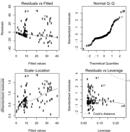
The output includes the row number of the minimum and maximum residual. Graphical tools are the best way to examine residuals. Figure 4.3 displays the default diagnostic plots (4.4) from the model.

> oldpar = par(mfrow=c(2, 2), mar=c(4, 4, 2, 2)+.1) > plot(lm1)

> par(oldpar)

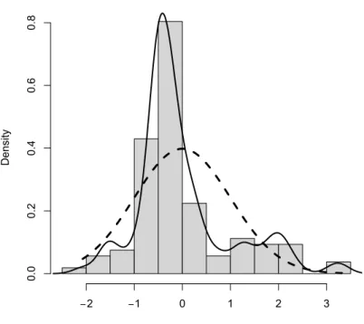
Figure 4.4 displays the empirical density of the standardized residuals, along with an overlaid normal density. The assumption that the residuals are ap-proximately Gaussian does not appear to be tenable.

> library(MASS)

> std.res = rstandard(lm1)

> hist(std.res, breaks=seq(-2.5, 3.5, by=.5), main="",

+ xlab="standardized residuals", col="gray80", freq=FALSE) > lines(density(std.res), lwd=2)

> xvals = seq(from=min(std.res), to=max(std.res), length=100) > lines(xvals, dnorm(xvals, mean(std.res), sd(std.res)), lty=2, + lwd=3)

(20)

0 10 20 30 40 �40 �20 0 20 40 60 Fitted values Residuals Residuals vs Fitted 4 84 77 �2 �1 0 1 2 �2 �1 0 1 2 3 Theoretical Quantiles Standardi zed residuals Normal Q−Q 4 84 77 0 10 20 30 40 0.0 0.5 1.0 1.5 Fitted values S ta nd ar di ze d re si du al s Scale−Location 4 84 77 0.00 0.10 0.20 �2 �1 0 1 2 3 4 Leverage Standardi zed residuals Cook's distance 0.5 Residuals vs Leverage 4 57 60

Figure 4.3: Default diagnostics.

The residual plots indicate some potentially important departures from model assumptions, and further exploration should be undertaken.

4.7.5

Fitting regression model separately for each value

of another variable

One common task is to perform identical analyses in several groups. Here, as an example, we consider separate linear regressions for each substance abuse group.

A matrix of the correct size is created, then aforloop is run for each unique value of the grouping variable.

(21)

4.7. HELP EXAMPLES 113 standardized residuals Density −2 −1 0 1 2 3 0.0 0.2 0.4 0.6 0.8

Figure 4.4: Empirical density of residuals, with superimposed normal density.

> uniquevals = unique(substance) > numunique = length(uniquevals) > formula = as.formula(i1 ~ age) > p = length(coef(lm(formula)))

> res = matrix(rep(0, numunique*p), p, numunique) > for (i in 1:length(uniquevals)) {

+ res[,i] = coef(lm(formula, subset=substance==uniquevals[i])) + }

> rownames(res) = c("intercept","slope") > colnames(res) = uniquevals

> res

heroin cocaine alcohol intercept -7.770 5.257 57.11 slope 0.393 0.116 -0.72

(22)

4.7.6

Two-way ANOVA

Is there a statistically significant association between gender and substance abuse group with depressive symptoms? The function interaction.plot()

can be used to graphically assess this question. Figure 4.5 displays an interac-tion plot for CESD as a funcinterac-tion of substance group and gender.

> attach(ds)

> sub = as.factor(substance)

> gender = as.factor(ifelse(female, "F", "M"))

> interaction.plot(sub, gender, cesd, xlab="substance", las=1, + lwd=2) 28 30 32 34 36 38 40 substance mean of cesd

alcohol cocaine heroin

gender F M

Figure 4.5: Interaction plot of CESD as a function of substance group and gender.

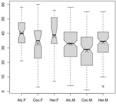
There are indications of large effects of gender and substance group, but little suggestion of interaction between the two. The same conclusion is reached in Figure 4.6, which displays boxplots by substance group and gender.

(23)

4.7. HELP EXAMPLES 115 > subs = character(length(substance)) > subs[substance=="alcohol"] = "Alc" > subs[substance=="cocaine"] = "Coc" > subs[substance=="heroin"] = "Her" > gen = character(length(female))

> boxout = boxplot(cesd ~ subs + gender, notch=TRUE, + varwidth=TRUE, col="gray80")

> boxmeans = tapply(cesd, list(subs, gender), mean) > points(seq(boxout$n), boxmeans, pch=4, cex=2)

Alc.F Coc.F Her.F Alc.M Coc.M Her.M

0 10 20 30 40 50 60 o

Figure 4.6: Boxplot of CESD as a function of substance group and gender. The width of each box is proportional to the size of the sample, with the notches denoting confidence intervals for the medians, and X’s marking the observed means.

Next, we proceed to formally test whether there is a significant interaction through a two-way analysis of variance (4.1.8). We fit models with and without an interaction, and then compare the results. We also construct the likelihood ratio test manually.

(24)

> aov1 = aov(cesd ~ sub * gender, data=ds) > aov2 = aov(cesd ~ sub + gender, data=ds) > resid = residuals(aov2)

> anova(aov2, aov1)

Analysis of Variance Table

Model 1: cesd ~ sub + gender Model 2: cesd ~ sub * gender

Res.Df RSS Df Sum of Sq F Pr(>F) 1 449 65515 2 447 65369 2 146 0.5 0.61 > options(digits=6) > logLik(aov1) 'log Lik.' -1768.92 (df=7) > logLik(aov2) 'log Lik.' -1769.42 (df=5)

> lldiff = logLik(aov1)[1] - logLik(aov2)[1] > lldiff

[1] 0.505055

> 1 - pchisq(2*lldiff, 2)

[1] 0.603472

> options(digits=3)

There is little evidence (p=0.61) of an interaction, so this term can be dropped. The model was previously fit to test the interaction, and can be displayed.

(25)

4.7. HELP EXAMPLES 117

> aov2

Call:

aov(formula = cesd ~ sub + gender, data = ds)

Terms:

sub gender Residuals Sum of Squares 2704 2569 65515 Deg. of Freedom 2 1 449

Residual standard error: 12.1 Estimated effects may be unbalanced

> summary(aov2)

Df Sum Sq Mean Sq F value Pr(>F) sub 2 2704 1352 9.27 0.00011 gender 1 2569 2569 17.61 3.3e-05 Residuals 449 65515 146

The default design matrix (lowest value is reference group, see 4.1.3) can be changed and the model refit. In this example, we specify the coding where the highest value is denoted as the reference group (which could allow matching results from a similar model fit in SAS).

> contrasts(sub) = contr.SAS(3)

> aov3 = lm(cesd ~ sub + gender, data=ds) > summary(aov3)

Call:

lm(formula = cesd ~ sub + gender, data = ds)

Residuals:

Min 1Q Median 3Q Max -32.13 -8.85 1.09 8.48 27.09

Coefficients:

Estimate Std. Error t value Pr(>|t|) (Intercept) 39.131 1.486 26.34 < 2e-16 sub1 -0.281 1.416 -0.20 0.84247 sub2 -5.606 1.462 -3.83 0.00014 genderM -5.619 1.339 -4.20 3.3e-05

Residual standard error: 12.1 on 449 degrees of freedom Multiple R-squared: 0.0745, Adjusted R-squared: 0.0683 F-statistic: 12 on 3 and 449 DF, p-value: 1.35e-07

(26)

The AIC criteria (4.2.3) can also be used to compare models: this also suggests that the model without the interaction is most appropriate.

> AIC(aov1)

[1] 3552

> AIC(aov2)

[1] 3549

4.7.7

Multiple comparisons

We can also carry out multiple comparison (4.3.4) procedures to test each of the pairwise differences between substance abuse groups. We use theTukeyHSD()

function here.

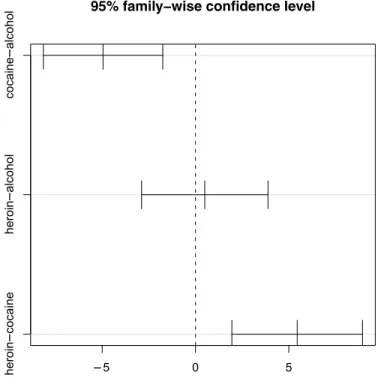
> mult = TukeyHSD(aov(cesd ~ sub, data=ds), "sub") > mult

Tukey multiple comparisons of means 95% family-wise confidence level

Fit: aov(formula = cesd ~ sub, data = ds)

$sub

diff lwr upr p adj cocaine-alcohol -4.952 -8.15 -1.75 0.001 heroin-alcohol 0.498 -2.89 3.89 0.936 heroin-cocaine 5.450 1.95 8.95 0.001

The alcohol group and heroin group both have significantly higher CESD scores than the cocaine group, but the alcohol and heroin groups do not significantly differ from each other (95% CI ranges from−2.8 to 3.8). Figure 4.7 provides a graphical display of the pairwise comparisons.

> plot(mult)

4.7.8

Contrasts

We can also fit contrasts (4.3.3) to test hypotheses involving multiple parame-ters. In this case, we can compare the CESD scores for the alcohol and heroin groups to the cocaine group.

(27)

4.7. HELP EXAMPLES 119 −5 0 5 heroin − cocaine heroin − alcohol cocaine − alcohol

95% family−wise confidence level

Differences in mean levels of sub

Figure 4.7: Pairwise comparisons.

> library(gmodels)

> fit.contrast(aov2, "sub", c(1,-2,1), conf.int=0.95 )

Estimate Std. Error t value Pr(>|t|) lower CI sub c=( 1 -2 1 ) 10.9 2.42 4.52 8.04e-06 6.17

upper CI sub c=( 1 -2 1 ) 15.7

As expected from the interaction plot (Figure 4.5), there is a statistically sig-nificant difference in this one degree of freedom comparison (p<0.0001).

(28)