Improving WPM2 for (Weighted) Partial
MaxSAT
⋆Carlos Ans´otegui1, Maria Luisa Bonet2, Joel Gab`as1, and Jordi Levy3 1 DIEI, Univ. de Lleida
[email protected] [email protected] 2 LSI, UPC [email protected] 3 IIIA-CSIC [email protected]
Abstract. Weighted Partial MaxSAT (WPMS) is an optimization variant of the Satisfiability (SAT) problem. Several combinatorial optimization problems can be translated into WPMS. In this paper we extend the state-of-the-art WPM2 algorithm by adding several improvements, and implement it on top of an SMT solver. In particular, we show that by focusing search on solving to optimality subformulas of the original WPMS instance we increase the efficiency of WPM2. From the experimental evaluation we conducted on the PMS and WPMS instances at the 2012 MaxSAT Evaluation, we can conclude that the new approach is both the best performing for industrial instances, and for the union of industrial and crafted instances.
1
Introduction
In the last decade Satisfiability (SAT) solvers have progressed dramatically in performance due to new algorithms, such as, conflict directed clause learning [36], and better implementation techniques. Thanks to these advances, nowadays the best SAT solvers can tackle hard decision problems. Our aim is to push this technology forward to deal with optimization problems.
The Maximum Satisfiability (MaxSAT) problem is the optimization version of SAT. The idea behind this formalism is that sometimes not all constraints of a problem can be satisfied, and we try to satisfy the maximum number of them. The MaxSAT problem can be further generalized to the Weighted Partial MaxSAT (WPMS) problem.
In the MaxSAT community, we find two main classes of algorithms: branch and bound [17, 22, 24, 26, 27] and SAT-based [2, 14, 19–21, 31–33]. The latter clearly dominate on industrial and some crafted instances, as we can see in the results of the last 2012 MaxSAT Evaluation. SAT-based MaxSAT algorithms
⋆
This research has been partially founded by the CICYT research projects TASSAT (TIN2010-20967-C04-01/03/04) and ARINF (TIN2009-14704-C03-01).
basically reformulate a MaxSAT instance into a sequence of SAT instances. By solving these SAT instances the MaxSAT problem can be solved [6].
In this paper we revisit the SAT-based MaxSAT algorithm WPM2 [5] which belongs to a family of algorithms that exploit the information from the unsatisfiable cores the underlying SAT solver provides. This algorithm is the natural extension to the weighted case of the Partial MaxSAT algorithm PM2 [4, 3]. In our experimental investigation the original WPM2 algorithm solves 796 out of 1474 from the whole benchmark of PMS and WPMS industrial and crafted instances at the 2012 MaxSAT Evaluation. We have extended WPM2 with several complementary improvements. First of all, we apply the stratification approach described in [2], what results in solving 74 additional instances. Secondly, we introduce a new criteria to decide when soft clauses can be hardened, that provides 66 additional solved instances. The hardening of soft clauses in MaxSAT SAT-based solvers has been previously studied in [2, 33]. Finally, our most effective contribution is to introduce a new strategy that focuses search on solving to optimality subformulas of the original MaxSAT instance. Actually, the new WPM2 algorithm is parametric on the approach we use to optimize these subformulas. This allows to combine the strength of exploiting the information extracted from unsatisfiable cores and other optimization approaches. By solving these smaller optimization problems we get the most significant boost in our new WPM2 algorithm. In particular, we experiment with three approaches: (i) refine the lower bound on these subformulas with the subsetsum function [13, 5], (ii) refine the upper bound with the strategy applied in minisat+ [15], SAT4J [10], qmaxsat [21] or ShinMaxSat [20], and (iii) a binary search scheme where the lower bound and upper bound are refined as in the previous approaches. The best performing approach in our experimental analysis is the second one and it allows to solve up to 238 additional instances. As a summary, the overall speed-up we achieved on the original WPM2 solver is about 378 additional solved instances, a 47% more. As we mentioned, SAT-based MaxSAT algorithms reformulate a MaxSAT instances into a sequence of SAT instances. Obviously, it is important to use an efficient SAT solver. Also, most SAT-based MaxSAT algorithms require the addition of Pseudo-Boolean (PB) linear constraints as a result of the reformulation process. These PB constraints are used to bound the cost of the optimal assignment. Currently, in most state-of-the-art SAT-based MaxSAT solvers, PB constraints are translated into SAT. However, there is no known SAT encoding which can guarantee the original propagation power of the constraint, i.e, what we call arc-consistency, while keeping the translation low in size. The best approach so far, has a cubic complexity [8]. This can be a bottleneck for WPM2 [5] and also for other algorithms such as, BINCD [19] or SAT4J [10].
In order to treat PB constraints with specialized inference mechanisms and a moderate cost in size, while preserving the strength of SAT techniques for the rest of the formula, we use the Satisfiability Modulo Theories (SMT) technology [35]. Related work in this sense can be found in [34]. Also, in [1] a Weighted Constraint
Satisfaction Problems (WCSP) solver implementing the original WPM1 [4] algorithm is presented.
An SMT instance is a generalization of a Boolean formula in which some propositional variables have been replaced by predicates with predefined interpretations from background theories such as, e.g., linear integer arithmetic. Most modern SMT solvers integrate a SAT solver with decision procedures (theory solvers) for sets of literals belonging to each theory. This way, we can hopefully get the best of both worlds: in particular, the efficiency of the SAT solver for the Boolean reasoning and the efficiency of special-purpose algorithms for the theory reasoning.
Another reasonable choice would be to use a PB solver, which can be seen as a particular case of an SMT solver specialized on the theory of PB constraints [28, 29]. However, if we also want to solve problems modeled with richer formalisms like WCSP, the SMT approach seems a better choice since we can take advantage of a wide range of theories [1].
In this work, we implemented both the last version of the WPM1 algorithm [2] and the revisited version of the WPM2 algorithm on top the of the SMT solver Yices. Then, we performed an extensive experimental evaluation comparing them with the best two solvers for PMS and WPMS categories at the 2012 MaxSAT Evaluation and with three additional solvers that did not take part but have been reported to exhibit good performance:bincd2, which is the new version of the BINCD algorithm [19] described in [33], with the best configuration reported by authors,maxhsfrom [14], which consists in an hybrid SAT and Integer Linear Programming (ILP) approach, andilp which performs a translation of WPMS into ILP solved with IBM-CPLEX studio124 [7].
We observe that the implementation on SMT of our new WPM2 algorithm with the second approach for optimizing the subformulas is the best performing solver for both PMS and WPMS industrial instances. We also observe that it is the best performing for the union of PMS and WPMS industrial and crafted instances, what shows this is a robust approach. These results make us conjecture that by improving the interaction of our new WPM2 algorithm with diverse optimization techniques applied on the subformulas we can get additional speed-ups.
This paper proceeds as follows. Section 2 presents some preliminary concepts. Section 3 describes WPM2 [5] and the new improvements. Section 4 describes the SMT problem and discuss some implementation details of the SMT-based MaxSAT algorithms. Section 5 presents the experimental evaluation. Finally, Section 6 shows the conclusions and the future work.
2
Preliminaries
A literal is either a Boolean variable x or its negation x. A clause C is a disjunction of literals. A weighted clause is a pair (C, w), where C is a clause and w is a natural number or infinity, indicating the penalty for falsifying the
clauseC. AWeighted Partial MaxSAT formulais a multiset of weighted clauses
ϕ={(C1, w1), . . . ,(Cm, wm),(Cm+1,∞), . . . ,(Cm+m′,∞)}
where the first m clauses are soft and the last m′ clauses are hard. The set of
variables occurring in a formulaϕis noted as var(ϕ).
A(total) truth assignment for a formula ϕis a function I: var(ϕ)→ {0,1}, that can be extended to literals, clauses and SAT formulas. For MaxSAT formulas is defined asI({(C1, w1), . . . ,(Cm, wm)}) =Pmi=1wi(1−I(Ci)). The
optimal cost of a formula is cost(ϕ) = min{I(ϕ)|I : var(ϕ) → {0,1}}and an
optimal assignment is an assignmentI such thatI(ϕ) = cost(ϕ).
The Weighted Partial MaxSAT problem for a Weighted Partial MaxSAT formulaϕis the problem of finding anoptimal assignment.
3
WPM2 algorithm
The WPM2 algorithm [5] is described in Algorithm 1. The fragments in gray (lines 4, 10, 11, 13- 18 and 20) correspond to the new improvements we have incorporated.
In the WPM2 algorithm, we extend soft clauses Ci with a unique fresh
auxiliary blocking variable bi obtaining ϕw={Ci∨bi}i=1...m∪ {Cm+i}i=1...m′.
Notice that bi will be set to true by a SAT solver on ϕw if Ci is false. We
also work with a set AL of at-least PB constraints of the formP
i∈Awibi ≥k
on the variables bi, and a similar set AM of at-most constraints of the form
P
i∈Awibi≤k, that are modified at every iteration of the algorithm.
Intuitively, the WPM2 algorithm refines at every iteration the lower bound on
ϕtill it reaches the optimumcost(ϕ). TheAMconstraints are used to bound the cost of the falsified clauses. TheAL constraints are used to impose that subsets of soft clauses have a minimum cost and to compute the AM constraints, as we will see later. The algorithm ends when ϕw∪CN F(AL∪AM) becomes
satisfiable4, where CNF is the translation to SAT of the PB constraints.
Technically speaking, theALconstraints give lower bounds on cost(ϕ). The
AM constraints enforce that all solutions of the set of constraints AL∪AM
are the solutions of AL of minimal cost. This ensures that any solution of the formula sent to the solver,ϕw∪CNF(AL∪AM), if there is any, is an optimal
assignment of ϕ. Therefore, given a set of at-least constraints AL we compute a corresponding set of at-most constraints AM as follows. First, we need to introduce the notion of core and cover. A core is a set of indexes A such that
P
i∈Awibi ≥k ∈AL. Functioncore(
P
i∈Awibi ≥k) returns the core A and
functioncores(AL) returns{core(al)|al∈AL}. Covers are defined from cores as follows.
Definition 1. Given a set of coresL, we say that the set of indexesAis acover
ofL, if it is a minimal non-empty set such that, for every A′∈
L, ifA′∩ A6=∅, thenA′ ⊆
A. Given a set of coresL, we denote the set of covers ofL asSC(L).
4
TheALconstraints are redundant, i.e., not required to be sent to the SAT solver for the soundness of the algorithm but help to speed up the search.
Algorithm 1: Revisited WPM2 algorithm.
Input:ϕ={(C1, w1), . . . ,(Cm, wm),(Cm+1,∞), . . . ,(Cm+m′,∞)} 1: if sat({Ci∈ϕ|wi=∞}) = (U N SAT, , )then return(∞,∅)
2: ϕw:={C1∨b1, . . . , Cm∨bm, Cm+1, . . . , Cm+m′} ⊲Extend all soft clauses 3: AL:={w1b1≥0, . . . , wmbm≥0} ⊲Set of at-least constraints
4: wmax:=∞
5: whiletruedo
6: AM:=∅ ⊲Set of at-most constraints
7: foreach(P
i∈Awibi≥k)∈ALdo 8: if A∈SC(cores(AL))then 9: AM:=AM∪ {P
i∈Awibi≤k}
10: (st, ϕc,I) :=sat(ϕw\{Ci∨bi |(Ci, wi)∈ϕ∧wi< wmax}∪CNF(AL∪AM))
11: if st=satand wmax= 0then return(I(ϕ),I)
12: else
13: if st=satthen
14: W:=P{wi|(Ci, wi)∈ϕ∧wi< wmax}
15: ϕh:=harden(ϕ, AM, W)
16: wmax:=decrease(wmax, ϕ)
17: else 18: A:={i|(Ci∨bi)∈(ϕc\ϕh)} ⊲New core 19: A:=SA′ ∈cores(AL) A′ ∩A6=∅ A′ ⊲New cover 20: k:=newbound(AL∪ϕw, A) 21: AL:={al∈AL|core(al)6=A} ∪ {Pi ∈Awibi≥k}
Given a setAL, the setAM is the set of at-most constrainsP
i∈Awibi≤k
such that A ∈ SC(cores(AL)) andk is the solution of minimizingP
i∈Awibi
subject toAL andbi∈ {0,1}.
The algorithm starts with AL = {w1b1 ≥ 0, . . . , wmbm ≥ 0} and the
correspondingAM :={w1b1≤0, . . . , wmbm≤0} that ensures that the unique
solution of AL∪AM is b1 = · · · = bm = 0 with cost 0 5. At every iteration,
the algorithm calls a SAT solver with ϕw∪CNF(AL∪AM). If it returnssat,
then the interpretationI is a MaxSAT solution ofϕand we return the optimal costI(ϕ). If it returns unsat, then we use the information of the unsatisfiable core ϕc obtained by the SAT solver to enlarge the set AL, excluding more
interpretations on the bi’s that are not partial solutions of ϕw. Before calling
again the SAT solver, we update AM conveniently, to ensure that solutions to the new constraintsAL∪AMare still minimal solutions of the newALconstraint set. Notice that in every iteration the set of solutions of{b1, . . . , bm}defined by
ALis decreased, whereas the set of solutions ofAM is increased.
5
In the implementation, we do not add a blocking variable to a soft clause till it appears into a core.
One key point in WPM2 is to compute thenewbound(AL, A) (line 20) which corresponds to the following optimization problem:
minimizeX i∈A wi·bi subject to { X i∈A wi·bi≥k} ∪AL (1) wherek= 1 +P {k′ | P i∈A′wibi≤k′∈AM∧A′⊆A}.
Notice that by removing the AL constraints in (1), we get the subsetsum problem [13]. In the original WPM2 algorithm [5], the subsetsum problem is progressively solved until we get a solution that also satisfies theALconstraints. This satisfiability check in the original WPM2 is performed with a SAT solver.
In what follows, we present how we have modified the original WPM2 algorithm (fragments in gray in Algorithm 1) by incorporating several improvements: the application of a stratified approach, the hardening of soft clauses and the optimization of the subformulas defined by the covers.
3.1 Stratified Approach
As in [4] for WPM1, we apply a stratified approach. The stratified approach (lines 4, 10, 11 and 16) consists in sending to the SAT solver only those soft clauses with weight wi ≥wmax. Then, when the SAT solver returns sat, if there are still unsent clauses, we decrease wmax to include additional clauses
to the formula. From [4], we also apply the diversity heuristic (line 16) which supplies us with an efficient method to calculate how we have to reduce the value ofwmaxin the stratified approach, so that, when there is a big variety of
distinct weights,wmaxdecreases faster, and, when there is a low diversity,wmax
is decreased to the following value of wi. Similar approach with an alternative
heuristic for grouping clauses can be found in [32].
3.2 Clause Hardening
The hardening of soft clauses in MaxSAT SAT-based solvers has been previously studied in [11, 25, 23, 18, 30, 2, 33]. Inspired by these works we study a hardening scheme for WPM2. While clause hardening was reported to have no positive effect in WPM1 [2], we will see that it boosts efficiency in WPM2.
The clause hardening (lines 14, 15 and 18) consists in considering hard those soft clauses whose satisfiability we know does not need to be reconsidered. We need some lemma ensuring that falsifying those soft clauses would lead us to suboptimal solutions. In the case of WPM1, all soft clauses satisfyingwi> W,
whereW =P{w
i|(Ci, wi)∈ϕ∧wi< wmax}is the sum of weights of clauses not
sent to the SAT solver, can be hardened. The correctness of this transformation is ensured by the following lemma:
Lemma 1 (Lemma 24 in [6]).
Let ϕ1 = {(C1, w1), . . . ,(Cm, wm),(Cm+1,∞), . . . ,(Cm+m′,∞)} be a
MaxSAT formula with cost zero, letϕ2={(C′ 1, w′ 1), . . . ,(C ′ r, w ′ r)}be a MaxSAT
formula without hard clauses andW =Pr j=1w ′ j. Let harden(w) = w if w≤W ∞if w > W andϕ′
1={(Ci,harden(wi))|(Ci, wi)∈ϕ1}. Then,cost(ϕ1∪ϕ2) = cost(ϕ′1∪ϕ2),
and any optimal assignment forϕ′
1∪ϕ2 is an optimal assignment ofϕ1∪ϕ2.
However, this lemma is not useful in the case of WPM2 because we do not proceed by transforming the formula, like in WPM1. Therefore, we generalize this lemma. For this, we need to introduce the notion of optimal of a formula.
Definition 2. Given a MaxSAT formula ϕ = {(C1, w1), . . . ,(Cm, wm),
(Cm+1,∞), . . . ,(Cm+m′,∞)}, we say thatk is a (possible) optimal ofϕif there
exists a subsetA⊆ {1, . . . , m} such thatP
i∈Awi=k.
Notice that, for any interpretationIof the variables ofϕ, we have thatI(ϕ) is an optimal ofϕ. However, ifkis an optimal, there does not exist necessarily an interpretationIsatisfyingI(ϕ) =k. Notice also that, givenϕandk, finding thenext optimal, i.e. finding the smallestk′
> ksuch thatk′ is an optimal of ϕ
is equivalent to the subset sum problem.
Lemma 2. Let ϕ1∪ϕ2 be a MaxSAT formula andk1 andk2 values such that:
cost(ϕ1∪ϕ2) =k1+k2and any assignmentIsatisfiesI(ϕ1)≥k1andI(ϕ2)≥k2. Let k′ be the smallest possible optimal of
ϕ2 such thatk′
> k2. Letϕ3 be a set of soft clauses with W =P
{wi|(Ci, wi)∈ϕ3}.
Then, ifW < k′−k2, then any optimal assignmentI′ofϕ1∪ϕ2∪ϕ3assigns I′(ϕ2) =k2
Proof. LetI′ be any optimal assignment of
ϕ1∪ϕ2∪ϕ3. On the one hand, as for any other assignment, we haveI′(
ϕ2)≥k2.
On the other hand, any of the optimal assignments I of ϕ1∪ϕ2 can be extended (does not matter how) to the variables of var(ϕ3)\var(ϕ1∪ϕ2), such that
I(ϕ1∪ϕ2∪ϕ3) =I(ϕ1) +I(ϕ2) +I(ϕ3)≤k1+k2+W < k1+k′
(2) Now, assume that I′(
ϕ2)6=k2, thenI′(
ϕ2)≥k′. As any other assignment, I′(
ϕ1) ≥ k1. Hence, I′(
ϕ1∪ϕ2 ∪ϕ3) ≥ k1+k′
> I(ϕ1∪ϕ2∪ϕ3), but this contradicts the optimality ofI′. Therefore,
I′(
ϕ2) =k2.
⊓ ⊔
In order to apply this lemma we have to consider partitions of the formula
ϕ1∪ϕ2ensuring cost(ϕ1∪ϕ2) =k1+k2andI(ϕ1)≥k1andI(ϕ2)≥k2, for any assignmentI. This can be easily ensured, in the case of WPM2, if bothϕ1 and
ϕ2are unions of covers. Then, we only have to check if the next possible optimal
k′ of
ϕ2 exceeds the previous one k2 more than the sum W of the weights of the clauses not sent to the SAT solver. In such a case, we can consider all soft
clauses ofϕ2and their correspondingAM constraint withk2as hard clauses. In other words, we do not need to recompute the partial optimal k2 ofϕ2.
Finally, in line 15 of Algorithm 1, function harden(ϕ, AM, W) returns the set of soft clauses ϕh that needs to be considered hard based on the previous
analysis according to: the current set of covers AM, the next optimals of these covers and the sum of the weights W of soft clauses beyond the currentwmax,
i.e., not yet sent to the SAT solver.
3.3 Cover Optimization
As we have mentioned earlier, one key point in WPM2 is how to compute the
newbound(AL, A) (line 20). Actually, we can solve to optimality the subformulas defined by the union of the soft clauses related to the cover A and the hard clauses.
Definition 3. Given a MaxSAT formula ϕ = {(C1, w1), . . . ,(Cm, wm),
(Cm+1,∞), . . . ,(Cm+m′,∞)} and a set of indexesA, we define the subformula, ϕ[A], as follows: ϕ[A] ={(Ci, wi)∈ϕ|i∈A∨wi =∞)}
Solving to optimalityϕ[A] give us the optimal value k=cost(ϕ[A]) for the
AM constraint related to cover A. In order to do this, while taking advantage of theALconstraints generated so far, we only have to extend the minimization problem corresponding to the newbound (1) function, by adding ϕw to the
constraints, i.e,newbound(AL∪ϕw, A)6. Notice thatnewbound(AL∪ϕw, A)≥
newbound(AL, A).
In order to optimize ϕ[A], we can use any exact approach related to MaxSAT, such as, MaxSAT branch and bound algorithms, MaxSAT SAT-based algorithms, saturation under the MaxSAT resolution rule, or we can use other solving techniques such as PB solvers or ILP techniques, etc. Our new WPM2 algorithm is parametric on any suitable optimization solving approach. In this work, we present three approaches.
The first and natural approach consists in iteratively refining (increasing) the lower bound on the optimal kforϕ[A] by applying the subsetsum function as in the original WPM2. The procedure stops when we satisfy the constraints
AL∪ϕw. Notice that since we have includedϕw into the set of constraints, the
solution we will eventually get has to be optimal forϕ[A].
The second approach consists in iteratively refining (decreasing) the upper bound following the strategy applied in minisat+ [15], SAT4J [10], qmaxsat [21] or ShinMaxSat [20]. The upper boundubis initially set to the sum of the weights
wi of the soft clauses in ϕ[A]. Then, we iteratively test whetherk =ub−1 is
feasible or not. Whenever we get a satisfying assignment, we update ubto the sum of the weightswi of those soft clauses wherebi evaluates to true under the
satisfying assignment. If we get an unsatisfiable answer, the previous ubis the optimal value forϕ[A].
6 We can actually exclude from
The third approach applies a binary search scheme [19, 12, 16]. We additionally refine the lower bound as in our first approach and the upper bound as in the second approach.
The worst case complexity, in terms of the number of calls to the SAT solver, of the new WPM2 algorithm is the number of times that the newbound function is called (bounded by the number of clauses) multiplied by the number of SAT calls needed in each call to the newbound function. This latter number is logarithmic on the sum of the weights of the clauses of the core if we use a binary search, hence essentially the number of clauses. Therefore, the worst case complexity, when using a binary search to solve to optimality the subformulas, is quadratic on the number of soft clauses.
In order to see that the number of calls to the newbound function is bounded by the number of clauses we just need to recall that WPM2 merges the covers. Consider a binary tree where the soft clauses are the leaves, and the internal nodes represent the merges (calls to the newbound function). A binary tree of n leaves has n-1 internal nodes.
Solving to optimality all the covers can be very costly since these are NP-hard problems. Depending on the unsatisfiable cores we get in the general loop of the WPM2 algorithm some covers have to be merged. Therefore, we may argue that part of the work we did in order to optimize these covers can be useless 7. For
example, a reasonable strategy is to optimize the current cover only if it was not the result of merging other covers, i.e., when the last unsatisfiable core is contained into a cover. In the experimental evaluation, we will see that although the number of solved instances does not vary too much, the mean time for solving some families can be decreased.
4
Engineering Efficient SMT-based MaxSAT Solvers
We have implemented both the last version of the WPM1 algorithm [2] and the revisited version of the WPM2 algorithm on top the of the SMT solver Yices.
As we have said, an SMT instance is a generalization of SAT where some propositional variables are replaced by predicates with predefined interpretations from background theories. Among the theories considered in the SMT library [9] we are interested in QF LIA (Quantifier-FreeLinear Integer Arithmetic). With the QF LIA theory we can model the PB constraints that SAT-based MaxSAT algorithms generate during their execution. Therefore, for the SMT-based MaxSAT algorithm, we just need to replace the conversion to CNF (line 10 in Algorithm 1) by the proper linear integer arithmetic predicates.
As suggested in [16, 31], we can preserve some learned lemmas from previous iterations that may help to reduce the search space. In order to do that, we execute the SMT solver in incremental mode. Within this mode, we can call the solve routine and add new clauses (assertions) on demand, while preserving learned lemmas. However, notice that our algorithms delete parts of the formula
7 The related
between iterations. For example, in lines 7 to 9 of Algorithm 1 we recompute the set AM, possibly erasing some of the at-most constraints. Therefore, we have to take care also of any learned lemma depending on them.
The SMT solver Yices gives the option of marking assertions asretractable. If the SMT solver does not support the deletion of assertions but supports the usage of assumptions, we can replace every retractable assertionC, witha→C, where
a is an assumption. Before each call, we activate the assumptions of assertions that have not been retracted by the algorithm. Notice that assertions that do have been retracted will have a pure literal (a) such thatahas not been activated. Therefore, the solver can safely set to falseadeactivating the clause. Moreover, any learned lemma on those assertions will also includea. For example, Z3 and Mathsat SMT solvers do not allow to delete clauses, but they allow the use of assumptions.
5
Experimental Results
In this section we present an intensive experimental investigation on the PMS and WPMS industrial and crafted instances from the 2012 MaxSAT Evaluation. We provide results for our new WPM2 SMT-based MaxSAT solver, for a WPM1 [2] SMT-based MaxSAT solver, the best two solvers for each category of the 2012 MaxSAT Evaluation, and three solvers which did not participate but the authors have reported to exhibit good performance. We run our experiments on a cluster featured with 2.27 GHz processors, memory limit of 3.9 GB and a timeout of 7200 seconds per instance.
The experimental results are presented in Tables 1 and 2 following the same classification criteria as in the 2012 MaxSAT Evaluation. For each solver and family of instances, we present the number of solved instances in parenthesis and the mean solving time. Solvers are ordered from left to right according to the total number of solved instances. The results for the best performing solver in each family are presented in bold. The number of instances of every family is specified in the column under the sign ’#’. Since different families may have different number of instances, we also include for each solver the mean ratio of solved instances.
Our new WPM2 algorithm is implemented on top of the Yices SMT solver (version 1.0.29). The different versions of WPM2 and corresponding implementations are named wpm2 where subindexes can be s that stands for
stratified approach with diversity heuristic and h for hardening. Regarding to
how we perform the cover optimization, l stands for lower bound refinement
based on subsetsum, u for upper bound refinement based on satisfying truth
assignment, and b for binary search. Finally, a stands for optimizing all the
covers andc for optimizing only covers that contain the last unsatisfiable core.
Table 1 shows our first experiment, where we evaluate the impact of each variation on the originalwpm2. By using a stratified approach with the diversity heuristic (wpm2s) we solve some additional instances in all categories having
Instance set # wpm2 wpm2s wpm2sh wpm2shlc wpm2shla wpm2shbc wpm2shba wpm2shuc wpm2shua PMS-Industrial aes 7 0.00(0) 0.00(0) 0.00(0) 0.00(0) 0.00(0) 0.00(0) 10.34(1) 1836.54(1) 514.14(1) bcp-fir 59 83.29(57) 23.44(57) 23.44(57) 40.87(57) 104.75(57) 113.13(57) 146.03(57) 60.91(58) 57.36(58) bcp-hipp-yRa1 simp 17 504.81(13) 155.95(12) 155.95(12) 95.16(12) 239.17(13) 151.30(13) 813.36(16) 107.24(16) 160.55(16) bcp-hipp-yRa1 su 38 380.47(19) 164.70(16) 164.70(16) 181.49(18) 667.59(19) 226.66(25) 585.82(28) 555.92(33) 315.87(34) bcp-msp 64 821.88(25) 756.59(26) 756.59(26) 283.50(28) 606.35(28) 283.78(31) 464.47(30) 711.08(36) 912.70(34) bcp-mtg 40 1363.97(18) 852.58(23) 852.58(23) 1320.80(28) 786.09(34) 1296.44(32) 940.62(37) 997.38(35) 578.75(39) bcp-syn 74 60.29(41) 302.54(41) 302.54(41) 296.12(41) 83.15(39) 242.78(42) 69.23(42) 103.21(43) 78.22(42) circuit-trace-compaction 4 285.74(3) 835.72(4) 835.72(4) 230.85(3) 134.79(4) 145.72(4) 151.41(4) 118.24(4) 129.10(4) haplotype-assembly 6 2.87(5) 7.17(5) 7.17(5) 9.80(5) 42.86(5) 15.53(5) 51.44(5) 18.28(4) 65.94(5) pbo-mqc nencdr 84 866.38(84) 821.16(84) 821.16(84) 142.43(84) 107.70(84) 130.90(84) 127.99(84) 245.77(84) 257.06(84) pbo-mqc nlogencdr 84 362.20(84) 353.14(84) 353.14(84) 24.48(84) 17.19(84) 58.42(84) 65.79(84) 124.43(84) 140.44(84) pbo-routing 15 0.46(15) 2.14(15) 2.14(15) 3.89(15) 6.59(15) 4.88(15) 6.72(15) 5.42(15) 6.73(15) protein-ins 12 2626.34(10) 2162.13(9) 2162.13(9) 476.03(12) 552.46(12) 360.76(12) 284.63(12) 234.31(12) 333.85(12) Total 504 374 376 376 387 394 404 415 425 428 69.6% 70.9% 70.9% 72.5% 76.0% 77.5% 81.4% 81.7% 83.6% WPMS-Industrial haplotyping-pedigrees 100 16.01(22) 292.29(25) 242.08(90) 154.12(92) 142.59(92) 199.61(96) 86.67(95) 202.70(98) 176.02(98) timetabling 26 1017.27(8) 720.89(8) 651.84(8) 1008.59(9) 430.67(9) 1544.43(9) 931.17(8) 932.77(8) 1438.59(9) upgradeability-problem 100 19.19(100) 19.67(100) 15.27(100) 96.88(100) 375.70(100) 99.51(100) 365.70(100) 97.83(100) 371.96(100) Total 226 130 133 198 201 201 205 203 206 207 50.9% 51.9% 73.6% 75.5% 75.5% 76.9% 75.3% 76.3% 77.5% Total Industrial 730 504 509 574 588 595 609 618 631 635 66.1% 67.3% 71.4% 73.0% 75.9% 77.4% 80.2% 80.7% 82.5% PMS-Crafted frb 25 0.00(0) 0.00(0) 0.00(0) 0.00(0) 0.00(0) 0.00(0) 0.00(0) 0.00(0) 0.00(0) job-shop 3 68.31(3) 63.37(3) 63.37(3) 50.84(3) 53.11(3) 51.29(3) 49.87(3) 88.41(3) 58.75(3) maxclicque random 96 478.65(76) 471.97(76) 471.97(76) 435.07(77) 533.97(78) 423.89(83) 392.04(82) 565.44(87) 512.17(89) maxclicque structured 62 779.71(21) 592.07(21) 592.07(21) 511.52(22) 783.37(24) 650.87(25) 838.38(26) 802.09(26) 876.90(27) maxone 3sat 80 16.42(80) 18.11(80) 18.11(80) 10.90(80) 9.39(80) 5.34(80) 5.29(80) 6.65(80) 6.47(80) maxone structured 60 156.20(58) 89.15(59) 89.15(59) 14.42(60) 32.46(60) 13.11(60) 46.68(60) 9.24(60) 50.43(60) min-enc kbtree 42 1607.47(4) 707.46(4) 707.46(4) 2057.16(5) 2086.38(5) 2254.64(6) 1777.41(5) 921.09(6) 1906.23(5) pseudo miplib 4 122.23(4) 93.95(4) 93.95(4) 109.21(4) 64.35(4) 27.35(4) 37.81(4) 54.30(4) 34.23(4) Total 372 246 247 247 251 254 261 260 266 268 64.9% 65.1% 65.1% 65.9% 66.5% 67.6% 67.4% 68.4% 68.5% WPMS-Crafted auc-paths 86 0.00(0) 376.67(1) 370.25(1) 706.38(33) 546.57(33) 1019.93(74) 948.64(75) 435.71(82) 271.16(82) auc-scheduling 84 0.00(0) 133.39(51) 136.89(51) 71.37(84) 69.59(84) 2.73(84) 1.66(84) 1.25(84) 1.07(84) min-enc-planning 56 491.39(25) 141.80(38) 138.29(38) 3.24(56) 2.47(56) 0.75(56) 0.77(56) 0.74(56) 0.80(56) min-enc-warehouses 18 11.36(1) 3.36(1) 3.43(1) 0.07(1) 0.08(1) 0.04(1) 0.05(1) 1227.86(2) 0.05(1) pseudo-miplib 12 2936.02(3) 1533.63(3) 1487.40(3) 13.72(3) 11.81(3) 471.93(4) 990.65(5) 299.53(4) 695.31(5) random-net 74 0.00(0) 0.00(0) 0.00(0) 1041.56(15) 1943.41(17) 1633.69(33) 1529.94(33) 3369.16(17) 3151.03(15) wcsp-spot5-dir 21 187.40(9) 310.45(10) 248.53(12) 420.10(14) 428.10(14) 495.17(14) 470.92(14) 8.27(14) 113.90(14) wcsp-spot5-log 21 1067.69(8) 469.38(10) 120.60(9) 100.07(13) 59.16(13) 133.75(14) 48.91(13) 23.84(14) 16.50(14) Total 372 46 114 115 219 221 280 281 273 271 19.5% 31.9% 32.5% 52.2% 52.6% 62.9% 63.4% 62.0% 62.0% Total Crafted 744 292 361 362 470 475 541 541 539 539 42.2% 48.5% 48.8% 59.1% 59.5% 65.2% 65.4% 65.2% 65.3% Total (W)PMS 1474 796 870 936 1058 1070 1150 1159 1170 1174 54.1% 57.9% 60.1% 66.1% 67.7% 71.3% 72.8% 72.9% 73.9% T a b le 1 . E xp er im en ta l re su lt s o f d iff er en t v er sio n s o f w p m 2 . 11
(a) Partial Industrial
Instance set # wpm2shua bincd2 qms0.21g2 pwbo2.1 shinms wpm1 ilp aes 7 514.14(1) 453.22(1) 3154.99(1) 0.00(0) 0.00(0) 3073.19(1) 1310.95(3) bcp-fir 59 57.36(58) 44.09(58) 108.17(56) 68.10(56) 13.54(22) 10.87(57) 62.86(59) bcp-hipp-yRa1 simp 17 160.55(16) 170.49(16) 358.14(17) 174.98(15) 40.66(16) 70.27(16) 666.94(6) bcp-hipp-yRa1 su 38 315.87(34) 244.97(32) 105.60(35) 97.91(25) 282.26(34) 244.23(28) 0.00(0) bcp-msp 64 912.79(34) 213.47(38) 451.50(30) 96.14(26) 281.37(22) 1053.47(7) 855.96(37) bcp-mtg 40 578.75(39) 1.15(40) 0.15(40) 0.57(40) 0.60(40) 8.54(40) 769.27(29) bcp-syn 74 78.22(42) 28.56(43) 283.64(35) 21.82(39) 86.98(33) 59.30(45) 18.95(71) circuit-trace-compaction 4 129.10(4) 109.31(4) 45.01(4) 200.11(2) 52.22(4) 118.43(4) 6921.80(1) haplotype-assembly 6 65.94(5) 728.30(5) 153.22(5) 9.09(5) 0.00(0) 2.63(5) 2124.72(5) pbo-mqc nencdr 84 257.06(84) 278.45(84) 58.78(84) 222.19(68) 145.71(84) 804.25(54) 1109.89(6) pbo-mqc nlogencdr 84 140.44(84) 78.58(84) 23.69(84) 71.86(82) 180.37(79) 403.38(55) 508.21(6) pbo-routing 15 6.73(15) 1.14(15) 3.61(15) 27.67(15) 4.80(15) 1.75(15) 19.68(15) protein-ins 12 333.85(12) 314.09(3) 128.58(12) 0.11(1) 206.51(4) 1812.03(3) 2.72(1) Total 504 428 423 418 374 353 330 239 Mean ratio 83.6% 78.2% 83.0% 66.3% 63.6% 68.3% 48.9%
(b) Weighted Partial Industrial
Instance set # wpm2shua wpm1 pwbo2.1 bincd2 maxhs ilp shinms haplotyping-pedigrees 100 176.02(98) 212.76(93) 123.00(87) 544.80(73) 1089.24(39) 1892.16(18) 1203.99(47) timetabling 26 1438.59(9) 1347.39(11) 671.45(7) 168.55(8) 1249.85(6) 0.00(0) 2261.00(5) upgradeability-problem 100 371.96((100) 4.57(100) 32.67(100) 76.40(100) 13.41(100) 19.26(100) 0.00(0) Total 226 207 204 194 181 145 118 52 Mean ratio 77.5% 78.4% 71.3% 67.9% 54.0% 39.3% 22.1% (c) Partial Crafted
Instance set # ilp akms ls qms0.21 shinms wpm2shua bincd2 pwbo2.1 wpm1 frb 25 1152.97(13) 159.47(5) 346.73(25) 43.52(23) 0.00(0) 0.00(0) 151.16(15) 0.00(0) job-shop 3 0.00(0) 0.00(0) 41.51(3) 36.44(3) 58.75(3) 100.43(3) 93.17(1) 835.23(3) maxclicque random 96 45.13(96) 1.09(96) 269.93(83) 339.30(76) 512.17(89) 85.29(71) 79.45(64) 652.31(59) maxclicque structured 62 326.51(38) 281.51(41) 800.18(30) 401.45(23) 876.90(27) 109.21(21) 37.07(19) 153.39(13) maxone 3sat 80 13.12(80) 0.47(80) 198.39(80) 694.52(78) 6.47(80) 8.28(80) 36.97(63) 97.24(80) maxone structured 60 337.60(59) 482.29(38) 6.35(60) 3.53(59) 50.43(60) 57.42(60) 7.71(60) 718.41(42) min-enc kbtree 42 162.89(42) 3199.18(34) 248.02(6) 513.97(5) 1906.23(5) 274.79(6) 306.58(2) 2469.35(6) pseudo miplib 4 34.12(4) 258.91(3) 1.84(4) 3.44(4) 34.23(4) 48.74(4) 93.19(4) 163.61(4) Total 372 332 297 291 271 268 245 228 207 Mean ratio 76.5% 63.2% 81.1% 77.0% 68.5% 65.3% 59.3% 58.3%
(d) Weighted Partial Crafted
Instance set # ilp wpm1 wpm2shua shinms akms ls pwbo2.1 maxhs bincd2 auc-paths 86 0.49(86) 108.14(63) 271.16(82) 317.62(84) 2.57(86) 110.67(19) 35.41(86) 1414.73(12) auc-scheduling 84 0.38(84) 1.56(84) 1.07(84) 5.81(84) 68.27(84) 7.65(81) 965.10(78) 141.77(81) min-enc-planning 56 296.52(56) 2.61(53) 0.80(56) 8.15(52) 141.21(40) 0.46(56) 459.18(31) 32.74(54) min-enc-warehouses 18 0.49(18) 78.89(17) 0.05(1) 0.43(1) 20.11(2) 3.78(14) 0.18(1) 2.10(1) pseudo-miplib 12 82.82(3) 157.33(4) 695.31(5) 127.99(5) 0.26(2) 3.97(3) 0.03(1) 1072.69(4) random-net 74 532.74(59) 4.03(70) 3151.03(15) 0.00(0) 4060.60(8) 42.15(35) 2770.76(10) 0.00(0) wcsp-spot5-dir 21 42.88(18) 37.70(13) 113.90(14) 743.63(21) 1555.46(6) 61.89(8) 101.11(6) 127.73(12) wcsp-spot5-log 21 322.93(8) 399.59(14) 16.50(14) 200.73(17) 108.70(5) 1.71(6) 357.32(6) 299.32(13) Total 372 332 318 271 264 233 222 219 177 Mean ratio 78.6% 77.4% 62.0% 64.8% 45.3% 54.4% 41.6% 45.6% T a b le 2 . E xp er im en ta l re su lt s o f b es t w p m 2 v er sio n co m p a re d w it h o th er so lv er s. 12
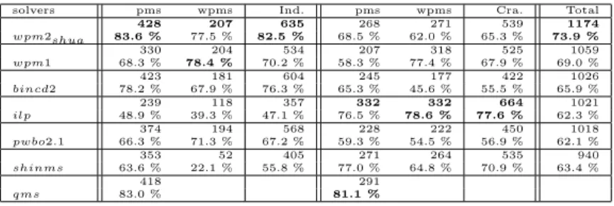
solvers pms wpms Ind. pms wpms Cra. Total 428 207 635 268 271 539 1174 wpm2shua 83.6 % 77.5 % 82.5 % 68.5 % 62.0 % 65.3 % 73.9 % 330 204 534 207 318 525 1059 wpm1 68.3 % 78.4 % 70.2 % 58.3 % 77.4 % 67.9 % 69.0 % 423 181 604 245 177 422 1026 bincd2 78.2 % 67.9 % 76.3 % 65.3 % 45.6 % 55.5 % 65.9 % 239 118 357 332 332 664 1021 ilp 48.9 % 39.3 % 47.1 % 76.5 % 78.6 % 77.6 % 62.3 % 374 194 568 228 222 450 1018 pwbo2.1 66.3 % 71.3 % 67.2 % 59.3 % 54.5 % 56.9 % 62.1 % 353 52 405 271 264 535 940 shinms 63.6 % 22.1 % 55.8 % 77.0 % 64.8 % 70.9 % 63.4 % 418 291 qms 83.0 % 81.1 %
Table 3.Summary of solved instances and mean ratio % for best solvers.
By adding hardening (wpm2sh) we solve 66 more instances, mainly in WPMS
industrial familyhaplotyping-pedigrees.
Regarding our three approaches for optimizing the covers, we can see that by optimizing with subsetsum (wpm2shla) we solve some additional instances in all
categories having the best improvement in WPMS industrial with 18 more and in WPMS crafted with 106 more. It is important to highlight that optimizing covers with subsetsum, instead of applying the subsetsum as in the original WPM2 algorithm, leads to a total improvement of 134 additional solved instances, with respect to wpm2sh.
Optimizing all covers by refining the upper bound (wpm2shua), we get an
additional boost with respect to wpm2shla. We can see that we solve some
additional instances in all categories. We get the best improvement for PMS industrial, solving 34 additional instances, and for WPMS crafted, 50 more. Notice that the overall increase with respect to wpm2sh is of 238 additional
solved instances.
Binary search (wpm2shba) improves 10 instances in WPMS crafted with
respect towpm2shua. But the global performance with respect towpm2sh, 223,
is not as good as only refining the upper bound (wpm2shua).
Optimizing only covers that contain the last unsatisfiable core solves almost the same instances as optimizing all covers but improves the average running time in the WPMS industrial familyupgradeability-problem by a factor of 4.
Table 2 shows the results of our second experiment where we compare the best variation and implementation of our new WPM2 algorithm (wpm2shua) with
several solvers. In particular, we compare with the best two solvers for the PMS and WPMS industrial and crafted instances of the 2012 MaxSAT Evaluation: PMS industrial (qms0.21g2, pwbo2.1), WPMS industrial (pwbo2.1 [31, 32],
wpm1 [2] 8
), PMS crafted (qms0.21 [21], akms ls [22] and WPMS crafted (wpm1,shinms[20]). We also compare with three additional MaxSAT solvers:
bincd2 , which is the new version of the BINCD algorithm [19] described in [33], with the best configuration reported by authors,maxhsfrom [14], which consists in an hybrid SAT-ILP approach, andilp, which translates WPMS into ILP and applies the MIP solver IBM-CPLEX studio124 [7].
Table 2(a) presents the results for the PMS industrial instances. Our
wpm2shua is the first one in solved instances with 428 and mean ratio with
93.6%, closely followed by bincd2 andqms0.21g2.
Table 2(b) presents the results for the WPMS industrial instances. As we can see, our wpm2shua andwpm1 dominate this category with 207 and 204 solved
instances and 77.5% and 78.4% mean ratio, resp.
As a summary of industrial instances, we can conclude that our wpm2shua
is the best performing solver with a total of 635 solved instances, followed by
bincd2 with a total of 604. We do not have results for any version ofqmssince it only works for PMS instances. The closest solver to the search scheme ofqms
would beshinmsbut it does not perform well for WPMS industrial.
Table 2(c) presents the results for the PMS crafted instances. The ilp
approach solves 332 of 372 instances, 35 more thanakms ls. This is remarkable since branch and bound solvers, like akms ls, have always dominated this category since 2006. PMS solver qms0.21 is the third in solved instances but the first in mean ratio with 81.1%. Ourwpm2shuais the fifth in solved instances
with 268 and the fourth in mean ratio with 68.5%.
Table 2(d) presents the results for the WPMS crafted instances. Again, the
ilp approach is the best one, solving 332 of 372 instances, 14 more than the second one,wpm1. Our wpm2shua is the third in solved instances with 271 and
the fourth in mean ratio with 62.0%.
As a summary of crafted instances, we can conclude that ilp is the best performing approach, and ourwpm2shuais the second in total solved instances.
In Table 3 we can see a summary of the solved instances and mean ratio per category for best solvers. We recall that all solvers accept weights except qms
that is only for PMS. Ourwpm2shuais the first in solved instances for both PMS
industrial and WPMS industrial. In crafted categories it is the second in total solved instances. However, for both PMS crafted and WPMS crafted categories
ilpis the first in solved instances. We can conclude that ourwpm2shauis the most
robust solver across all four PMS and WPMS industrial and crafted categories, followed by wpm1 andbincd2.
6
Conclusions and Future Work
From the experimental evaluation, we conclude that the new WPM2 solver is the best performing solver for PMS and WPMS industrial instances and the best on the union of PMS and WPMS industrial and crafted instances. In particular, we have shown that solving to optimality the subformulas defined by covers really works in practice. As future work, we will study how to improve the interaction with the optimization of the subformulas. A portfolio that selects the most suitable optimization approach depending on the structure of the subformula seems another way of achieving additional speed-ups. Finally, we have also shown that SMT technology is an underlying efficient technology for solving the MaxSAT problem.
References
1. Ans´otegui, C., Bofill, M., Palah´ı, M., Suy, J., Villaret, M.: A Proposal for Solving Weighted CSPs with SMT. In: Proceedings of the 10th International Workshop on Constraint Modelling and Reformulation (ModRef 2011). pp. 5–19 (2011) 2. Ans´otegui, C., Bonet, M.L., Gab`as, J., Levy, J.: Improving sat-based weighted
maxsat solvers. In: Proc. of the 18th Int. Conf. on Principles and Practice of Constraint Programming (CP’12). pp. 86–101 (2012)
3. Ans´otegui, C., Bonet, M.L., Levy, J.: On solving MaxSAT through SAT. In: Proc. of the 12th Int. Conf. of the Catalan Association for Artificial Intelligence (CCIA’09). pp. 284–292 (2009)
4. Ansotegui, C., Bonet, M.L., Levy, J.: Solving (weighted) partial maxsat through satisfiability testing. In: Proc. of the 12th Int. Conf. on Theory and Applications of Satisfiability Testing (SAT’09). pp. 427–440 (2009)
5. Ansotegui, C., Bonet, M.L., Levy, J.: A new algorithm for weighted partial maxsat. In: Proc. the 24th National Conference on Artificial Intelligence (AAAI’10) (2010) 6. Ans´otegui, C., Bonet, M.L., Levy, J.: Sat-based maxsat algorithms. Artif. Intell.
196, 77–105 (2013)
7. Ansotegui, C., Gabas, J.: Solving maxsat with mip. In: CPAIOR (2013)
8. Bailleux, O., Boufkhad, Y., Roussel, O.: New encodings of pseudo-boolean constraints into cnf. In: SAT. pp. 181–194 (2009)
9. Barrett, C., Stump, A., Tinelli, C.: The Satisfiability Modulo Theories Library (SMT-LIB).http://www.SMT-LIB.org(2010)
10. Berre, D.L.: Sat4j, a satisfiability library for java (2006), www.sat4j.org
11. Borchers, B., Furman, J.: A two-phase exact algorithm for max-sat and weighted max-sat problems. J. Comb. Optim. 2(4), 299–306 (1998)
12. Cimatti, A., Franz´en, A., Griggio, A., Sebastiani, R., Stenico, C.: Satisfiability modulo the theory of costs: Foundations and applications. In: TACAS. pp. 99–113 (2010)
13. Cormen, T.H., Leiserson, C.E., Rivest, R.L., Stein, C.: Introduction to Algorithms (3. ed.). MIT Press (2009)
14. Davies, J., Bacchus, F.: Solving maxsat by solving a sequence of simpler sat instances. In: Proc. of the 17th Int. Conf. on Principles and Practice of Constraint Programming (CP’11). pp. 225–239 (2011)
15. E´en, N., S¨orensson, N.: Translating pseudo-boolean constraints into SAT. JSAT 2(1-4), 1–26 (2006)
16. Fu, Z., Malik, S.: On solving the partial max-sat problem. In: Proc. of the 9th Int. Conf. on Theory and Applications of Satisfiability Testing (SAT’06). pp. 252–265 (2006)
17. Heras, F., Larrosa, J., Oliveras, A.: MiniMaxSat: A new weighted Max-SAT solver. In: Proc. of the 10th Int. Conf. on Theory and Applications of Satisfiability Testing (SAT’07). pp. 41–55 (2007)
18. Heras, F., Larrosa, J., Oliveras, A.: Minimaxsat: An efficient weighted max-sat solver. J. Artif. Intell. Res. (JAIR) 31, 1–32 (2008)
19. Heras, F., Morgado, A., Marques-Silva, J.: Core-guided binary search algorithms for maximum satisfiability. In: Proc. the 25th National Conference on Artificial Intelligence (AAAI’11) (2011)
20. Honjyo, K., Tanjo, T.: Shinmaxsat, a Weighted Partial Max-SAT solver inspired by MiniSat+, Information Science and Technology Center, Kobe University
21. Koshimura, M., Zhang, T., Fujita, H., Hasegawa, R.: Qmaxsat: A partial max-sat solver. JSAT 8(1/2), 95–100 (2012)
22. K¨ugel, A.: Improved exact solver for the weighted max-sat problem, to appear 23. Larrosa, J., Heras, F., de Givry, S.: A logical approach to efficient max-sat solving.
Artif. Intell. 172(2-3), 204–233 (2008)
24. Li, C.M., Many`a, F., Mohamedou, N.O., Planes, J.: Exploiting cycle structures in Max-SAT. In: Proc. of the 12th Int. Conf. on Theory and Applications of Satisfiability Testing (SAT’09) (2009)
25. Li, C.M., Many`a, F., Planes, J.: New inference rules for Max-SAT. J. Artif. Intell. Res. (JAIR) 30, 321–359 (2007)
26. Lin, H., Su, K.: Exploiting inference rules to compute lower bounds for Max-SAT solving. In: IJCAI’07. pp. 2334–2339 (2007)
27. Lin, H., Su, K., Li, C.M.: Within-problem learning for efficient lower bound computation in Max-SAT solving. In: Proc. the 23th National Conference on Artificial Intelligence (AAAI’08). pp. 351–356 (2008)
28. Manquinho, V., Marques-Silva, J., Planes, J.: Algorithms for weighted boolean optimization. In: Proc. of the 12th Int. Conf. on Theory and Applications of Satisfiability Testing (SAT’09). pp. 495–508 (2009)
29. Manquinho, V.M., Martins, R., Lynce, I.: Improving unsatisfiability-based algorithms for boolean optimization. In: Proc. of the 13th Int. Conf. on Theory and Applications of Satisfiability Testing (SAT’10). Lecture Notes in Computer Science, vol. 6175, pp. 181–193. Springer (2010)
30. Marques-Silva, J., Argelich, J., Gra¸ca, A., Lynce, I.: Boolean lexicographic optimization: algorithms & applications. Ann. Math. Artif. Intell. 62(3-4), 317– 343 (2011)
31. Martins, R., Manquinho, V.M., Lynce, I.: Exploiting cardinality encodings in parallel maximum satisfiability. In: ICTAI. pp. 313–320 (2011)
32. Martins, R., Manquinho, V.M., Lynce, I.: Clause sharing in parallel maxsat. In: LION. pp. 455–460 (2012)
33. Morgado, A., Heras, F., Marques-Silva, J.: Improvements to core-guided binary search for maxsat. In: Proc. of the 15th Int. Conf. on Theory and Applications of Satisfiability Testing (SAT’12). pp. 284–297 (2012)
34. Nieuwenhuis, R., Oliveras, A.: On sat modulo theories and optimization problems. In: SAT. pp. 156–169 (2006)
35. Sebastiani, R.: Lazy Satisfiability Modulo Theories. Journal on Satisfiability, Boolean Modeling and Computation 3(3-4), 141–224 (2007)
36. Silva, J.P.M., Sakallah, K.A.: Grasp: A search algorithm for propositional satisfiability. IEEE Trans. Computers 48(5), 506–521 (1999)