Strathprints Institutional Repository
Koop, Gary (2014) Forecasting with dimension switching VARs.
International Journal of Forecasting, 30 (2). pp. 280-290. ISSN
0169-2070 , http://dx.doi.org/10.1016/j.ijforecast.2013.09.005
This version is available at http://strathprints.strath.ac.uk/52341/
Strathprints is designed to allow users to access the research output of the University of Strathclyde. Unless otherwise explicitly stated on the manuscript, Copyright © and Moral Rights for the papers on this site are retained by the individual authors and/or other copyright owners. Please check the manuscript for details of any other licences that may have been applied. You may not engage in further distribution of the material for any profitmaking activities or any commercial gain. You may freely distribute both the url (http://strathprints.strath.ac.uk/) and the content of this paper for research or private study, educational, or not-for-profit purposes without prior permission or charge.
Any correspondence concerning this service should be sent to Strathprints administrator:
Forecasting with Dimension Switching VARs
Gary Koop
University of Strathclyde
October 2012
Abstract: This paper develops methods for Bayesian VAR forecasting when the researcher is uncertain about which variables enter the VAR and the dimension of the VAR may be changing over time. It considers the case where there are N variables which might potentially enter a VAR and the researcher is interested in forecasting
N∗ of them. Thus, the researcher is faced with 2N−N∗
potential VARs. If N is large, conventional Bayesian methods can be infeasible due to the computational burden of dealing with a huge model space. Allowing for the dimension of the VAR to change over time only increases this burden. In light of these considerations, this paper uses computationally practical approximations adapted from the dynamic model averaging literature so as to develop methods for dynamic dimension selection (DDS) in VARs. In an in‡ation forecasting application, we show the bene…ts of DDS. In particular, DDS switches between di¤erent parsimonious VARs and forecasts appreciably better than various small and large dimensional VARs.
Keywords: Bayesian VAR, model selection, variable selection, predictive likelihood
Acknowledgements: I would like to thank Dimitris Korobilis for helpful discus-sions. Gary Koop is a Fellow of the Rimini Centre for Economic Analysis. This research was supported by the ESRC under grant RES-062-23-2646.
1
Introduction
Vector autoregressions (VARs) are among the most popular tools in modern empirical macroeconomics. Large theoretical and empirical literatures exist on Bayesian VAR forecasting. There are many modelling and speci…cation choices one faces when working with VARs and various Bayesian methods have been developed for dealing with them. Examples of recent surveys or empirical papers investigating such choices include Koop and Korobilis (2009), Carriero, Clark and Marcellino (2011), Del Negro and Schorfheide (2011) and Karlsson (2012). However, one important aspect of speci…cation choice has been relatively neglected in the Bayesian VAR literature. This is the choice of the dimension of the VAR (i.e. which variables to include as dependent variables in the VAR).
Issues relating to the dimension of a VAR issue have increased in importance due to the growth of the large VAR literature. Papers such as Banbura, Giannone and Reichlin (2010), Carriero, Clark and Marcellino (2011), Carriero, Kapetanios and Marcellino (2009), Giannone, Lenza, Momferatou and Onorante (2010) and Koop (2011) work with VARs that have tens or even over a hundred dependent variables. In this literature, it is common for the researcher to be interested in forecasting a small number of variables (e.g. in‡ation or unemployment). There are many other variables which are potentially useful for forecasting and, if so, they should be included in the VAR. However, most of these other potential variables might be irrelevant and omitting them would lead to a more parsimonious VAR and improved forecasts. The problem is that the researcher does not know, a priori, which of these extra variables should be included. This problem is addressed in the large VAR literature by simply including all the potential dependent variables, but using an informative prior to shrink their e¤ects so as to avoid over-…tting. It is worth emphasizing that this shrinkage is done on the VAR coe¢cients, but the dimension of the VAR always remains the same. Other approaches to VAR variable selection, such as Korobilis (2012), also focus on the choice of explanatory variables (lagged dependent variables), but maintain the full set of dependent variables at all points in time.
An alternative to shrinking coe¢cients is to develop statistical methods for select-ing the appropriate dimension of the VAR. This is the challenge taken up in the small Bayesian literature on VAR dimension selection (see, e.g., Andersson and Karlsson, 2009, Jarocinski and Mackowiak, 2011 and Ding and Karlsson, 2012). One contribu-tion of the present paper is to add to this literature, developing a new method for VAR dimension selection. However, the major contribution of this paper lies in doing dimen-sion selection in a time-varying manner. That is, our method allows for the dimendimen-sion of the VAR to change over time. Thus, the forecasting model may switch from, e.g., a small VAR to a larger VAR as the relevant set of forecasting variables switches over time. When forecasting a particular variable or set of variables, other predictors can enter and leave the VAR in a data-based manner so as to improve forecasting per-formance. For instance, our application involves forecasting in‡ation. Our approach allows a univariate AR model to be used to forecast in‡ation at some points in time, bivariate VARs (e.g. involving in‡ation and another predictor such as unemployment or the oil price) at other times andn-variate VARs at other times. We allow for every possible combinations of up to ten dimensional VARs (i.e. n = 1,2,3, ..,10). Thus, if N is the maximum VAR dimension and there are N∗ variables we are interested in
forecasting, we are choosing between2N−N∗
VARs at each point in time.
Allowing for such dimension switching has, too our knowledge, only been addressed in the Bayesian literature by Koop and Korobilis (2012) in a di¤erent context (with time-varying parameters in the VAR) and a vastly reduced model space involving 3 VARs instead of the 2N−N∗
VARs considered in the present paper. Here we are faced with a huge model space, unless N is very small or N∗ is very close to N. This huge model space means that even standard Bayesian methods which do not allow for dimen-sion switching will be computationally burdensome or infeasible. For instance, simply calculating marginal likelihoods for2N−N∗
VARs will be computationally daunting even if one is working with a homoskedastic VAR with natural conjugate prior. Allowing for empirically important extensions such as heteroskedasticity will increase this burden. Further allowing for VAR dimension switching would add even greater complications. In light of these computational restrictions, we implement VAR dimension switching using an approximate method. This approximate method extends and adapts the dy-namic model averaging (DMA) methodology of Raftery, Karny and Ettler (2010). This approach was developed for time-varying parameter (TVP) regression models, but we adapt it for VARs. A key component in this approach is the predictive likelihood (i.e. the predictive density for the dependent variables evaluated at the observed outcome). With VARs of di¤erent dimensions, the predictive likelihoods are not comparable since the di¤erent VARs have di¤erent vectors of dependent variables. To surmount this problem, we adopt a strategy used in Andersson and Karlsson (2009) and Ding and Karlsson (2012) and use the predictive likelihood for the dependent variables which are common to all models (i.e. theN∗ variables we are interested in forecasting). It is also worth noting that DMA, as it name suggests, is a method for model averaging. How-ever, it can also be used for model selection and, in this paper, we use it in this sense (although it is straightforward to adapt our approach to do model averaging). Thus, we use the terminology dynamic dimension selection (DDS) to describe our methodology which allows for VARs of di¤erent dimension to be selected in a time-varying manner. In an in‡ation forecasting exercise, we …nd our DDS methodology to forecast better than several standard, …xed-dimensional, VAR approaches. We show how substantial dimension switching does occur and precisely which variable(s) enter/leave the selected in‡ation forecasting model as time evolves.
2
The Econometrics of Bayesian VARs
Letyt be anN-vector containing all the potential dependent variables in the VAR. Our
model space is de…ned through the following set of VARs:
for t = 1, .., T where ε(tm) is i.i.d. N 0,Σ(tm) , y (m) t is an n×1 vector containing n of theN variables inyt, Zt(m)= zt(m) 0 0 0 z(tm) . .. ... .. . . .. ... 0 0 0 zt(n) ,
and zt(m) is a row vector containing an intercept andplags of each of then variables in
y(tm).
Our model space is de…ned by these m = 1, .., M VARs. We divide the dependent variables into a set of N∗ variables that we are interested in forecasting, ytf, and the remainder,yr
t. y
(m)
t always includesy f
t and the di¤erent models are de…ned by di¤erent
subsets of yr
t. Since there are2N−N ∗
possible subsets of yr
t, we haveM = 2N−N ∗
VARs. Analytical results exist for posterior and predictive analysis with homoskedastic Bayesian VARs when a natural conjugate prior is used. However, in many applications it is important to allow the errors to be heteroskedastic. When heteroskedasticity is present, analytic posterior and predictive results are lost and an exact Bayesian analysis requires the use of computationally demanding MCMC methods. With large model spaces, doing MCMC in every model can be computationally infeasible. However, if Σ(tm) is a known matrix, analytical results are again available. For this reason, we
replaceΣ(tm)with an estimate. In particular, we use an Exponentially Weighted Moving Average (EWMA) estimate to model volatility (see RiskMetrics, 1996 and West and Harrison, 1997): b Σ(tm) =κΣbmt−1+ (1−κ)bε (m) t bε (m)′ t , (1) wherebεt=yt−Z( m) t E β (m)|Data
t where Datat is data available through time t and
E β(m)|Datat is the posterior mean ofβ(m).1 EWMA estimators require the selection
of the decay factor, κ. In our empirical work, we work with various values of the decay factor in the interval[0.90,0.99].
We also consider a homoskedastic variant of our VARs. In this case, we use a standard recursive estimate. When forecasting using data through time t, we estimate
Σ(m) as b Σ(m)= Pt i=1bε (m) i bε (m)′ i t .
With Σt being treated as …xed, a normal prior for β(m) will lead to an analytical
posterior and one-step ahead predictive density. We use a version of the popular Min-nesota prior (see Doan, Litterman and Sims, 1984 and Litterman, 1986) similar to that used in Banbura, Giannoni and Reichlin (2010) and Carriero, Clark and Marcellino (2011) and many other recent papers. This prior depends on one shrinkage parameter,
1In our empirical work, the initial condition,Σb
0,is set to be the sample covariance matrix using an initialτ = 48months of data. Our forecast evaluation begins in monthτ+ 1.
λ,2 and is given by
β(m) ∼N β(m), V(m) . (2) We shrink towards random walks by setting all elements ofβ(m) to zero except for the elements corresponding to the …rst own lag of the dependent variable in each equation. These elements are set to one. The degree of shrinkage is controlled by V(m) which is assumed to be a diagonal matrix. The elements corresponding to the intercepts in each equation are set to large numbers (i.e. a noninformative prior is used for the intercepts). All other diagonal elements are set to λ
r2 for r= 1, .., p. That is, the prior
variance on therth lag of a dependent variable is λ
r2 thus ensuring greater shrinkage on
more distant lags. The shrinkage parameter,λ, is estimated from the data as described below.3 The precise formulae for posterior and one-step ahead predictive density are
available in many sources (e.g. Koop and Korobilis, 2009) and will not be reproduced here.
3
Model Switching Using Forgetting Factors
The aim of this paper is to do model selection in a time-varying manner. To do this, we adapt methods developed in Raftery et al (2010) to our VAR context. Raftery et al (2010) refer to their methods as DMA, although the methods can also be used for dynamic model selection (DMS) where a di¤erent model may be selected as the fore-casting model at each point in time. Raftery et al (2010) provide a complete derivation and explanations of the attractions of DMA and how it can over-come the computa-tional burdens associated with a high dimensional model space. The reader is referred to their paper for such details and only a practical summary is provided here.
The goal of DMS is to calculate πt|t−1,m for the m = 1, .., M VARs. πt|t−1,m is the
probability that modelm is the forecasting model at timetgiven data available at time
t−1. DMS involves selecting the model with highest value for πt|t−1,m at each point
in time and using it to forecast ytf. Since πt|t−1,m changes over time, the forecasting
model can switch over time. Calculating πt|t−1,m using a fully de…ned Bayesian model
(e.g. involving a Markov transition matrix to model the switches between forecasting models) will typically lead to over-parameterization worries and be computationally burdensome unless the number of models is small. But Raftery et al (2010) develop a fast recursive algorithm for calculating πt|t−1,m under an approximation involving a
so-called forgetting factor.
A key ingredient in this algorithm is the predictive likelihood, which is a measure of forecast performance. We denote the predictive density for the variables being forecast (yf) by p
m ytf|Datat−1 . The formula for the predictive density for the VAR (with
normal prior and Σt replaced by an estimate) is available in standard sources such as
Koop and Korobilis (2009). The predictive likelihood is this predictive density evaluated at the actual realization which we denote byyeft. We stress that, following Andersson and 2The extension to multiple shrinkage parameters is theoretically straightforward, but would increase the computational burden.
3The slight di¤erence in prior formulation from, e.g., Carriero, Clark and Marcellino (2011) is due to the fact that we standardize all of our variables. This standardization is done by subtracting o¤ the mean and dividing by the standard deviation calculated using the …rstτ= 48observations.
Karlsson (2009) and Ding and Karlsson (2012), we are using the predictive likelihood,
pm ytf =ey f
t|Datat−1 , for variables which are common to every model.
The algorithm begins by specifying initial model probabilitiesπ0|0,mform= 1, .., M.
In our empirical work we adopt the noninformative choice π0|0,m = M1 . It then uses a
model prediction equation using a forgetting factor α:
πt|t−1,m =
παt−1|t−1,m
PM
j=1παt−1|t−1,j
, (3)
and a model updating equation of:
πt|t,m = πt|t−1,mpm ytf =ye f t|Datat−1 PM l=1πt|t−1,lpl ytf =ye f t|Datat−1 . (4)
Thus, the algorithm is a simple …ltering algorithm which (providedpm ytf =ey f
t|Datat−1
can be evaluated analytically, as it the case in our paper) is computationally fast and e¢cient.
The use of forgetting factors in order to simplify the recursions in state space models has a long history (see, e.g., Fagin, 1964, and Jazwinsky, 1970) and their properties are well understood. The contribution of Raftery et al (2010) arose from using a forgetting factor approach for model averaging/switching. They provide additional details, including several ways of justifying their approach. One justi…cation of their approach can be seen by noting that it implies:
πt|t−1,m∝ t−1 Y i=1 h pm yif =ey f i|Datai−1 iαi .
In words, the algorithm allocates more probability to models which have forecast well (as measured by the predictive likelihood) in the past. The forgetting factor,α, controls the rate at which past forecasting performance is weighted. If α = 1, then forecasting performance from all past periods fromi= 1, .., t−1are equally weighted when deciding on a forecasting model for time t. If α = 0.95, then forecast performance 12 months ago receives (roughly) half as much weight as last period’s forecasts. In our empirical work, we consider α = 1 (which allows for very slow model switching),α = 0.99(slow model switching), α = 0.95 (moderate model switching) and α = 0.90 (rapid model switching). The choice α = 1 will be equivalent to Bayesian model averaging (BMA) done in a recursive manner with an expanding window of data.
The theory outlined in this section holds for any set of models. In Raftery et al (2010) the di¤erent models were TVP regression models. In the present paper, the di¤erent models are VARs. But the same algorithm can be used.
In addition, for the Bayesian a model also involves a prior. Thus, we can augment our model space by considering di¤erent priors. Remember that our Minnesota prior depends on a shrinkage parameter, λ. We consider …ve di¤erent values for λ and inter-pret these as …ve di¤erent models. In particular, we letλ= 10−10,0.001,0.005,0.01,10.
These values vary from an extremely tight prior implying very strong shrinkage towards a random walk to very noninformative priors imply minimal shrinkage. At each point
in time, the optimal value ofλis selected using DMS. Thus, our entire model space con-tains …ve versions of each of the n-variate VARs and we are estimating the Minnesota prior shrinkage parameter in a time-varying manner.
In summary, we are using an existing algorithm which allows for model switching. However, we are using it for a di¤erent set of models than has been considered in the past. Our set of models di¤er in VAR dimensionality and the degree of shrinkage in the Minnesota prior. Since the main focus is on VAR dimension selection, we use the terminology DDS for this approach.
4
Empirical Results
In this section we investigate the ability of our DDS methodology to forecast US in‡ation using up to 10 dependent variables in a VAR. It is divided into three sub-sections which: i) describe the data, ii) investigate which VAR dimensions and which variables DDS selects and iii) compare the forecast performance of DDS relative to other VAR-based methods.
4.1
Data
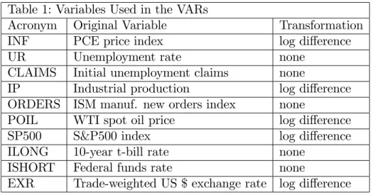
We use data on 10 commonly-used monthly US macroeconomic variables from 1973M1 through 2012M3. All of the data is obtained from the Federal Reserve Bank of St. Louis’ FRED data base. We follow a common practice (see, e.g., Carriero, Clark and Marcellino, 2011) and transform our variables so as to be rates. Table 1 lists our vari-ables and the transformations done. Varivari-ables which were available weekly or daily are averaged to produce monthly …gures. Where relevant, variables are seasonally adjusted. The results below maintain a lag length of 4, but results are relatively insensitive to lag length. In‡ation is the variable common to all VARs (labelled ytf in Section 2), with the remaining variables being potential predictors for in‡ation (labelled yr
t in Section
2).
Table 1: Variables Used in the VARs
Acronym Original Variable Transformation
INF PCE price index log di¤erence
UR Unemployment rate none
CLAIMS Initial unemployment claims none
IP Industrial production log di¤erence ORDERS ISM manuf. new orders index none
POIL WTI spot oil price log di¤erence SP500 S&P500 index log di¤erence ILONG 10-year t-bill rate none
ISHORT Federal funds rate none
EXR Trade-weighted US $ exchange rate log di¤erence
4.2
Which Variables Does DDS Select?
The two main speci…cation choices in DDS are α (which a¤ects the degree of model switching) and κ (which a¤ects the amount of change in Σt). In the following section,
a forecasting exercise will be presented which investigates a wide range of values for α
and κ. However, before doing this, we present evidence on what DDS is doing for the particular choices α = 0.99 and κ = 0.90. The value α = 0.99 is the one suggested by Raftery et al (2010) and κ = 0.90 is a value which allows for a high degree of variation in volatility. As we shall see in the next sub-section, allowing for substantive heteroskedasticity does seem to be important in achieving good forecast performance in this data set.
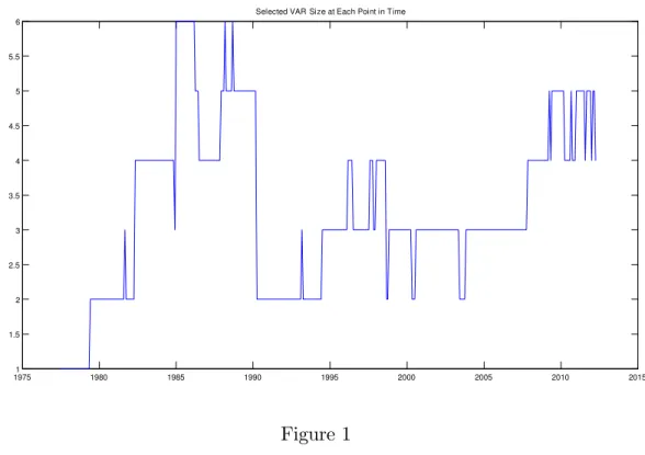
Figure 1 shows the size of the VAR which is chosen by DDS at each point in time. The two main points to note are that DDS is ensuring parsimony and that the VAR dimension switches substantially over time.
On the issue of parsimony, it can be seen that DDS is never choosing a VAR with more than six variables and for most of the time, the dimension is three or less. In fact, for the latter half of the 1970s it is selecting a univariate AR model. Subsequent to the 1970s, the VAR dimension tended to increase in size until an abrupt switch in dimension around 1990. For a long period from 1990 through 2008, DDS chose a three dimensional VAR (occasionally and brie‡y switching to a two or four dimensional model). It is only in the recent recessionary period that the VAR dimension has been increasing. 1975 1980 1985 1990 1995 2000 2005 2010 2015 1 1.5 2 2.5 3 3.5 4 4.5 5 5.5 6
Selected VAR Size at Each Point in Time
Figure 1
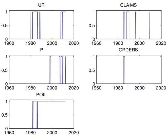
Figures 2 and 3 show which variables DDS has been selecting at each point in time. The numbers in the …gures are “inclusion indicators” which equal one in time periods when DDS is selecting the variable for inclusion in the VAR (and equal zero at other times). The dominant variable is oil price in‡ation which, apart from the late 1970s and a few other brief periods, is selected by DDS. During the period 1990-2008, when DDS
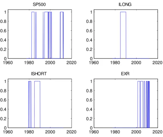
is choosing parsimonious VARs, it is typically using a trivariate VAR involving INF, POIL and SP500. After 2000 (and, in particular, after 2008 when the VAR dimension tends to increase), the exchange rate and unemployment rate also frequently enter as important variables. It is interesting to note that, in the 1980s (when DDS selects VARs with higher dimensions) the long and short term interest rates are included, but subsequently these variables play no role whatsoever. The remaining variables (ORDERS, CLAIMS, IP) only occasionally enter the VAR. Although it is interesting to note that each of these variables is selected at some point in time, indicating they are episodically useful for forecasting in‡ation.
1960 1980 2000 2020 0 0.5 1 UR 1960 1980 2000 2020 0 0.5 1 CLAIMS 1960 1980 2000 2020 0 0.5 1 IP 1960 1980 2000 2020 0 0.5 1 ORDERS 1960 1980 2000 2020 0 0.5 1 POIL
1960 1980 2000 2020 0 0.2 0.4 0.6 0.8 1 SP500 1960 1980 2000 2020 0 0.2 0.4 0.6 0.8 1 ILONG 1960 1980 2000 2020 0 0.2 0.4 0.6 0.8 1 ISHORT 1960 1980 2000 2020 0 0.2 0.4 0.6 0.8 1 EXR
Figure 3: Inclusion Indicators for Individual Variables
4.3
Forecasting Comparison
The preceding sub-section indicates that the VAR dimension is switching over time and that, when forecasting in‡ation, di¤erent variables are useful at di¤erent points in time. In the present sub-section, we investigate whether this switching is leading to substantial improvements in forecast performance. Given that DDS uses the predictive likelihood which evaluates the period ahead forecast performance, we focus on one-period forecasts in this sub-section.
We compare DDS forecast performance to that of several forecasting strategies a researcher might use with VARs of …xed dimensions. In particular, we reason that a researcher might choose one of three strategies: i) use the large VAR (include all 10 variables), ii) motivated by the Phillips curve, use a bivariate VAR for in‡ation and unemployment, or iii) use a univariate AR for in‡ation. In order to make sure our forecast comparison is as fair as possible, we use the same Minnesota priors and same strategy for optimizing the shrinkage parameter in the Minnesota prior in the …xed dimension VARs as we did with DDS. We also allow for heteroskedasticity using the same EWMA estimator as we did with DDS. Homoskedastic variants of the VARs are also treated in the same way for both cases.
We use three standard metrics of forecast performance. Mean squared forecast error (MSFE) and mean absolute forecast error (MAFE) investigate the properties of
the point forecasts of in‡ation. Sums of log predictive likelihoods (LPL) can be used to investigate the forecast performance of the entire predictive density.4 All of these are
evaluated over the period 1977M1 through 2012M3
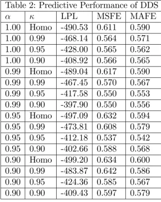
We begin by investigating the sensitivity of DDS to choice of forgetting and decay factors. A strong …nding of Table 2 is that allowing for changes in volatility is important in achieving good forecast performance. Imposing homoskedasticity, or even κ= 0.99, leads to inferior forecast performance relative to values of the decay factor which allow for greater volatility change. This result comes through with moderate strength in the MSFEs and MAFEs. However, it comes through with greater strength in the LPLs which depend not only on the point forecast, but also the predictive variance. This indicates that appropriate modelling of heteroskedasticity is of particular importance in correctly estimating the dispersion of the predictive distribution.
If we ignore the poorly performing homoskedastic and κ= 0.99 rows of Table 2, it can be seen that MSFE and MAFE results are fairly robust to the choice of α. Values of α allowing for a moderate degree of model switching (i.e. α= 0.95or 0.99) tend to perform best, withα= 0.90performing worst. The combinationα= 0.99andκ= 0.90
leads to the best forecast performance as evaluated by LPL. If we use MSFE or MAFE, the combination α = 0.95 and κ = 0.95 forecasts slightly better. But, in general, we are …nding a fair degree of robustness provided we avoid the homoskedastic case and do not allow for too much model switching. Note that, for α= 0.90, forecasts one year ago only receive about 28% as much weight as last month’s forecast performance in the model switching choice. Thus, this value is choosing the forecasting model based only on the very recent past, which is not optimal in the present application.
Table 2: Predictive Performance of DDS
α κ LPL MSFE MAFE 1.00 Homo -490.53 0.611 0.590 1.00 0.99 -468.14 0.564 0.571 1.00 0.95 -428.00 0.565 0.562 1.00 0.90 -408.92 0.566 0.565 0.99 Homo -489.04 0.617 0.590 0.99 0.99 -467.45 0.570 0.567 0.99 0.95 -417.58 0.550 0.553 0.99 0.90 -397.90 0.550 0.556 0.95 Homo -497.09 0.632 0.594 0.95 0.99 -473.81 0.608 0.579 0.95 0.95 -412.18 0.537 0.542 0.95 0.90 -402.66 0.588 0.568 0.90 Homo -499.20 0.634 0.600 0.90 0.99 -483.87 0.642 0.586 0.90 0.95 -424.36 0.585 0.567 0.90 0.90 -409.43 0.597 0.579
4To aid in interpretation, note that sums of log predictive likelihoods over the entire sample will equal the log marginal likelihood. The log Bayes factor is equivalent to the di¤erence in the log marginal likelihoods between two models. There are standard rules of thumb for interpreting Bayes factors (see, e.g., Kass and Raftery, 1995). Also, information criteria such as the Schwarz criterion can be interpreted as approximations to log marginal likelihoods.
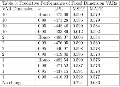
Table 3 presents forecast metrics for the …xed dimension VARs for di¤erent values forκ. As in Table 2, a strong …nding is that allowing for substantial change in volatility is important for achieving good forecast performance as measured by LPL (results for MSFE and MAFE are weaker). However, the most important …nding is that the forecast performance of …xed dimension VARs tends to be substantially worse than DDS. For instance, the MSFEs in Table 3 are rarely much below 0.60. In Table 2, if we ignore the poorly forecasting homoskedastic results, we tend to …nd MSFE values of around 0.55-0.57 (and the lowest MSFE using DDS is 0.537). This represents a 5-10% improvement in forecast performance which, for in‡ation, is substantial. Similarly, in Table 3 the highest LPL is -416.23 which is much lower than the highest LPL of Table 2 which is -397.90. In general, if we compare like with like (e.g. compareκ= 0.95rows in the two tables), you see a deterioration in forecast performance when moving from DDS to the …xed dimension VAR.
The …nal row of Table 3 presents MSFE and MAFE for a no change forecast. These, too, are substantively higher than the ones produced by DDS.
It is also interesting to note that, with …xed dimension VARs, LPLs indicate that the univariate AR model for in‡ation is forecasting best. In contrast, MSFEs and MAFEs show no strong preference for any particular VAR dimension. The fact that DDS is forecasting better (by any of our forecast metrics) and is selecting parsimonious (but rarely univariate) VARs indicate the importance of dimension switching and allowing for di¤erent predictors for in‡ation to enter/leave the VAR over time.
Table 3: Predictive Performance of Fixed Dimension VARs VAR Dimension κ LPL MSFE MAFE
10 Homo -475.66 0.590 0.579 10 0.99 -473.28 0.586 0.579 10 0.95 -448.46 0.599 0.584 10 0.90 -433.89 0.612 0.592 2 Homo -485.07 0.605 0.584 2 0.99 -476.05 0.599 0.580 2 0.95 -440.97 0.598 0.578 2 0.90 -419.80 0.596 0.578 1 Homo -482.54 0.599 0.576 1 0.99 -471.52 0.587 0.576 1 0.95 -437.15 0.594 0.578 1 0.90 -416.23 0.592 0.577 No change – – 0.724 0.636
These empirical results show the computational feasibility and usefulness of DDS in a VAR of up to 10 dimensions on a standard personal computer. Extensions to VARs somewhat larger than this (e.g. 15 or 20 dimensions) could be handled if a faster computer were used or the researcher was willing to tolerate a greater computation time. However, in the near future, it is unlikely that DDS as implemented in this paper could be done using large VARs involving 100 or more variables (such as the one in Banbura et al, 2010). Even a very fast computer would take many years to evaluate250
or2100VARs. In such a case, we would recommend restricting the model space in some
dimension. Or the researcher may wish to divide variables into blocks (e.g. a …nancial block, a monetary block, etc.) and consider only VARs which select one variable from each block.
In our empirical work, the goal was to investigate the performance of DDS for a range of forgetting and decay factors. It is worth noting that it is also possible (at some computational cost) to estimate these factors. The interested reader is referred to McCormick, Raftery, Madigan and Burd (2012) and Koop and Korobilis (2012).
5
Conclusions
When working with Bayesian VARs, parsimony is often a concern. When forecasting, the researcher is often concerned with whether the set of variables useful for forecasting is changing over time. In this paper, we have developed DDS methods which address both these concerns. DDS can be used to choose VAR dimension and, in addition, allows the dimension of the VAR to switch over time. The results of an in‡ation forecasting exercise suggest that DDS is a potentially useful addition to the Bayesian VAR toolbox.
References
Andersson, M. and Karlsson, S. (2009). “Bayesian forecast combination for VAR models,” pages 501-524 in S. Chib, W. Gri¢ths, G. Koop and D. Terrell (eds.),Advances in Econometrics, Volume 23, Emerald Group: Bingley, UK.
Banbura, M., Giannone, D. and Reichlin, L. (2010). “Large Bayesian vector autore-gressions,” Journal of Applied Econometrics, 25, 71-92.
Carriero, A., Clark, T. and Marcellino, M. (2011). “Bayesian VARs: Speci…cation choices and forecast accuracy,” Working Paper 1112, Federal Reserve Bank of Cleveland. Carriero, A., Kapetanios, G. and Marcellino, M. (2009). “Forecasting exchange rates with a large Bayesian VAR,” International Journal of Forecasting, 25, 400-417.
Del Negro, M. and Schorfheide, F. (2011). “Bayesian macroeconometrics,” pages 293-398 in J. Geweke, G. Koop, and H. van Dijk (eds.), The Oxford Handbook of Bayesian Econometrics, Oxford University Press: Oxford.
Ding, S. and Karlsson, S. (2012). “Model averaging and variable selection in VAR models,” manuscript.
Doan, T., Litterman, R. and Sims, C. (1984). “Forecasting and conditional projec-tion using realistic prior distribuprojec-tions,” Econometric Reviews, 3, 1-144.
Fagin, S. (1964). “Recursive linear regression theory, optimal …lter theory, and error analyses of optimal Systems,” IEEE International Convention Record Part i, 216-240. Giannone, D., Lenza, M., Momferatou, D. and Onorante, L. (2010). “Short-term in‡ation projections: a Bayesian vector autoregressive approach,” ECARES working paper 2010-011, Universite Libre de Bruxelles.
Jarocinski, M. and Mackowiak, B. (2011). “Choice of variables in vector autoregres-sions,” manuscript.
Jazwinsky, A. (1970). Stochastic Processes and Filtering Theory, New York: Acad-emic Press.
Karlsson, S. (2012). “Forecasting with Bayesian Vector Autoregressions,” prepared for the Handbook of Economic Forecasting, Volume 2.
Kass, R. and Raftery, A. (1995). ”Bayes factors,”Journal of the American Statistical Association, 90, 773-795.
Koop, G. and Korobilis, D. (2009). “Bayesian multivariate time series methods for empirical macroeconomics,” Foundations and Trends in Econometrics, 3, 267-358.
Koop, G. and Korobilis, D. (2012). “Large time-varying parameter VARs,” manu-script available through http://personal.strath.ac.uk/gary.koop/research.htm.
Korobilis, D. (2012). “VAR forecasting using Bayesian variable selection”, Journal of Applied Econometrics, forthcoming.
Litterman, R. (1986). “Forecasting with Bayesian vector autoregressions – Five years of experience,” Journal of Business and Economic Statistics, 4, 25-38.
McCormick, T., Raftery, A., Madigan, D. and Burd, R. (2012). “Dynamic logistic regression and dynamic model averaging for binary classi…cation,” Biometrics, 68, 23-30.
Raftery, A., Karny, M. and Ettler, P. (2010). “Online prediction under model uncer-tainty via dynamic model averaging: Application to a cold rolling mill,”Technometrics, 52, 52-66.
RiskMetrics (1996). Technical Document(Fourth Edition). Available at http://www. riskmetrics.com/system/…les/private/td4e.pdf.
West, M. and Harrison, J. (1997). Bayesian Forecasting and Dynamic Models, sec-ond edition, Springer: New York.