2006
New statistical methods in bioinformatics: for the
analysis of quantitative trait loci (QTL),
microarrays, and eQTLs
Rhonda DeCook
Iowa State UniversityFollow this and additional works at:https://lib.dr.iastate.edu/rtd
Part of theBioinformatics Commons, and theStatistics and Probability Commons
This Dissertation is brought to you for free and open access by the Iowa State University Capstones, Theses and Dissertations at Iowa State University Digital Repository. It has been accepted for inclusion in Retrospective Theses and Dissertations by an authorized administrator of Iowa State University Digital Repository. For more information, please [email protected].
Recommended Citation
DeCook, Rhonda, "New statistical methods in bioinformatics: for the analysis of quantitative trait loci (QTL), microarrays, and eQTLs " (2006).Retrospective Theses and Dissertations. 1504.
for the analysis of quantitative trait loci (QTL),
microarrays, and eQTLs
by
Rhonda DeCook
A dissertation submitted to the graduate faculty
in partial fulfillment of the requirements for the degree of
DOCTOR OF PHILOSOPHY
Major: Statistics
Program of Study Committee: Dan Nettleton, Major Professor
Alicia Carriquiry Ranjan Maitra Stephen Vardeman
Stephen Howell
Iowa State University
Ames, Iowa
2006
INFORMATION TO USERS
The quality of this reproduction is dependent upon the quality of the copy submitted. Broken or indistinct print, colored or poor quality illustrations and photographs, print bleed-through, substandard margins, and improper alignment can adversely affect reproduction.
In the unlikely event that the author did not send a complete manuscript and there are missing pages, these will be noted. Also, if unauthorized copyright material had to be removed, a note will indicate the deletion.
UMI
UMI Microform 3229065Copyright 2006 by ProQuest Information and Learning Company. All rights reserved. This microform edition is protected against
unauthorized copying under Title 17, United States Code.
ProQuest Information and Learning Company 300 North Zeeb Road
P.O. Box 1346 Ann Arbor, Ml 48106-1346
Graduate College Iowa State University
This is to certify that the doctoral dissertation of
Rhonda DeCook
has met the dissertation requirements of Iowa State University
Major Professor
For the Major Prog m Signature was redacted for privacy.
TABLE OF CONTENTS
ACKNOWLEDGEMENTS vii ABSTRACT 1 GENERAL INTRODUCTION 3 1 QTL Analysis 4 1.1 Background 41.2 Genotyping Marker Loci 7
1.3 Experimental Populations in Interval Mapping 8
1.4 Expected Genotypes at Unobserved Loci 9
2 Affymetrix GeneChip Array Technology 15
3 Multiple Testing Adjustment Procedures 18
3.1 For QTL Analysis 19
3.2 For Microarray Analysis 20
4 Dissertation organization 21
5 References 23
6 Glossary 25
CHAPTER 1. QTL DETECTION FOR ZERO-INFLATED POISSON
TRAITS 27
1 Introduction 28
2 Method for Detecting ZIP QTLs 31
2.1.1 Single ZIP Distribution 31
2.1.2 Complete-Data Likelihood for Single ZIP 32
2.1.3 Mixture of ZIP Distributions 33
2.1.4 Complete-Data Likelihood for Mixture of ZIPs 36
2.2 EM Algorithm 38
2.2.1 Background 38
2.2.2 E-step 41
2.2.3 M-step 44
2.3 EM Convergence 45
2.4 Asymptotic Distribution of MLE 48
2.5 Estimating the Asymptotic Variance-Covariance Matrix When Us
ing the EM Algorithm 48
2.6 Genome-wide Test for Existence of QTL 50
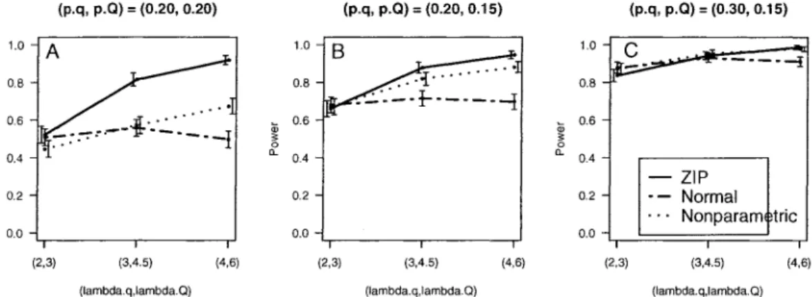
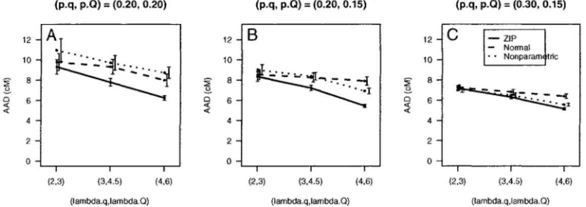
3 Simulation Study 51
3.1 Design 52
3.2 Results 53
3.2.1 Power and Estimated Location of QTL 54
3.2.2 Estimated Parameters at Detected QTL 57
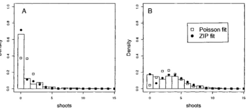
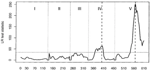
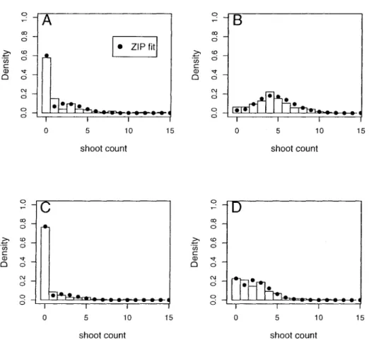
4 Example: Shoot Regeneration Study 62
4.1 Design 62
4.2 Results 63
5 Appendix 67
5.1 Asymptotic Distribution of MLE 67
5.2 Continuity of Q((f)\4>*) in (p and <fi* 77
CHAPTER 2. IDENTIFYING DIFFERENTIALLY EXPRESSED GENES IN UNREPLICATED MULTIPLE-TREATMENT MICRO ARRAY
TIMECOURSE EXPERIMENTS 81
1 Introduction 82
2 Method for Detecting Differential Expression 85
2.1 Notation and Hypotheses 85
2.2 Model Selection 86
2.3 Test Statistic and P-values 87
3 Simulation Study 89
3.1 Design 90
3.2 Results 92
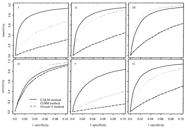
3.2.1 Receiver Operating Characteristic (ROC) curves .... 92
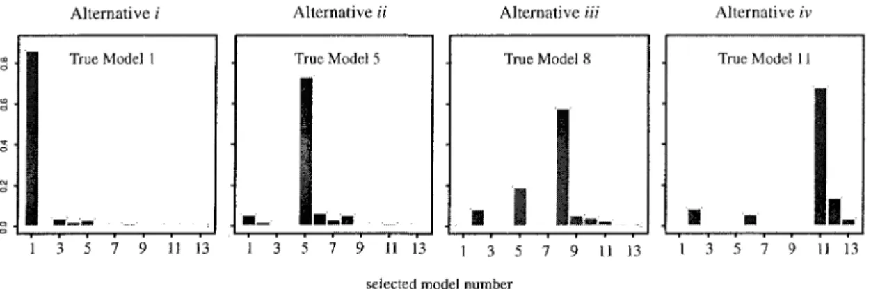
3.2.2 Model choice 95
4 Example: Arabidopsis Experiment 97
5 Related Work 98
6 Discussion 101
7 References 104
CHAPTER 3. GENETIC REGULATION OF GENE EXPRESSION
DURING SHOOT DEVELOPMENT IN ARABIDOPSIS THALIANA 106
1 Introduction 107
2 Materials and Methods 109
3 Results 112
3.1 Single Feature Polymorphisms 112
3.2 Gene Expression Pattern Signatures 114
3.3 Genome Scan 115
4 Discussion 126
5 References 129
CONCLUSIONS AND FUTURE WORK 133
1 Conclusions 133
ACKNOWLEDGEMENTS
For the many hours my major professor, Dr. Dan Nettleton, has spent giving me
guidance and advice, I am incredibly grateful. Through years of weekly meetings and
talks with Dan, I have not only broadened my statistical knowledge, but I feel I have
observed how to be an encouraging and productive professor, something I hope to carry
with me into my own professional career.
I would also like to thank Dr. Alicia Carriquiry for her endless optimism and energy
that she gives so freely to her students. I had the pleasure of working with Alicia during
my time in the Preparing Future Faculty program, and I hope that our friendship will
continue to grow in the years to come.
Finally, I thank my family and friends for all their support. I feel incredibly lucky
to have had such a wonderful group of people to lean on while finishing my graduate
work. But above all, I thank my husband Howard for the patience, understanding, and
ABSTRACT
This thesis focuses on new statistical methods in the area of bioinformatics which
uses computers and statistics to solve biological problems. The first study discusses a
method for detecting a quantitative trait locus (QTL) when the trait of interest has a
zero-inflated Poisson (ZIP) distribution. Though existing methods based on normality
may be reasonably applied to some ZIP distributions, the characteristics of other ZIP
distributions make such an application inappropriate. In this study, we propose a QTL
detection method, appropriate for any ZIP trait, that utilizes the EM algorithm to com
pute maximum likelihood estimates for the ZIP parameters. We compare our method to
an existing non-parametric approach using simulation. The method is illustrated using
QTL data collected on two ecotypes of the Arabidopsis thaliana plant where the trait of
interest is shoot count.
The second study discusses a method to detect differentially expressed genes in an
unreplicated multiple-treatment microarray timecourse experiment. In a two-sample
setting, differential expression is well defined as non-equal means, but in the present
setting, there are numerous expression patterns that may qualify as differential expres
sion. By defining differential expression as any pattern other than a concurrent flat line
over time for all treatment groups, we propose a method that allows the researcher to
test the null hypothesis of no differential expression at every gene. This method pro
vides the researcher with a list of significant genes, an associated false discovery rate
for that list, and a 'best model' choice for every gene. The model choice component
one specific alternative expression pattern. In fact, in this type of experiment, there
are many possible expression patterns of interest to the researcher. Using simulations,
we provide information on the specificity and sensitivity of detection under a variety of
true expression patterns using receiver operating characteristic curves. The method is
illustrated using an Arabidopsis thaliana microarray experiment with five time points
and three treatment groups.
The third study discusses a new type of analysis, called eQTL analysis. This anal
ysis brings together the methods of microarray and QTL analyses in order to detect
locations on the genome that control gene expression. These controlling loci are called
expression QTL, or eQTL. Locating eQTL can help researchers uncover complex net
works in biological systems. For data sets containing thousands of genes and hundreds of
markers, there are potentially millions of tests of interest. Besides the difficulty involved
in sifting through millions of tests, the issues previously discussed in QTL analysis and
microarray analysis are also present here. For each of these types of analysis, a different
multiple-testing adjustment is utilized. The adjustment for a QTL analysis accounts
for the strong correlation between tests at consecutive markers, while the adjustment
for a microarray experiment accounts for the block-structure correlation between gene
expression values in an individual arising from gene coregulation and other gene-to-gene
relationships. Both of these types of multiple testing must be considered when deter
mining statistical significance of eQTLs. The method is illustrated using an Arabidopsis
GENERAL INTRODUCTION
The field of statistics is dynamic in that new methods are continually being de
veloped. These new methods arise from a variety of motivations. For example, the
discovery of better estimators, more efficient algorithms, or advances in technology can
all motivate new methods. The new methods in this thesis are motivated by the new
technology of microarrays, and the search for a more appropriate method in the area of
quantitative trait locus (QTL) analysis. Specifically, we propose a method to locate a
QTL when the trait of interest follows a zero-inflated Poisson (ZIP) distribution. Much
research has been done for normally distributed QTL traits, but traits following other
distributions have received much less attention. Applying existing QTL analysis meth
ods, based on normality, to a ZIP trait provides less information than our proposed
method, and in many cases, is even inappropriate. Second, we propose a method to
detect differentially expressed genes in an unreplicated multiple-treatment microarray
timecourse experiment. The analysis of this type of microarray data challenges the
statistician because it must incorporate a model selection procedure and a differential
expression testing procedure at each of thousands of genes simultaneously. Finally, QTL
analysis and microarray analysis are joined together to detect eQTL, or expression-level
quantitative trait loci. In this emerging area of research, gene expression is considered
the quantitative trait of interest. Thus, there are thousands of traits on which to perform
QTL analysis. Because any gene may be controlled by any location, there are poten
tially millions of gene-to-locus tests of interest. Just sifting through the vast number of
correlation in tests performed on consecutive chromosome locations on the genome.
The new methods proposed in this dissertation are all applied to data from the fields
of genetics and biology. This introduction includes some background information on
QTL analysis, microarrays, and related terminology. We also include some background
on statistical procedures to adjust for multiple testing because procedures of this type
are utilized for both QTL and microarray analyses.
1 QTL Analysis
1.1 Background
The intentional breeding of organisms to produce offspring with desirable charac
teristics, or traits, is an old and common practice. Successful breeding relies on the
existence of an association between an observed trait and the genetic composition of the
organism. The simplest association occurs when a trait is linked to a single locus on the
genome. This describes a trait with single-locus control, otherwise known as a simple
trait. For such a trait, we often find that much of the variability in the observed trait
can be explained by the controlling locus genotype. More complex associations exist
when a trait is linked to many loci on the genome. For these associations, the genotypes
at the given loci work together to control the observed trait. This type of trait is called
a complex trait. It is the discovery of either type of these associations that is the goal
when performing quantitative trait locus (QTL) analysis.
With advances in technology, we can now determine the genotype (i.e. specific DNA
sequence) an individual possesses at particular locations throughout the genome. QTL
analysis applies statistical modeling to a data set containing information on location
genotypes and an observed trait to search for potential controlling loci of the trait. The
containing the gene controlling the trait of interest. A gene is defined here as DNA
that encodes for a protein or any RNA used in an organism's biological system. Many
organisms, including humans, are diploid and their nucleus contains two copies of each
gene, except for the genes in human males residing on the sex chromosomes. Each copy
of a gene can take on any one of a number of DNA codings called alleles. Thus, at any
locus on the genome, a pair of alleles defines the genotype at a gene. Letters are often
used to represent alleles, such as B or b, and the combination of alleles define the geno
type, such as BB, Bb, or bb at a given locus. When alleles differ at a given locus in a
population, the locus is said to be polymorphic. Such loci are the subject of population
genetic studies (Lynch and Walsh, 1998). We can also extend the concept of polymor
phisms to DNA not in genes, sometimes referred to as non-coding regions. Thus, with
infinite time and money, every DNA polymorphism in the genome could be genotyped.
In reality, the number of known polymorphisms along the genome of an organism may
be small, often in the hundreds. However, in some organisms, including man, thousands
of polymorphisms have been identified. We refer to the DNA polymorphisms used in
our QTL analysis as markers (see next section).
As the ability to genotype individuals progresses, so does our ability to associate
traits of interest with specific genes on the genome. A QTL is a section of DNA con
taining the gene associated with a quantitative trait. When a QTL exists, the trait of
interest is associated with the genotype at the controlling locus. As each QTL geno
type is associated with a distinct trait distribution, we model the marginal distribution
of observed traits as a finite mixture distribution. In this mixture model, each QTL
genotype is associated with one component of the mixture. QTL experiments are often
designed using experimental organisms or populations with very few possible genotypes
at each genome position. For example, by backcrossing the offspring of parental inbred
lines with one of the parents we can produce organisms with only two possible geno
also apply to populations with more than two genotypes at each locus, which is more
common in nature.
Traditional QTL analysis provides us with a likelihood-ratio (LR) test statistic for
each genome position tested. The null hypothesis is that the tested location is not a
QTL. The number of locations tested depends on how many locations the researcher
chooses to test. If the researcher chooses to test for a QTL only at observed locations
(markers), they can perform single marker analysis. But if the researcher wants to test
for QTL at more locations, they can use interval mapping to test for QTL at unobserved
locations between markers. A researcher may choose to apply interval mapping when the
data set has a relatively sparse set of markers. Testing at more locations provides greater
precision in detecting the QTL, but increases computation time. The information in the
set of LR tests, one test for each location, is usually summarized using a plot showing
genome location on the horizontal axis versus the LR test statistic on the vertical axis.
The position with the largest LR test statistic shows the strongest evidence for being a
QTL, but determining whether this finding is statistically significant requires applying
a multiple testing adjustment.
As a final note in this QTL background section, even when a genome location tests
as statistically significant for being a QTL, there is usually more work to be done. The
testing position showing the greatest evidence for the presence of a QTL is not actually
associated with an exact physical location on the genome. The location of the testing
position is commonly defined in terms of centiMorgans, which is a genetic distance based
on recombination fractions (see Section 1.4), rather than a physical distance measured in
kilobases. This centiMorgan position does not necessarily translate directly into a spe
cific physical location, rather it is associated with a region on the genome. Therefore,
once a statistical analysis finds evidence for the existence of a QTL, the researcher must
then search the region associated with the given testing position for the actual QTL.
phism exists. Such a polymorphism is expected to be present because the DNA sequence
at the QTL determines trait group membership, and therefore the sequence should con
tain a categorizing feature (i.e. a polymorphism). Though we know each marker locus
is polymorphic, we do not know ahead of time about the polymorphic state of locations
between markers. To locate the QTL, the biologist must undertake the labor-intensive
process of searching the genome for a candidate gene containing a polymorphism using
available databases and sequencing information. A better statistical estimate for the
QTL position (i.e. closer proximity to the true QTL) can equate to reduced time in
follow-up work for the researcher. Unfortunately, translating the behavior of the QTL
estimate into a confidence interval for the true QTL without applying strict, and per
haps questionable, assumptions is difficult. See Manichaikul et al. (2006) for a recent
comparison of commonly used QTL confidence interval methods.
1.2 Genotyping Marker Loci
In order to genotype marker locations on the genome, we need to identify locations
where a polymorphism exists, and then genotype the given location for each individual.
A common approach to genotyping utilizes restriction enzymes that cut DNA when a
specific sequence of nucleotides is present. A site that gets cut is called a restriction site
and is often 4 to 6 nucleotide-bases long. Two restriction enzymes associated with two
restriction sites in close proximity can cut the DNA and create a relatively short DNA
fragment composed of the DNA that was between sites. When a polymorphism exists
between two DNA strands, application of these two enzymes to the DNA strands can
produce fragments of differing lengths. For instance, if one strand has an insertion of
nucleotides between restriction sites, its fragment length will be longer than the strand
without the insertion. This difference is called a Restriction Fragment Length Polymor
organisms. An RFLP can also arise when a mutation creates or destroys a restriction
site (Lynch and Walsh, 1998).
In practice, DNA is digested with a variety of restriction enzymes at one time. When
the digested DNA is run on a gel under an electric current, fragments of differing lengths
will travel different distances. Thus, the fragments will group by size. With so many
RFLPs represented on the gel, the groupings are not clear and rather uninformative.
Thus, labeled DNA probes are used to identify particular regions of the DNA for marker
analysis. Each probe represents a marker, and the differing alleles for the marker appear
at distinct locations on the gel. This procedure can be done for each individual. There
are also other techniques that can highlight several DNA fragments at a time such as
Randomly Amplified Polymorphic DNAs (RAPDs). See Lynch and Walsh (1998) for
more background on molecular markers.
1.3 Experimental Populations in Interval Mapping
Various mapping populations commonly used in QTL studies are backcross popu
lations, intercross populations, and recombinant inbred line populations. These pop
ulations are valuable for QTL studies because we know the breeding structure under
which they were propagated, and this structure provides linkage disequilibrium within
the propagated individuals (Liu, 1989). Linkage disequilibrium (LD) exists when cer
tain combinations of alleles at numerous genome locations occur more frequently than
others. LD occurs because genetic material from each chromosome tends to be inher
ited in sections, so the alleles at locations in close proximity will tend to be inherited
together. The existence of linkage disequilibrium is what allows us to search for QTL
locations between observed markers. The small number of possible genotypes at each
genome locus in these populations also make them easy to deal with in terms of model
at every loci) of a particular species that differ for the trait of interest. We will refer
to these as the parental lines and refer to their respective genotypes as AA and BB.
Crossing the two parental lines generates an F% population that has an AB genotype
at every locus. By crossing this Fi population with one of the parental lines we can
produce a backcross population. For example, crossing an Fj organism with the AA
parent produces an organism with either an AA or an AB genotype at each locus. The
determining factor on whether an AA or AB genotype is present depends on the fre
quency and location of crossover events during the meiosis phase of reproduction (see
next section). Intercross populations are developed by crossing the F% population with
itself. An organism in an intercross population has one of three possible genotypes at
each loci, AA, AB, or BB in this example. Finally, a recombinant inbred line population
is developed by first producing an Fi population from the parental lines, then repeatedly
self-crossing the Fi organisms until eventually, new homozygous lines are created that
have either an AA or BB at each locus. These new lines are called recombinant inbred
lines (RILs). In general, RIL populations are advantageous because they tend to have
a large frequency of recombination events across the genome compared to the backcross
or intercross populations. This provides more precision for detecting the location of a
QTL on the genome. RILs are also advantageous in genetics studies because they are
inbred and we can obtain many individuals with the same genotype.
1.4 Expected Genotypes at Unobserved Loci
In interval mapping for experimental organisms, we use the genotypes at observed
loci to place a probability distribution on the genotype at an unobserved location on the
same chromosome. Besides conditioning on observed loci, this probability distribution
is conditional on the probability of a crossover event occurring between the observed
of sexual reproduction. During meiosis, the group of four chromatids composed of the
two sister chromatids from each parent become close enough in proximity that they can
actually exchange genetic material. Crossovers lead to recombinant gametes that have
a genetic sequence different from that found in the parental chromatids (provided par
ents were not inbred and homozygous before mating). Such recombination of gametes
contributes to genetic variability in a population as a whole.
The occurrence of crossover events on the genome can be modeled as a Poisson
process. Consider the full length of the genome formed by sequentially placing the chro
mosomes end to end. We define one end of the genome to be positioned at the origin
of a 1-dimensional axis. As one moves along the genome, the distance from the origin
increases. We define Xd as the number of crossover events occurring between the origin
and the position located at a distance d from the origin. Then, {xj : d 6 D} for the set
of increasing genome positions D = {d1:d2,...} is a stochastic process. The distance
between two crossover events can modeled as an exponential(A) random variable (pa
rameterized such that the expected distance between events is 1 /A). Assuming there
is no crossover interference1 (i.e. the occurrence of a crossover doesn't inhibit another
crossover occurring nearby), the distances between events across the full genome are all
independently and identically distributed with this exponential(A) distribution. Given
this independence, the number of crossover events occurring at a distance d from the
origin is modeled as a Poisson random variable with an expected number of dX events.
This Poisson(dA) distribution arises out of the relationship between the gamma distri
bution (from the relevant sum of independent exponential random variables) and the
Poisson distribution. The parameter A itself is associated with the expected number of
crossover events between the origin and the position at 1 distance unit from the origin.
The unit of measurement for distance along the chromosome is called the Morgan (M),
*No crossover interference is commonly assumed, but there is some evidence that crossover events are not uniformly distributed along a chromosome. For example, centromeres and telomeres tend to have lower frequencies of crossover events
and is defined as the distance in which the expected number of crossovers is 1. Thus,
the rate parameter À is 1 when using the Morgan as the distance measure, as we do
in this paper. Finally, as the exponential distribution has the 'memoryless' property,
the number of crossover events occurring between locations at a distance rfj and dj with
j > i is Poisson distributed with an expected number of (dj — di) crossovers.
The Poisson process model now gives us a connection between the number of crossover
events occurring between two loci on the genome and the length (in Morgans) of the
interval formed by the loci. This implies that if we could observe crossover events in
any interval, we could also estimate the distance between the loci forming the interval.
Unfortunately, crossover events are not directly observable in experimental organisms be
cause we do not genotype the full genome, only certain markers. The genotypes present
at markers do give us some information on the frequency of crossovers. For example,
consider the backcross population described in Section 1.3 above where each genome
locus can be coded as either 0 or 1. Two markers on a chromosome forming an interval
can be coded as (0,0), (0,1), (1,0), or (1,1). If we observe a (0,1) or (1,0), we say a re
combination event has occurred between the loci. In this situation, we know that an odd
number of crossover events have taken place between the loci. Similarly, if we observe
a (0,0) or a (1,1) at the two locations, then we know an even number (including zero)
of crossover events has occurred. In a genotyped sample, the fraction of the organisms
showing a (0,1) or (1,0) marker configuration is defined as the estimated recombination
fraction between the two markers. This recombination rate between markers is tradition
ally symbolized by 0 and represents the probability of a recombination event occurring
between the two loci.
Using the Poisson process model described above, we can model the probability of
a recombination event occurring as the probability that an odd number of crossover
events has occurred. Thus, letting m = t — s represent the distance in Morgans between
s has a Poisson(m) distribution, and
9 = f (recombination event)
= f (an odd number of crossover events)
= 1 — f (an even number of crossover events)
e~mm(2y)
=
= 1-e-(e'"+2e""'
= \ (1 " e-2m) •
This relationship between 6 and m is known as Haldane's mapping function, and it
allows us to convert from a Morgan distance to a recombination rate. By inverting
the above equation, we form the function converting a recombination rate (estimated
through observed marker genotypes) to a Morgan distance, shown as
m = —0.51og(l — 29).
In the context of QTL interval mapping, we focus our attention on three particular
locations. These locations represent a left marker L, a right marker R, and a putative
QTL location Q between the markers. We let mLR represent the genetic distance between
L and R, mLQ represent the genetic distance between L and Q, and mQR represent
the genetic distance between Q and R. We also let 9 represent the recombination rate
between markers L and R, rL represent the recombination rate between L and Q, and
rR represent the recombination rate between Q and R. As additivity of genetic distance
holds, we have
^LR = mLQ "t" mQK
—0.51og(l — 29) = — 0.51og(l — 2rL) H—0.51og(l — 2rR)
and after reducing the equation, we get
9 = rL + rR - 2rLrR.
This relationship between the three recombination rates is sometimes utilized to simplify
formulas as any one of the three can be written in terms of the other two.
As is apparent from the Poisson process for modeling, there is a higher probability of
a recombination between loci that are farther apart than those that are closer together.
This behavior plays a role in trying to predict the genotype of an unobserved locus that
falls between two observed loci. For example, consider again a backcross organism that
has two loci very close together with the first locus coded as a 0 and the second locus also
coded as a 0. Because the chance for a crossover event occurring between the loci is very
small, any location between the two loci is probably also a 0. If the two observed loci
had been 0 and 1, we know that a crossover event occurred somewhere in the interval,
and so we are less certain about the predicted genotype for any locus between the loci.
Continuing with the backcross scenario, we now look at estimating genotypes at un
observed loci. Let xleft and xright be the observed marker genotypes at markers flanking
a given genome interval. A putative QTL location between these markers is specified
using the parameters 9, rL, and rR as defined above. Each of these recombination frac
tions can be converted into a genetic distance, thus specifying the genome location (in
Morgans) of the putative QTL. Using these recombination fractions, we can compute
the probability that the putative QTL location has a genotype of 0 or 1 conditional on
Table 1
Conditional probabilities of putative QTL genotype
given observed flanking markers in a backcross population.
Marker Conditional probability of
genotype QTL genotype *^left ^right 0 1 0 0 0 1 (l-rL)(l-m) rLrR 1-0 1-9 (l-rL)rR rL(l-rR) e e 1 0 rL(l-rR) e (l-re L)rR 1 1 r-L»"R 1-6» (l-rL)(l-rR) 1-6»
The denominators in the Table 1 probabilities all contain 6 and reflect the condi
tioning on what has been observed in the markers. The recombination fractions used
in practice tend to be small, and markers are usually measured in centiMorgans (cM)
rather than Morgans. Using Haldane's mapping function, we see that two loci at lcM
apart have a recombination fraction of ~ 0.01. This suggests that when we observe the
genotypes at these markers in 100 individuals, we expect, on average, 1 of the individ
uals to exhibit a recombination event. When markers are close together (i.e. rL and rR
are very small) and no recombination has been observed, we can see in Table 1 that it
is much more likely that any locus between the markers is the same genotype as the
markers themselves. For such a locus to have a different genotype than the markers, an
even number of crossover events greater than 0 would have had to occur between the
markers.
In QTL analysis, we utilize the probability that a putative QTL is a specific geno
type given the observed flanking markers. When there are only two possible genotypes,
as in the backcross scenario, we can consider the QTL genotype as a binary random
dom variable equals 1. Using the information in Table 1, we now write the proba
bility that the putative QTL=1 for individual i as a function g of marker genotypes
= (ziLiZia) = (%i i.a, alight), and QTL location:
7r(%«;#,rL,rR) = f (QTZ, =
As this thesis focuses on populations with two possible genotypes, we will use this func
tion iï(Xi\9, rL, rR) in subsequent chapters as part of our mixture modeling notation and
associated likelihoods.
2 Affymetrix GeneChip Array Technology
Microarray technology is used for measuring gene expression in an organism. After
a gene is 'turned-on', the gene expresses itself by producing protein. The production
of a protein is carried out in two distinct stages called transcription and translation.
During transcription, the genetic information in a DNA sequence, or a gene, is tran
scribed into a complementary sequence called mRNA. The translation process follows
next by translating this mRNA sequence into the protein the original DNA sequence
was coded to produce. Base pairing characteristics of mRNA make it easier to measure
than protein, and microarrays are designed to measure the steady state levels of specific
RNAs at the time of sampling. In essence, we measure RNAs are a surrogate for protein
measurement.
The key to measuring mRNA levels on a microarray is the complementary base-pair
structure inherent in every DNA sequence. The four nitrogen bases that combine to
form DNA are adenine (A), guanine (G), cytosine (C), and thymine (T). Base-pairing
occurs in the double helix structure as G pairs with C, and A pairs with T. mRNA
is a single-stranded complementary copy of one side of an 'unzipped' DNA sequence
composed of similar bases, except that the T is replaced with a U, for uracil. In general,
we can consider each mRNA sequence to be associated with one specific location on the
genome, namely, the location of the gene that produced it. Microarrays are designed to
take advantage of the uniqueness of these mRNA sequences.
To measure expression, we collect a sample from a biological organism that contains
thousands of distinct mRNA sequences. The number of copies of each distinct mRNA
sequence is related to the transcriptional output of the cognate gene and the turnover
rate of the mRNA. When using Affymetrix GeneChip technology, collected mRNA is
converted into a flourescent labeled complementary RNA, or cRNA, and it is this la
beled cRNA sample that is actually placed on the array and measured to determine gene
expression.
A common characteristic for all arrays is that short sequences of DNA represent
ing segments of the genome are attached to the array. Millions of copies of each short
oligonucleotide sequence are attached in one location called a spot or a probe on the
array. When the array is incubated with a solution containing the labeled cRNA, the
cRNA hybridizes to the spot or probe that is complementary to its sequence. The fluo
rescent label allows measurement of the quantity of cRNA present at each spot or probe
by its fluorescence intensity. The procedure provides an intensity measure at each probe
allowing comparison of the relative levels of expression at the same gene across multiple
samples (i.e. across multiple arrays).
The probe sequences can be printed, spotted, or synthesized on the arrays. Probes
can be composed of a few bases (oligonucleotides), or they can be composed of hundreds
of bases (cDNAs). In this thesis, we focus on expression data collected using Affymetrix
GeneChips. In these microarrays, millions of copies of each sequence of interest (25
bases in length called 25-mers) are first covalently attached to the GeneChip through
called a probe. Affymetrix uses a grouping of 11 pairs of probes to represent a gene, and
together these probes form a probe set. Probe synthesis for each probe set on a chip
occurs in parallel, resulting in the addition of an A, C, T, or G nucleotide to multiple
growing chains simultaneously across the whole array (Affymetrix, 2001). A probe pair
has both a 25-mer called the perfect match probe (PM) designed to be complementary
to the reference RNA, and a second 25-mer positioned next to the PM probe on the
chip called the mismatch probe (MM) that is an exact replica of the first except that
the middle base has been intentionally switched with its complementary base, therefore
producing a sequence not naturally occurring in the organism. In theory, the presence
of this MM probe on the microarray allows for a measure of noise in the data (called
non-specific binding) because no cRNA sequence would be expected to correctly attach
itself to a MM probe.
After hybridization, the GeneChip is washed to remove excess cRNA that did not
hybridize to any probes. Then, a staining reaction is performed on the chip to allow a
scanner to quantify the amount of cRNA that hybridized to each probe set. The expres
sion of any gene is represented by values in a 2x11 matrix with one row representing the
PM probe flourescence values, the other row representing the MM probe fiourescence
values, and the columns corresponding to probe pairs. Usually, a summary statistic for
these 22 values is computed in order to perform gene-based statistical analyses, such as
identification of differentially genes.
Numerous probe set summary statistics have been suggested, and much controversy
has arisen in choosing one as a 'best' summary (Choe et al., 2005). Affymetrix provides a
commonly used summary statistic called MAS5.0 (Affymetrix, 2001) that incorporates
Tukey's bi-weight and the values of the MM probes. Another commonly used sum
mary statistic that does not incorporate information from the MM probes is the Robust
Multi-chip Average (RMA) suggested by Irizarry et al. (2003). Similary, other proce
correction, have generated much discussion in the research community. Because this
thesis focuses on statistical issues that arise after the application of these procedures, we
do not attempt to compare these procedures in this paper. Instead, we simply mention
that our proposed methods are applicable to probe-set summary statistics computed
after the researcher applies the relevant procedures of his or her choice.
3 Multiple Testing Adjustment Procedures
Both QTL and microarray analyses generate hundreds, maybe even thousands, of
test statistics from one data set. The process for determining significance for such a
situation is different than when there is only one test of interest. One goal of multiple
testing procedures is to filter a large pool of tests down to a relatively short list of statis
tically significant tests that are associated with a low false positive rate. A second goal
is to maintain a low false negative rate with respect to the tests that were not chosen
for the significance list. Controlling the family-wise error rate (FWER) is a common
approach to control the number of false positives in a multiple-testing scenario. After
choosing a threshold that controls the FWER at a = 0.05, any generated list of signifi
cant tests contains no false positives 95% of the time (i.e. if this procedure were repeated
100 times, only 5 of the 100 lists would be expected to contain one or more false posi
tives). The Bonferroni adjustment can be easily applied to a multiple-testing scenario
to achieve a chosen FWER, but this adjustment tends to be fairly conservative and is
often associated with a high rate of false negatives. For example, when the number of
tests performed is in the thousands, it is very feasible that no test is declared significant
after applying the Bonferroni adjustment. The chosen FWER has been achieved, but an
empty list of significant tests provides no information for further study. Perhaps apply
high, or when very few of the tests are expected to be true positives. But in the case
of QTL and microarray analyses, it is usually thought that at least some, and maybe
even thousands, of the tests are true positives. Also, the significance list in a QTL or
microarray analysis is usually not an end in itself, but rather a springboard for further
biological investigation and verification. Thus, procedures other than the conservative
Bonferroni adjustment, and error rates other than the FWER are often utilized for QTL
and microarray analyses.
3.1 For QTL Analysis
As mentioned in Section 1.1, a researcher performing a QTL analysis chooses (3
locations along the genome at which to test for a QTL. The null hypothesis for each test
is the same, and it states that the the given location is not a QTL. Consecutive tests
along the genome are often strongly correlated. When a genome location coincides with
a large LR test statistic, the locations near it often show evidence of being a QTL as
well due to linkage disequilibrium. This strong dependence in consecutive tests along
the genome must be accounted for in determining significance.
Churchill and Doerge (1994) developed a method for determining significance in
QTL studies that has become widely used. Their method uses permutation to develop
an empirical distribution for the maximum of the /3 test statistics that would be seen
under the null. This empirical null distribution is then compared with the original test
statistics for determining significance at a given FWER. Specifically, to create one null
data set, the trait data is permuted among the individuals while the marker data remains
unchanged (i.e. the genotype for each individual remains unaltered). This null data set
has the same marker dependence structure as the original data, but has no association
between the markers and the trait values. Instead of keeping track of all f3 test statistics
repeating this permutation process N> 1000 times, we have an empirical distribution of
the maximum test statistic under the null. By summarizing the (5 tests into one value, the
issue of dependence between tests has been resolved. Choosing a significance threshold
as the 100(l-a) percentile of the maximum test statistic null distribution controls the
FWER at the a level. The type I error rate holds under minimal assumptions about the
distribution of traits, specifically, that the trait values are exchangeable under the null.
This procedure essentially tests the null hypothesis of no association between the trait
and the full genome map, an experimentwise statement. Rejecting this null suggests
that there is at least one location on the genome that is associated with the trait.
3.2 For Microarray Analysis
The dependence between tests in a microarray analysis arises from the complex re
lationships between genes in a biological system. This type of dependence is inherently
different than the dependence that exists between consecutive markers, and is dealt with
in a different manner. Specifically, the adjustment we use for multiple testing in
microar-rays is appropriate for a block-structure correlation, which is a reasonable structure for
modeling gene correlation. A common microarray analysis is to perform a hypothesis
test for differential expression at each of G genes, with G usually in the thousands or tens
of thousands. By applying a Bonferroni multiple-testing adjustment, we could achieve
a FWER of 0.05 by using a p-value threshold of 0.05/G. But because this method is
quite conservative and researchers are often willing to risk getting a few false positives
in order to decrease the number of false negatives, other methods are usually employed.
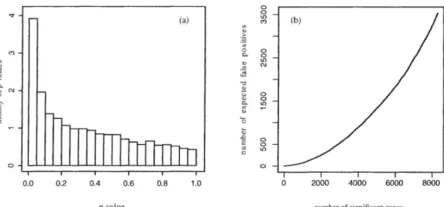
Benjamini and Hochberg (1995) introduced a new approach to multiple testing that
advocated controlling the expected proportion of false positives among all rejected hy
potheses. The motivation for their approach is expressed in their statement:
taken into account and not only the question whether any error was made.
(Benjamini and Hochberg, 1995)
Letting R be the total number of hypotheses rejected and V be the number of false
rejections, they define the false discovery rate (FDR) to be E {j^\R> 0) • P(R > 0).
The inclusion of P(R > 0) is needed because it is not possible to control the conditional
expected value of ^ alone. Specifically, in the case when all tests are true null tests,
the expected value of the proportion, given that any rejections are made, is always 1.
In their paper, they provide a sequential p-value procedure for choosing an appropriate
number of rejections to control this FDR at the a level.
Storey (2002) extended the work of Benjamini and Hochberg by using a different
approach. Instead of using a sequential p-value procedure, he described how to estimate
the FDR once a rejection region F has been chosen. By incrementally changing the re
jection region and recomputing the estimated FDR, a F0 rejection region can be chosen
that coincides with a specific number of significant tests and an acceptable expected
number of false positives. Storey et al. (2003) showed that this method conservatively
and consistently estimates the FDR for all rejection regions simultaneously. In general,
as the number of significant tests increases, so will the FDR. The possible pairs of val
ues from which a researcher can choose depend on the data, and one hopes for a small
increase in the FDR as more tests are designated as significant.
4 Dissertation organization
The three papers in this thesis all relate to the field of bioinformatics. The focus of
the first paper is on the detection of quantitative trait loci. The second paper discusses
the detection of differentially expressed genes in microarray analyses. The third paper
to detect locations of genetic control of gene expression.
The sections of this thesis include an introduction, three research papers, and a con
clusion discussing future work. Chapter 1 discusses the first research paper where we
propose a method to detect a QTL in the case of a zero-inflated Poisson trait. We show
how this method outperforms existing methods based on normality in many situations
using simulations. The EM algorithm is utilized to estimate parameters in the related
likelihood. In Chapter 2, we propose a method to detect differentially expressed genes
in a multiple-treatment microarray timecourse experiment. This type of experiment
presents challenges to the statistician because it incorporates both multiple-testing and
model choice issues. Our method provides both a 'best' model choice, and a p-value
for determining differential expression significance at each of thousands of genes. We
provide information on the specificity and sensitivity of detection under a variety of true
expression patterns using receiver operating characteristic curves. In Chapter 3, we dis
cuss a new type of analysis called eQTL analysis. The goal of this analysis is to detect
loci controlling gene expression at other locations on the genome. These controlling
loci are called expression QTL, or eQTL. For data sets containing thousands of genes
and hundreds of markers, there are potentially millions of tests of interest. Besides the
difficulty involved in sifting through millions of tests, the issues seen in QTL analysis
and microarray analysis are both present. For example, in multiple-testing adjustments,
the type of dependence between tests must be considered. The adjustment for a QTL
analysis accounts for the strong correlation between tests at consecutive markers, while
the adjustment for a microarray experiment accounts for the block-structure correlation
between gene expression values in an individual. Both of these types of multiple testing
must be considered when determining statistical significance of eQTLs. We conclude
5 References
Affymetrix (2002). Microarray Suite User's Guide, Version 5.
Affymetrix, http://www.aSymetrix.com/support/technical/manuals.aSx
Benjamini, Y., and Hochberg, Y. (1995). Controlling the false discovery rate: A prac
tical and powerful approach to multiple testing. J. R. Statist. Soc. B 57, 289-300.
Choe, S.E., Boutros, M., Michelson, A.M., Church, G.M., and Half on, M.S. (2005).
Preferred analysis methods for Affymetrix GeneChips revealed by a wholly defined
control dataset. Genome Biology 6, R16.
Churchill, G.A., and Doerge, R.W. (1994). Empirical threshold values for quantitative
trait mapping. Genetics 138, 963-971.
Irizarry, R.A., Hobbs, B., Collin, F., Beazer-Barclay, Y.D., Antonellis, K.J., Scherf,
U., and Speed, T.P. (2003). Exploration, normalization, and summaries of high
density oligonucleotide array probe level data. Biostatistics 4, 249-264.
Lander, E.S., and Botstein, D. (1989). Mapping mendelian factors underlying quanti
tative traits using RFLP linkage maps. Genetics 121, 185-199.
Liu, B-H. (1998). Statistical genomics: Linkage, mapping, and QTL analysis. CRC
Press, Boca Raton, Florida.
Lynch, M., and Walsh, B. (1998). Genetics and analysis of quantitative traits. Sinauer
Associates, Inc., Sunderland, Massachusetts.
Lockhart, D.J., Dong, H.L., Byrne, M.C., Follettie, M.T., G alio, M.V., Chee, M.S.,
Mittmann, M., Wang, C., Kobayashi, M., and Horton, H. (1996). Expression mon
itoring by hybridization to high-density oligonucleotide arrays. Nature
Manichaikul, A., Dupuis, J., Sen, S., and Broman, K.W. (2006). Poor performance of
bootstrap confidence intervals for the location of a quantitative trait locus. Johns
Hopkins University, Dept. of Biostatistics Working Papers. Working Paper 105.
http://www. bepress. corn/jhubiostat/paper 105
Storey, J.D. (2002). A direct approach to false discovery rates. J. R. Statist. Soc. B
64, 479-498.
Storey, J.D. (2003). Strong control, conservative point estimation and simultaneous
conservative consistency of false discovery reates: a unified approach. J. R. Statist.
5"oc. B 66, 187-205.
Storey, J., and Tibshirani, R. (2003). Statistical significance for genomewide studies.
6 Glossary
allele any one of a number of viable DNA codings of the same gene occupying a given locus on a chromosome.
backcross population offspring generated through a cross between an inbred parent and an F1 organism.
centiMorgan (cM) genetic distance unit of the genome. One crossover event is expected in a genetic distance of 1 Morgan, and 1 Morgan is 100 cM.
centromere a region of chromosome at which sister chromatids are attached during cell division.
crossover exchange of chromosomal genetic material between nonsister
chromatids of homologs during meiosis.
eQTL a section of DNA containing the gene associated with a gene expression trait.
F1 population offspring generated through a cross between two inbred parental lines.
F2 population offspring generated through a cross between F1 organisms.
gene DNA that encodes for a protein or any RNA used in an organism's
biological system.
genotype the specific genetic makeup of an individual, in the form of DNA.
hybridization the process in which a labeled cRNA sample adhere to a microarray according to base-pair complementation.
inbred line population of organisms that are genetically uniform. Breeding within the population produces another genetically identical organism.
interval mapping a procedure used to test for QTL within the interval bound by two marker locations.
interval mapping a procedure used to test for QTL within the interval bound by two marker locations.
kilobase (kb) physical distance unit of the genome. Unit of length for DNA fragments equal to 1000 nucleotides.
linkage disequilibrium describes a situation in which some combinations of alleles or genetic markers on a chromosome occur more frequently in a population than would be expected under independence between the locations.
a section of double-stranded deoxyribonucleic acid (DNA).
a known DNA sequence that can be identified in an organism by a simple assay.
(cM) genetic distance unit of the genome. One crossover event is expected in a genetic distance of 1 Morgan, and 1 Morgan is 100 centiMorgans.
RNA that encodes and carries information from DNA during transcription to sites of protein synthesis to undergo translation in order to yield
a gene product.
oligonucleotide short sequences of nucleotides (RNA or DNA), typically with twenty or fewer bases.
polymorphism different, detectable alleles for a gene or marker in a population.
QTL a section of DNA containing the gene associated with a
quantitative trait.
restriction fragment length polymorphisms (RFLP) an assay in which organisms may be differentiated by analysis of patterns derived from cleavage of their DNA. Used to genotype markers.
telomere DNA at ends of chromosome. locus
marker
Morgan
CHAPTER 1. QTL DETECTION FOR ZERO-INFLATED
POISSON TRAITS
A paper to be submitted to Biometrics
Rhonda DeCook and Dan Nettleton
Abstract
Much work has been done on detecting QTLs when the trait of interest is normally
distributed. This paper presents a method for detecting QTLs for zero-inflated Poisson
(ZIP) traits. A few non-normal trait distributions have received some attention in the
area of QTL analysis. Methods for binary, ordinal, and Poisson traits have been pro
posed, but many other non-normal traits have yet to be investigated. Though existing
methods based on normality may be reasonably applied to some ZIP distributions, the
characteristics of other ZIP distributions make such an application inappropriate. The
method proposed in this paper is appropriate for any ZIP distribution. Using simula
tion, we compare our method to two existing applicable approaches. The method is
illustrated using QTL data collected on two ecotypes of the Arabidopsis thaliana plant
1 Introduction
A quantitative trait locus (QTL) is a locus on the genome that contributes to a
phenotype that varies quantitatively. In general, the alleles present at such a locus are
thought to play a role in determining the level of the quantitative trait. The genetic
mapping of QTLs gives insight into the genetics behind observed traits and can help
advance genetic research on the trait of interest. For example, detecting QTLs associ
ated with a disease can provide useful information for developing therepeutic drugs. For
desirable traits, such as high yield in corn plants, detecting QTLs can provide useful
information for selective breeding.
In order to quantify the association between a trait and a putative QTL location, we
need information on the alleles, or genotypes, at the locus of interest. In QTL statistical
modeling, observed genotype values are the explanatory variables x used to model the
trait of interest y. Because a single genome can be composed of billions of basepairs,
we presently do not genotype the genome completely. Instead, we genotype particular
locations called markers that are dispersed throughout the genome. These markers are
characterized as short basepair sequences containing a polymorphism in the population
(see Section 1.2 of the General Introduction). Essentially, genotypes are observed at
marker locations, and genotypes at all other locations on the genome are unobserved.
Fortunately, the observed marker genotypes provide useful information for predicting
the genotypes at unobserved loci based on simple genetics principles.
Simply due to the vast length of the genome and the relatively small number of
observed loci, QTLs are not expected to fall directly on a marker. Instead, we expect
QTLs to be located somewhere between observed locations. A single marker QTL anal
ysis that does not investigate unobserved locations may be sufficient when the genome is
densely genotyped, but most QTL analysis methods use observed markers to investigate
observed markers that flank an interval of unobserved locations to predict the genotype
at any unobserved location in the interval. This allows the researcher to compute a
test statistic for QTL existence at any location, observed or unobserved. Lander and
Botstein (1989) introduced this method called interval mapping in their QTL analysis
seminal paper.
Interval mapping models the marginal trait distribution as a mixture model with
each mixture component representing a unique QTL genotype. For each putative QTL
location along the genome, this mixture model is fitted and the maximum likelihood
estimates of the parameters are used to compute a likelihood ratio test statistic. The
location with the highest test statistic shows the greatest evidence for being a QTL. The
conditional probability distributions of unobserved genotypes at putative QTL locations
given the available marker information are incorporated into the mixing proportions of
the mixture model.
Since the introduction of interval mapping by Lander and Botstein (1989), much
work has been done on interval mapping for QTL traits that follow a normal distribu
tion. Carbonell et al. (1992) investigated normal traits in the case of nonadditivity. Zeng
(1994) introduced composite interval mapping that tests for a QTL after accounting for
variability in the quantitative trait due to other marker locations on the genome. Kao et
al. (1999) proposed an multiple interval mapping method used for detecting QTL when
multiple QTL are present on the genome.
For trait distributions that are not approximately normal, other methods must be
applied. Methods for binary response traits, such as diseased versus not diseased, have
received some attention in recent years. Xu and Atchley (1996) proposed a method for
detecting a binary trait generated from an underlying normal trait in conjunction with
a threshold model. Mclntyre et al. (2001) investigated mapping a single binary trait,
while Xu et al. (2005) investigated jointly mapping multiple binary traits. Ordinal traits
associated with a Poisson trait has been proposed by Kayis et al. (1998), and Thomson
(2003) extended the Poisson method by using a generalized estimating equations ap
proach in order to include random effects. For detecting non-normal traits in general, a
non-parametric approach has been proposed by Kruglyak and Lander (1995).
In this paper, we are interested in mapping a zero-inflated Poisson (ZIP) trait.
Though methods based on normality may be reasonably applied to some ZIP distri
butions, the characteristics of other ZIP distributions make such an application inap
propriate. For example, when the Poisson parameter is relatively large and there is a
non-ignorable amount of mass at zero, a normal distribution will approximate the ZIP
distribution poorly. Broman (2003) discusses QTL analysis in the case of a spike in the
quantitative trait distribution. The mixture scenario he describes is closely related to
the ZIP trait scenario, but differs in some important aspects. Broman's method assumes
that for each QTL genotype, knowledge of which mixture component (either the spike or
the smooth part of the distribution) generated the observation is apparent in the obser
vation itself. He illustrates this situation using a mixture between a normal distribution
with n 0 and a spike at 0. If % = 0, then he essentially knows the observation i
was generated from the point mass component of the mixture distribution. In the situ
ation of a ZIP trait, we can not determine which distribution generated the observation
simply from the observation itself. The P(Yj = 0) is potentially non-ignorable in both
components of the mixture. Thus, if we consider Z as the random variable specifying
which mixture component generated the observation from a given QTL genotype, Z is
unobserved when %/, = 0. For this reason, Broman's method is not applicable in all ZIP
scenarios.
In this paper, we develop a method for detecting QTL for ZIP traits that incorporates
the ZIP distribution and can be appropriately applied to any ZIP distribution. In the
next section, we describe the ZIP distribution and develop the likelihood for a mixture
algorithm to compute maximum likelihood estimates for the ZIP parameters, and we
discuss convergence of the algorithm. The asympotic behavior of the estimates is also
discussed. Section 3 provides results from a simulation study comparing our proposed
method to applicable existing methods. In Section 4, we illustrate the method using
QTL data collected on two ecotypes of the Arabidopsis thaliana plant where the trait of
interest is shoot count. The final section is the Appendix and provides verification on
some EM convergence conditions and maximum likelihood regularity conditions.
2 Method for Detecting ZIP QTLs
2.1 ZIP Distribution and Notation
In this section we provide notation for a single ZIP distribution and the related like
lihood function. We also discuss the missing data issue involved in the ZIP distribution,
and describe the complete-data likelihood. The same information is also provided for a
mixture of ZIP distributions which is the relevant distribution in the case of a ZIP QTL
trait.
2.1.1 Single ZIP Distribution
The probability mass function (PMF) for a ZIP random variable can be seen as a
mixture between a Poisson PMF and a point mass at zero. Two parameters are required
to completely specify the distribution. The first parameter, p G (0,1), specifies the
proportion of total mass coming from the point mass component and is the mixing
parameter. Similarly, 1 — p is the proportion of total mass coming from the Poisson
distribution. If YJ is distributed as a ZIP random variable, then
( e~xXV i \
A) = P ' 4o}(^) + (1 - P) ' ( , ) kr i/i = 0,1, 2,...
After rewriting the PMF as
/(%|p,A) = {p+(l-p)e ^ , jj for = 0, 1 , 2 , . . .
we can write the log-likelihood function for n independent observations as
L{ p ,Mv) = + e A| + logA - A) + ^Sog(l - p ) - J] logfa!).
Vi= o K. P J yi > 0 i = l yi>0
Taking the derivatives of L(p, \\y) in order to determine the parameter values for max
imizing the function does not lead to closed-form solutions for p and A. For this rea
son, an alternative approach utilizing the complete-data likelihood and the EM algo
rithm (Dempster et al., 1977) is usually taken to find the maximum likelihood estimates
(MLEs) for p and A.
2.1.2 Complete-Data Likelihood for Single ZIP
In a complete-data framework, we conceptualize some part of the data as missing.
For the ZIP, the missing information is associated with an observed zero value. When
Hi = 0, we can not directly determine whether the point mass or the Poisson distribu
tion generated the observation. If we had complete information on which distribution
generated each zero, we could easily solve the related likelihood equations for the two
MLEs. Dempster et al. (1977) developed an interative process called the EM algorithm
that utilizes this desirable feature of the complete-data likelihood and the information
in the observed data to compute the MLEs for the incomplete-data likelihood. It is this
algorithm that we employ to compute MLEs in our method. In order to develop the
Z that coincides with the missing information. We let Zi = 0 when the observation was
gene