Wage distribution and the spatial sorting of workers and firms

Dipartimento di

Economia

Sapienza Università di Roma

Istituto per lo Sviluppo della Formazione professionale dei

Lavoratori

Research Program on

Labour Market Dynamics

Wage Distribution and the Spatial

Sorting of Workers and Firms

Alessia Matano

Paolo Naticchioni

Discussion paper n. 8, 2009

This Discussion Paper series collects the contributions coming out from the research partnership between ISFOL and the Dipartimento di Economia of the Università di Roma “La Sapienza”. Both the research partnership and the discussion paper series are coordinated by Sergio Bruno, Marco Centra, Marinella Giovine and Paolo Piacentini.

Questa collana raccoglie i contributi elaborati nell’ambito della convenzione di ricerca tra Isfol ed il Dipartimento di Economia dell’Università di Roma “La Sapienza”. Sia la convenzione di ricerca che la collana di discussion papers sono coordinati da Sergio Bruno, Marco Centra, Marinella Giovine e Paolo Piacentini.

ISFOL

Istituto per lo sviluppo della formazione professionale dei lavoratori Via G.B. Morgagni, 33, 00161 Roma

http://www.isfol.it

Dipartimento di Economia (DE) Piazzale Aldo Moro 5, 00185 Roma

http://dipartimento.dse.uniroma1.it/economia/

DE-ISFOL homepage:

Wage Distribution and the Spatial Sorting

of Workers and Firms

*

Alessia Matano

and Paolo Naticchioni

August 2010

Abstract

This paper investigates the role that sorting plays in the relation between spatial externalities and wage distribution. Using Italian employer-employee panel data and quantile fixed effects estimates, we point out that sorting matters and that its impact is not uniformly distributed along the wage distribution. Nonetheless, even after controlling for sorting and endogeneity, we find an increasing impact of spatial externalities along the wage distribution. We also analyze the sectoral characteristics of the sorting of workers, pointing out that it is not homogeneous across sectors.

JEL Classification: J31, J61, R23, R30.

Keywords: Spatial Externalities, Spatial Sorting, Wage distribution, Quantile Fixed Effects, IV Quantile.

* _{We thank the research partnership between ISFOL - Area Mercato del Lavoro (Rome) - and}

Dipartimento di Economia - University of Rome “La Sapienza” - for access to the databases. We are very grateful to Gilles Duranton for useful suggestions, to Roger Koenker for his comments and for making his procedure available, to Christian Dahl for his advices and for access to the routines, to Christian Hansen for the availability of the routines and important suggestions for their use, and to Antonio Galvao for his precious help in the implementation of the IV quantile fixed effects procedure. We also thank the participants in the AIEL conference (Brescia, 2008), CIDE econometrics conference (Ancona, 2009), GUNLAB workshops (Rimini, 2009, 2010), and Spatial Econometric Conference (SEC-Barcelona, 2009).

† _{Alessia Matano, University of Rome “La Sapienza”, Dipartimento di Economia. Email:}

[email protected].

‡ _{Paolo Naticchioni, University of Cassino, University of Rome “La Sapienza”, CeLEG-Luiss. Email:}

1. Introduction

The relation between spatial externalities and differences in average wages between locations has been amply investigated in the literature, while the impact of spatial externalities on wage distribution is still an open field of research. The theoretical models that have extensively analyzed the role of spatial externalities in fostering growth and productivity have yet to investigate in depth the distributional effects of spatial externalities; moreover, the relevant empirical evidence is lacking. A notable exception is Wheeler (2004, 2007), who sets out to assess empirically how spatial externalities affect the worker wage distribution. Using aggregate data for metropolitan areas in the US, he shows that spatial externalities, i.e. employment density and industrial specialization, decrease wage inequality. Also Moller and Haas (2003) analyze the relation between density and wage differentials at different percentiles of the wage distribution in Germany. Estimating quantile regressions and using aggregated data derived from a set of observed individual characteristics, they find the impact of density to increase along the wage distribution.1 _{However, since these empirical studies make use of aggregate} data, they cannot control for the relevance of worker and firm heterogeneity. Actually, individual and firm heterogeneity have been proved to be relevant and generally to dampen the magnitude of spatial externality impacts; in other words, sorting matters (Combes et al., 2008, Combes et al. 2010a, Mion and Naticchioni, 2009). To the best of our knowledge, no papers have investigated the impact of spatial externalities along the wage distribution, controlling for the heterogeneity of workers and firms.

This paper aims at filling the gap in the empirical literature, using individual data to investigate the impact of spatial externalities, in terms of employment density and industrial specialization (as in Wheeler, 2004, 2007), for different percentiles of the wage distribution. We use an Italian matched employer-employee panel database provided by INPS (the Italian Social Security Institute) and processed by ISFOL (the Italian Institute for the Development of Vocational Training), merged with provincial data on industrial and service employment provided by INPS, for the period 1991-2001. We first run standard quantile estimates, separately for the industry and service sectors, to estimate the impact of spatial variables along the wage distribution of Italian workers, controlling for observed individual and firm (firm size) heterogeneity. Standard quantile estimates display a positive impact exerted by spatial externalities on wages – an impact that increases along the percentiles of the wage distribution.

1

Actually, Glaeser et al. (2009) carry out an in depth survey on the determinants and consequences of inequality across metropolitan areas in the US, even if they do not explicitly address the distributional impacts of spatial externalities.

We then go on to carry out quantile fixed effects estimates, as proposed by Koenker (2004), to evaluate whether, and if so how, the impacts of spatial externalities change when the unobserved individual heterogeneity is taken into account. As in Mion and Naticchioni (2009), Combes et al. (2008) and Combes et al. (2010a), our measure of unobserved worker heterogeneity is related to time-invariant individual skills proxied by an individual fixed effect. Using quantile fixed effects regressions all spatial externality coefficients are reduced, the greatest reductions occurring in the upper tail of the wage distribution. These findings suggest that sorting matters, and that its impact is not uniformly distributed along the wage distribution. Nonetheless, even after controlling for the sorting effect, there is still evidence of a positive and increasing impact of spatial externalities along the wage distribution.

We also take seriously into account the possible simultaneity in individual choices concerning wages and locations. Therefore, we implement IV quantile fixed effects estimates (Galvao and Montes-Rojas, 2009, Galvao, 2008), using deeply lagged variables as instruments (Combes et al., 2008, Mion and Naticchioni, 2009). The two main findings derived by means of quantile fixed effects estimates are confirmed even after addressing endogeneity issues: the sorting of workers plays a crucial role and the impact of the spatial variables is increasing along the wage distribution. These findings also represent an extension –from the average to the whole wage distribution- of the Combes et al. (2010a) results, i.e. spatial variable impacts are greatly affected by sorting while the endogeneity bias is modest. We also carry out an extensive set of robustness checks.

Our findings suggest that it is the skilled workers who benefit most from spatial externalities, which could be due either to skilled workers being more adept in gaining from face-to-face interactions and faster human capital accumulation (Glaeser and Maré, 2001, Glaeser and Resseger, 2010, Baum-Snow and Pavan, 2010), or to higher returns to occupational skills (cognitive and social, Bacolod et al., 2009). As for firm heterogeneity, the firm size impact is reduced and decreases along the wage distribution. Further, we show that, compared with the sorting of workers, firm sorting accounts for a small fraction of wage differential among locations, consistently with Mion and Naticchioni (2009).

The last part of the paper underlines issues related to the characteristics of worker sorting, using as variable of interest the individual fixed effects derived in the IV quantile estimates. First, we show that highly paid and skilled workers self-select into dense and specialized provinces, confirming the sorting results derived in the quantile regression analysis. Second, we shed light on the sectoral breakdown of the sorting of workers, showing that it does not always follow a uniform pattern between sectors: while along the density dimension the sorting of workers is pervasive in all sectors, for specialization

it is concentrated in various low- and medium-skilled sectors, which are the more exposed to international competition. This evidence is consistent with the framework proposed by Feenstra and Hanson (2003), which sees unskilled workers penalized by trade in intermediate goods and outsourcing activities, while the relative demand and wage for skilled workers increase.

The structure of the paper is as follows. In Section 2 we review the theoretical and empirical literature on the relation between spatial externalities, productivity and wages. In Section 3 we describe the data and indexes of spatial externalities. Section 4 introduces the quantile methodologies (standard, fixed effects and IV fixed effects). In Section 5 we present the main findings, along with a set of robustness checks. Section 6 analyzes the characteristics of the sorting of workers, while Section 7 draws the conclusions.

2. Related Literature

The role of spatial externalities in fostering growth and local productivity has proved a major concern in the theoretical and the empirical literature, two of the spatial factors most investigated being sectoral specialization and urban agglomeration.

As for specialization, Marshall (1890) was the first in the literature to underline the productivity gains due to the concentration of a specific industry in a given location, identifying three channels along which these gains may accrue. These channels were subsequently formalized by Duranton and Puga (2004), among others, and can be summarized in the following three categories: learning, i.e. the technological and knowledge spillovers that might be enjoyed by firms operating in the same specific industry in a given location; matching, i.e. the higher efficiency obtained in the matching process between workers and firms due to concentration in the same location; sharing, i.e. the advantages that can be derived by sharing the same intermediate inputs, the industry specific risks, and the indivisible facilities.

As for urban agglomeration, the idea that the size of the local market can generate productivity gains goes also back to Marshall (1890) and has been modeled by Abdel Rahman and Fujita (1990) among others. As also discussed by Duranton and Puga (2004), the mechanisms that characterize urban agglomeration economies are similar to those described for specialization (learning, matching, sharing), with the difference that urban agglomeration economies are external to firms and industries but internal to cities, and are therefore cross-industry economies.

At the empirical level, a number of works have analyzed the role of spatial externalities in boosting labour productivity and wages (see among others Ciccone and Hall, 1996, Combes, 2000, Glaeser et al., 1992, Ciccone, 2002, Rosenthal and Strange,

2004). However, since these works mainly used aggregate data, they fail to take into account the spatial sorting of workers and firms. Actually, skilled workers concentrate in cities for different reasons. First, living in cities offers opportunities to enjoy a wide range of amenities such as cultural activities, events, museums, etc., which attract skilled workers. Second, return to education (both private and social) is generally higher in cities (Moretti, 2004). Third, human capital accumulation is faster in cities because of face-to-face interactions (Glaeser and Maré, 2001, Glaeser and Ressenger, 2010). As for the spatial sorting of firms, the idea is that when the market size expands, labour market competition becomes fiercer, enabling only the most productive firms to survive. These, in turn, can employ more workers, and thus grow larger (Kim, 1989, Helsley and Strange, 1990, Melitz, 2003).

All this literature has focused on the relation between spatial externalities and the disparities in average wages among locations, while the relation between spatial externalities and wage distribution has yet to be explicitly investigated from a theoretical point of view. Nonetheless, various authors have advanced the idea that spatial externalities could entail a non-uniform impact along the wage distribution. On the one hand, it has been argued that skilled workers can benefit most from spatial externalities since they are better able to learn from face-to-face interactions and from faster human capital accumulation (Glaeser and Maré, 2001, Glaeser and Resseger, 2010, Baum-Snow and Pavan, 2010). Moreover, getting into the black box of skills, Bacolod, Blum and Strange (2009) show that the increase in productivity associated with agglomeration is higher for cognitive and people skills, while motor skills do not pay a premium across space. On the other hand, it has also been argued that unskilled workers are likely to receive greater benefits since they have a lower stock of human capital and so can enjoy greater returns from face-to-face interactions with skilled workers (Glaeser and Maré, 2001, Wheeler, 2007).

As far as the empirical evidence is concerned, studies explicitly investigating the distributional effects of spatial externalities are generally lacking. A notable exception is Wheeler (2004, 2007) who empirically investigated at an aggregate level (metropolitan areas and states) the impact of both industrial specialization and density on wage inequality in the US using different measures of wage inequality (the 90th_/10th _wage percentile ratio, the residual 90th_/10th _{percentile ratio, and wage differentials by} educational groups). His findings show that the impact of spatial externalities is not uniformly distributed through the different categories of workers: both density and industrial specialization reduce wage inequality. Another related work is Moller and Haas (2003), who perform a quasi-quantile regression approach (Chamberlain, 1994) to analyze the relation between density and wage differentials at different percentiles of the

wage distribution. Using individual data aggregated in cells according to observable characteristics, their findings show that the impact of density increases with the deciles of wage distribution, entailing a positive effect on wage inequality.

However, when using aggregate data the relation between spatial externalities and wage inequality is likely to suffer from an omitted variable bias, since it does not control for worker and firm heterogeneity. Actually, it has been proved that the sorting of workers and firms is able to capture most of the impact of spatial externalities on the disparities in average wages among locations. For instance, Combes et al. (2008) show that failure to take into account the role of worker sorting leads to overestimation of the spatial externality coefficients by around 100% in the French labour market. Mion and Naticchioni (2009) show that roughly 75% of the differences in wages between high density and low density provinces in Italy are accounted for by the sorting of workers, while the share due to firm sorting is only 5.6%.2

To the best of our knowledge, in the literature no paper has appeared addressing the role played by sorting in accounting for the relation between spatial externalities and wage distribution. With this paper, therefore, we aim to fill this gap in the literature focusing on the case of Italy.

Previous empirical studies on the Italian case investigated the impact of spatial externalities on wages, finding a positive impact of density (Di Addario and Patacchini, 2008), while for specialization the findings are less-clear cut (Cingano, 2003). However, these studies did not explicitly take into account the spatial sorting of workers and firms,3 which is in fact the focus of the analysis by Mion and Naticchioni (2009).

3. Description of the Data and Definition of Spatial Variables

For our purposes we use a panel version of the Italian administrative database provided by INPS and elaborated by ISFOL.4 _{It is an employer-employee dataset, constructed for} the period 1985-2002 by merging the INPS employee information with the INPS

2

For a in-depth and up-to-date methodological review on sorting and endogeneity in the identification of agglomeration economies see Combes et al. (2010b). It is also worth noting that it is possible to carry out a different approach to tackle sorting and endogeneity, such as structural estimations (see Gould, 2007, Baum-Snow and Pavan, 2010).

3 _{Actually, Di Addario and Patacchini (2007) take into account the issue of the sorting of workers.}

However, according to their findings, the endogenous sorting of workers into cities does not prove particularly relevant to their analysis.

4 _{The sample scheme of the database follows individuals born on the 10}th _{of March, June, September}

and December and therefore the proportion of this sample in the Italian employee population is approximately of 1/90. The panel version was constructed considering only one observation per year for each worker. For those workers who have more than one observation per year we selected the longest contract in terms of weeks worked. We also eliminated the observations below (above) the 0.5th

employer information.5 _{The units of the analysis are industrial- (manufacturing and} mining) and service-dependent workers, both part-time (converted into full-time equivalent) and full-time. As in Mion and Naticchioni (2009), we disregard apprenticeship contracts to concentrate the analysis on standard labour contracts, including both blue and white collar. Moreover, we take into account prime-age male workers, aged between 25 and 49 (when they first enter the database), as is common practice in this literature (see for instance Topel, 1991, Mion and Naticchioni, 2009).6 Further, we consider only workers with at least three observations in the period of analysis in order to ensure reliable fixed effects estimates. By doing so, we eventually have an unbalanced panel of 36,121 workers for 283,760 observations for industry and an unbalanced panel of 20,902 individuals for 140,428 observations for the service sector. As for worker characteristics, the database contains individual information such as age, gender, occupation, workplace, date of beginning and end of the current contract (if any), social security contributions, worker status (part-time or full-time), real gross yearly wage, and the number of months, weeks and days worked. As for the firms, we have the plant location (province), the number of employees and the sector.

We merge the INPS dataset with provincial data on industrial and service employment provided by INPS for the period 1991-2001 – our period of analysis. Using this database we can define the spatial variables used in the empirical analysis, where the spatial breakdown is by provinces (province), classified in 95 units.7

As for the spatial variable definitions, the index of local-sectoral specialization is computed from the INPS provincial employment data and it is defined, as in Combes (2000) and Mion and Naticchioni (2009), as:

        = t t s t p t s p t s p empl empl empl empl Spec / / ln , , , , , ,

5 _{For the information on employers we also make use of the ASIA (“Italian Statistical Archive of}

Operating Firms”) database, provided by ISTAT. This database has been used since 1999, because the INPS employer database was not available after 1998. The two databases provide the same set of information (firm size and sector).

6

We do not consider either women or young/old workers since their wage dynamics is in fact often affected by non-economic factors, implying that economic and spatial covariates are less relevant in explaining their labour market outcomes (Topel, 1991).This is confirmed in our analysis. When using the whole sample of workers the results are similar from a qualitative point of view, but the impacts of spatial externalities are lower in magnitude and not always statistically different from zero. They are available on request.

7 _{The Italian provinces follow the European NUTS3 classification. We make use of 95 provinces, which}

was the number of provinces in the first year of analysis (1991). In recent years the number of provinces has risen to 103. Therefore, we reclassified the individuals belonging to the new provinces into the corresponding initial 95-province classification.

where subscript p refers to the 95 provinces, s to the 51 sectors and t to time.8 _{This index is} the ratio between the share of sectoral employment out of total industrial (service) employment in any province p and the corresponding share at the national level. Urban agglomeration is defined by means of the density variable, as in Combes (2000), Mion and Naticchioni (2009) and Ciccone and Hall (1996):

















=

area

empl

ln

Dens

where subscript p refers to province and t to time (province area is measured in square km).9

4. Empirical Analysis: the quantile regression methodologies

In this section we present the methodologies used in the paper. Since we wish to investigate the impact of spatial externalities along the wage distribution we apply quantile regression techniques. As baseline estimates, we make use of standard quantile regressions (Koenker and Bassett, 1978), as in the following form:

(1)

β

θ

where i=1,…n is the observation, θ is the quantile analyzed, ui,θ is an idiosyncratic error

term, ln(wi) is our dependent variable (logarithm of wages) and X represents our set of

explanatory variables. As is the standard practice in this literature (Koenker and Basset, 1978), β(θ) solves the following minimization problem:

(2)

























−

∑

X

w

(

))

)

(ln(

min

ρ

β

θ







<

−

=

>

=

.

0

if

)

1

(

)

(

0

if

)

(

u

u

u

u

u

u

θ

ρ

θ

ρ

8 _{We define the index of specialization for the 51 sectors obtained using the Ateco81 classification}

two-digit level (the Ateco classification is the Italian version of the NACE European classification).

9 _{Both indexes are computed separately for the industry and the service sectors. However, we also carry}

out the same estimates using the indexes defined over all the economy, deriving very similar outcomes. This is not surprising since the correlation between the two indexes computed separately for the two sectors and for the whole economy is 0.97 for specialization and 0.98 for density.

However, the estimates computed using standard quantile regressions could be biased since they do not take into account the unobserved individual heterogeneity. To take this element into account we perform quantile fixed effects estimates, where the unobserved individual heterogeneity is proxied by individual fixed effects that capture time-invariant worker characteristics such as ability and education (as in Mion and Naticchioni, 2009, and Combes et al., 2008, Combes et al., 2010a).10 _{We apply the technique elaborated by} Koenker (2004) and implemented by Bache et al. (2008) and Bargain and Melly (2008) among others. Koenker (2004) estimates quantile regressions adding individuals’ dummies in the estimates. Moreover, Koenker (2004) adds to the minimization algorithm a penalty term that takes into account the computational problem arising when estimating such a large number of parameters.11 _{This technique minimizes the following} expression:

(3)

where k is the index for the chosen quantiles (in our case the 10th_{, 25}th_{, 50}th _{, 75}th _{, and 90}th percentiles), i is the index for the (n) individuals, j is the index for the observations per individual (from 1 to ti), and ρθk(u) is defined as in equation (2). This technique requires

the simultaneous estimation of the chosen quantiles, since individuals’ fixed effects are assumed to be constant across quantiles to reduce the number of parameters estimated. The weights ξk control for the relative influence of the k quantiles on the estimation of the

αiparameters, and in our analysis they are set as equal for all quantiles (as in Bache et al.,

2008). The last term in the above expression represents the penalty term, where λ describes the importance of the penalty term in the minimization formula. We set it equal to 1, as in Koenker (2004) and Bache et al. (2008).12

10 _{Our main focus here is on unobserved individual heterogeneity. However, both in standard quantile}

regressions and in quantile fixed effects regressions we also take into account firm heterogeneity, which we proxy using the firm size, since firm productivity and wages are positively related with firm size (Postel-Vinay and Robin, 2006, Krueger and Summers, 1988, Brown and Medoff, 1989). We cannot carry out methodologies using both individual and firm effects, since they are as yet unavailable for quantile regressions.

11 _{Indeed, Koenker (2004) claims that the use of the penalty term is necessary since the large number of}

individual fixed effects can increase the variability of the estimates of the covariates.

12 _{It is worth noting that if λ is equal to zero a generic quantile fixed effects estimator is derived (the}

penalty term disappears), while if λ tends to infinity the αi goes to zero for all i, ending up with an

estimate of the model with no fixed effects. Koenker (2004) shows the consistency of this estimation technique, while standard errors are computed by bootstrap estimations (see Koenker, 2004, for further details). Moreover, because of the longitudinal dimension of the data it is necessary to use bootstrapping over random samples (with replacement) of individuals instead of over random samples of observations, as also done in Abrevaya and Dahl (2008) and Bache et al. (2008).

∑

∑ ∑ ∑

+

−

−

ξ

ρ

(

(w

)

α

X

β(θ

))

λ

α

ln

min

To control for the endogeneity bias that can arise by simultaneity in the individual choices regarding locations and wages, we also make use of IV quantile fixed effects estimation. This procedure is an extension of the IV quantile procedure of Chernozhukov and Hansen (2008) that allows for the inclusion of fixed effects as introduced in Koenker (2004). The methodology has been presented in Galvao and Montes-Rojas (2009), Galvao (2008), and Harding and Lamarche (2009). In particular, we follow Galvao and Montes-Rojas (2009), who extend the framework allowing the fixed effects to be the same across quantiles. The model we consider is thus the following:

(4)

where

and i=1….n, j=1…ti.

The first expression in (4) shows that the dependent variable is a function of the exogenous variables Xij, the endogenous variables dij, a vector of fixed effects αi and an

error term uij,θk. The second expression in (4) shows that the vector of endogenous

variables dij is a function of the exogenous variables Xij, a vector of instrumental variables

gij uncorrelated with the error term uij,θk,and an error term vij stochastically dependent on

uij,θk. In this framework the objective function of the model for a given quantile k is:

(5)

where ĝij is the least square projection of the endogenous variables dij on the instruments

gij (as suggested in Chernuzhukov and Hansen, 2008, Galvao and Montes-Rojas, 2009,

Galvao, 2008, and Harding and Lamarche, 2009), and the other variables are expressed as in (3). The idea underlying the model is that, in order for ĝ to be a good instrument it should be uncorrelated with the error term and therefore it should have a zero coefficient in (5). Thus, for given parameters of the endogenous variables (δ), the quantile fixed effects regression of (ln(wij)-dij δ) on (xij, αi, ĝ ij) should generate a zero coefficient (γ) for the

variable ĝ.

From a practical point of view, minimization proceeds in two steps: first, for a given set of δ, equation (5) is minimized with respect to (x, α, ĝ), deriving estimates of the parameters as function of δ, i.e. β(δ), α(δ), γ(δ). A consistent estimate for the coefficient of the endogenous variable is then obtained by selecting the value of δ that minimizes a weighted distance function defined on γ:

k ij i k ' ij k ' ij ij) X β(θ )) d δ(θ ) α u (w ,_θ ln = + + +

)

,

,

(

f

X

g

v

d

=

))

(

)

(

)

(

)

(ln(

g

X

d

w

θ

γ

α

θ

β

θ

δ

ρ

−

−

−

−

∑∑

(6) δ^ =min_δ γ(^δ ')Aγ(^δ)

for a given positive definite matrix A. This estimator has been proved to be asymptotically normal and, as mentioned, the estimation can be performed for more quantiles simultaneously.13

5. Empirical Analysis: Results and Robustness Checks 5.1 Results: Sorting Matters

The specification for the cross sectional quantile regression is:

(7)

where θ refers to the percentile, i to individuals, s to sectors, p to provinces, and t to time. We carry out estimates for the 10th_{, 25}th_{, 50}th_{, 75}th _{and 90}th _{percentiles. The dependent} variable in our regressions is the (log) real gross weekly wage in euro.14 _{The term I_Chari,t} is a set of observed individual characteristics (age, age squared, blue collar dummy). Specp,s,t is the index of specialization and Densp,t is the density of province p, both defined

as in Section 3. Moreover, Firmsizei,t is the proxy for firm heterogeneity, while φs, λa, δt are

sectoral, area (four macro-areas in Italy: Northwest, Northeast, Centre, South and Islands) and time dummies respectively. Since all the variables of interest (Specp,s,t, Densp,t and

Firmsizei,t ) are in logarithms, we estimate elasticities.

5.1.1 Cross Sectional Quantile Estimates

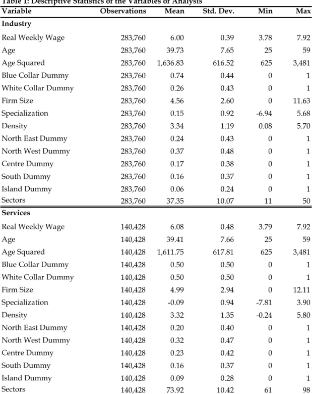
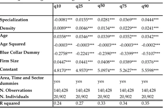
Table 1 sets out the descriptive statistics of the analysis variables, while Tables 2 and 3 show the quantile estimates for the industry and service sectors respectively. The findings reveal that the impact of both density and specialization increases along the wage distribution of Italian workers.15 _{Moreover, these impacts are higher for the service} sector. In particular, the local specialization coefficients range from an elasticity of 0.1% at

13 _{Note that we keep in the estimation the penalty term as introduced in Koenker (2004), in order to be}

as close as possible to previous quantile fixed effects estimates. We also performed the estimates without penalty term, and results remain pretty the same. Further, standard errors are derived from the estimation of a heteroskedasticity consistent variance-covariance matrix. See Galvao and Monte-Rojas (2009), Galvao (2008), Chernozhukov and Hansen (2008), for further details on the estimation technique and its properties.

14 _{Wages have been deflated using the Consumer Price Index specific for blue collars and white collars}

(FOI index, Indice dei Prezzi al Consumo per le Famiglie di Operai e Impiegati, ISTAT). The base year is 2001.

15 _{The control variables in the regressions have the expected signs: wages shows a concave shape in age;}

the blue collar dummies are negative. θ θ θ θ θ θ θ θ θ

ε

δ

λ

ϕ

γ

γ

β

α

i B I Char Firmsize Spec Dens

w + + + + + + + + + =

the 10th _{percentile to 1.3% at the 90}th _{percentile for industry, and from -0.8% at the 10}th percentile to 4.4% at the 90th _{percentile for the service sector, with the differences between} the two percentiles being statistically different from zero. As for density, the elasticity estimates range from 1.3% at the 10th _{percentile to 2.1% at the 90}th _{for industry and from} 0.9% at the 10th _{percentile to 2.4% at the 90}th _{for the service sector. These findings suggest} that the impact of spatial externalities is not uniform along the wage distribution, the impact at the 90th _{percentile being greater than the impact at the 10}th _{percentile. This} finding is at odds with Wheeler (2007), who points out a reduction of wage inequality related to spatial externalities, while it falls in line with Moller and Haas (2003), who find an increasing impact of spatial externalities along the wage distribution.

As far as the impact of firm heterogeneity is concerned, the firm size elasticities are positive, as expected, and decrease slightly along the wage distribution, standing in the industry (service) sector at 4.3% (4.5%) at the 10th _{percentile and at 3.4% (3.8%) at the 90}th percentile. This evidence suggests that in cross-sectional quantile estimates the size of the firm favors the workers located at the bottom more than those at the top of the wage distribution.

[Table 1 around here] [Table 2 and 3 around here]

5.1.2 Unobserved Heterogeneity: the Quantile Fixed Effects Estimates

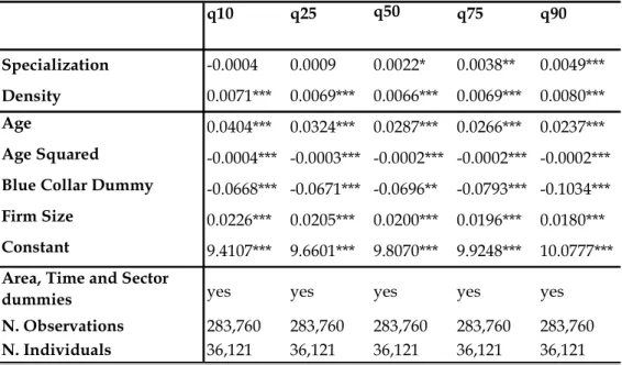
We then perform quantile fixed effect estimates to control also for the unobserved worker heterogeneity (Koenker, 2004). Table 4 and 5 show that previous results change when taking into account the relevance of worker sorting, proxied by the individual fixed effects. The coefficients of the spatial variables are considerably reduced compared to the previous quantile estimates and, in some cases, they are even no longer statistically different from zero.

As far as density is concerned, in the industry sector coefficients are reduced and become basically stable along the wage distribution. This evidence suggests that the impact of sorting is stronger at the highest quantiles since, in the cross-sectional analysis, the impact was increasing along the wage distribution.16 _{In the service sector coefficients} remain positive only in the right tail of the wage distribution, while they are no different from zero up to the median. Also in this case sorting matters, and again it mostly affects the highest percentiles of the wage distribution. It is worth noting how striking the

16 _{The differences among coefficients at different percentiles are not statistically different from zero}

coefficient reduction proves: the elasticity for the employment density is reduced by more than 60% in the industry sector at the 90th _{percentile (from 2.1% to 0.8%) and by} around 75% in the service sector (from 2.4% to 0.6%). According to these findings, density entails only a slight positive impact on wage inequality in the service sector, while it no longer affects wage inequality in the industry sector.

As for specialization, it still has an increasing impact (even if much reduced) along the wage distribution of Italian workers, since the coefficients are either not statistically different from zero or negative from the 10th _{percentile to the median and positive in the} 75th _{and 90}th _{percentiles. In particular, in the industry sector the coefficient estimates are} reduced by more than 50% in the right tail of the wage distribution, falling from 0.9% (1.3%) to 0.4% (0.5%) at the 75th ₍₉₀th_{) percentile. In the service sector the coefficient} reduction is even more striking. The coefficient estimates in the right tail of the wage distribution decrease by around 90%, from 3.7% (4.4%) to 0.3% (0.4%) at the 75th ₍₉₀th₎ percentile, while coefficients are still negative in the lower part of the distribution. This means that specialization favours skilled workers and penalizes unskilled ones.

The results of the quantile fixed effects estimates indicate that sorting matters and captures most of the impact of spatial externalities. Nonetheless, even after controlling for sorting there is still evidence of a increasing impact of spatial externalities along the wage distribution. These latter findings are consistent with the idea in Glaeser and Maré (2001) and Glaeser and Resseger (2010) that skilled workers are attracted by cities and cities make skilled workers more productive, being more adept at gaining from face-to-face interactions and from faster human capital accumulation. Our findings are also in line with Glaeser et al. (2009), who focus on the causes of urban inequality in the US. Using aggregate measures of inequality, they underline that individual skills (in terms of education) account for one third of the variation in income inequality (proxied by the Gini index) across metropolitan areas.

As for the impact of firm heterogeneity, Tables 4 and 5 show that the firm size coefficients are still decreasing along the wage distribution, but much reduced -by around 50%- compared with those derived in cross sectional quantile estimates. This suggests that the individual fixed effects capture a relevant part of the premia related to firm size.

5.1.3. Endogeneity Issues: IV Quantile Fixed Effects Estimates

To take into account the endogeneity bias arising from the simultaneity in the individual choices concerning wages and locations, we make use of a very recent IV quantile fixed effects methodology (Galvao and Montes-Rojas, 2009, Galvao, 2008, Harding and Lamarche, 2009).

For the instruments, we resort to deeply lagged variables, as in Ciccone and Hall (1996), Combes et al. (2008), Combes et al. (2010a) and Mion and Naticchioni (2009). The intuition is that deeply lagged levels of specialization and density are correlated to the current levels of spatial variables, although they are supposed not to influence productivity and wages today. The efficacy of using deeply lagged variables as instruments is provided in Combes et al. (2010a), who show that, for both wages and firm TFP spatial regressions, deeply lagged variables perform at least as well as other instruments (like detailed soil and climate information) that are a priori more closely related to the local determinants of the old rural population.

As deeply lagged variables we use, for density, the value of density in 1861 and 1881 and, for specialization, the value of specialization in 1951. These instruments variables refer to time periods prior to the Golden Age of the Italian economy, started in the late fifties, and hence prior to the development of the current economic structure and to the start up of the Italian industrial districts system.More specifically, we use as instruments ĝ the least square projections of the endogenous variables d on the deeply lagged values of the spatial variables g.17

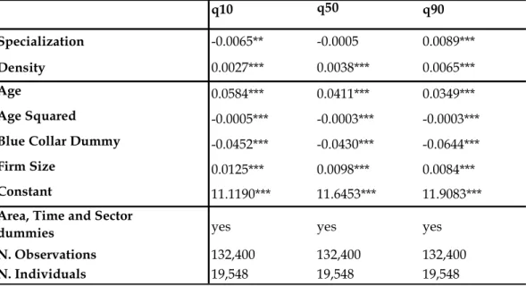
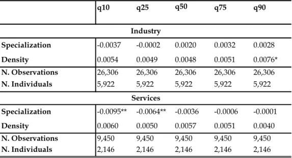
We perform the estimation simultaneously on three quantiles, the 10th, the 50th and the 90th_{. Results are shown in Tables 6 and 7 for the industry and service sectors,} respectively. As for industry, Table 6 shows that coefficients turn out to be slightly reduced in magnitude compared to previous quantile fixed effects estimates (Table 4). In particular, the impact of specialization is positive and significant again only at the 90th percentile, thus confirming previous findings. The impact of density is also very close to quantile fixed effects coefficients. However, unlike quantile fixed effects estimates, the coefficients at the 10th _{and 90}th _{percentiles are statistically different one another, and} therefore the impact of density now increases along the wage distribution.

17

By doing so, the equation is exactly identified, and it is possible to use as weight matrix in the minimization formula (6) the identity matrix (see Galvao and Montes-Rojas, 2009, Galvao, 2008, and Chernozhukov and Hansen, 2008). Moreover, since in this procedure it is not possible to test whether the instruments are weak, we perform a standard IV fixed effects regression and we look at the F-statistics of the first stage. Results highlight that, for both industry and service sectors, instruments have F-statistics values well above the standard threshold of 10, consistently with Mion and Naticchioni (2009).

Also for the service sector, the patterns of the spatial variables confirm those obtained using quantile fixed effects estimates (Table 7). In particular, for specialization the impacts is negative at the 10th _{percentile and positive at the 90}th _{percentile, with a larger} difference between the two coefficients with respect to Table 5, i.e. a more unequal impact of specialization along the wage distribution. The coefficients for density are now always positive and increase along the wage distribution.

As for firm size, coefficients are quite close to previous ones, i.e. firm sorting has a decreasing impact on the wage distribution.

To sum up, even after taking into account endogeneity issues, our findings suggest that the sorting of workers is the most important factor behind the relation between spatial variables and wage distribution, and that the impact of spatial variables is increasing along the wage distribution. Our findings extend to the whole wage distribution the results of Combes et al. (2010a): spatial variable impact on wages is only slightly affected by endogeneity bias (in their terminology, the ‘endogenous quantity of labour’ problem), while it is strongly affected by the sorting of workers (‘the endogenous quality of labour’ problem).

[Table 6 and 7 around here]

5.2 Robustness Checks

In this section we present a set of robustness checks.

First, it could be argued that the quantile fixed effects estimates might be biased since they are mainly identified by movers, i.e. workers who change location and/or industry. The empirical literature showed that movers are likely not to be a random sample of the workforce since their mobility choices can be due to different reasons, such as improving their occupations while employed or looking for a new job either because they have been fired or because their firms have closed down. This heterogeneity in mobility choices might entail selection problems, and hence a bias in the estimates. Therefore, we carry out the quantile fixed effects estimates on the sample of the displaced workers (as in Dustmann and Meghir, 2005, and Mion and Naticchioni, 2009) since, by assuming that firm closure is exogenous conditional on observables, it represents a random sample of the workforce. This strategy has to be considered as another attempt to deal with endogeneity issues and sample selection. Table 8 shows even more striking results, since the reductions in coefficients are greater (in magnitude) than in previous quantile fixed effects estimates, and the coefficients are in general not statistically significant. These findings suggest that sorting captures all the effects related to spatial externalities.

However, it is worth noting that the sample of displaced workers over-represents some worker characteristics of the original sample. In particular, the percentage of blue-collar workers is higher in the sample of displaced workers, and this is likely to explain, at least partially, the difference between the results of these estimates and the previous ones. For this reason, even if the estimates on the sample of displaced workers amply confirm the importance of the sorting of workers, we consider the quantile fixed effects estimates on the whole sample, set out in Tables 4 and 5 (and the related IV estimates set out in Tables 6 and 7), as the estimates to be preferred.

The second robustness check concerns the choice of the quantile fixed effects methodology. Instead of using the procedure of Koenker (2004) we implement another technique proposed by Arulampalam et al. (2008) and also implemented by Bache et al. (2008). It is a two-stage procedure where, in the first stage, a standard within-panel regression is performed to produce an estimate of the fixed effects. In the second stage, a simultaneous quantile estimation is carried out, adding as explanatory variables the fixed effects estimated in the first stage. Though the asymptotic properties of this estimator are still unknown, it performs well and is simple to implement (Bache et al., 2008). We rely on bootstrap for the coefficients and standard errors estimates, as in Bache et al. (2008). The results of this two-stage procedure largely confirm the findings of the Koenker’s one (Table 9).

The third robustness check focuses on firm heterogeneity, proxied in our analysis by firm size. We carry out two different checks. First, we perform the fixed effects quantile estimates (Koenker, 2004) adopting a finer specification for the firm size. In particular, we run the estimates with an interaction effect between (20) regional dummies and the firm size. This allows us to capture better the heterogeneity in the firm size returns – a heterogeneity that might depend on the considerable regional differences that characterize the Italian labour market. Second, we perform the quantile fixed effects estimates excluding firm size in order to verify whether the possible collinearity between firm size and density (which is very low indeed in our sample, around 0.13) affects the impact of density on wages. The results of both these robustness checks are much the same as those in Tables 4 and 5, confirming previous findings. We do not provide these estimates here for the sake of synthesis; they are available upon request.18

18 _{We also perform a two-stage estimation technique in order to look at the impact of the spatial}

variables on an aggregate measure of inequality, the Gini index. We first run a fixed effects estimate of wages on the worker observable characteristics (age, age squared, blue collar dummy) and on the firm size. Then, we compute the Gini index at provincial-sectoral level by using the residuals (εi,t) of this first

stage regression. We then regress the Gini index on the spatial variables controlling for provincial-sectoral dummies. We also run the same procedure using the joint residuals (the residuals plus the fixed effects estimates, εi,t+ui). The results largely confirm the findings derived using individual data. As

[Table 8 and 9 around here]

6. The Characteristics of Sorting

6.1 Sorting and its Distributional Patterns

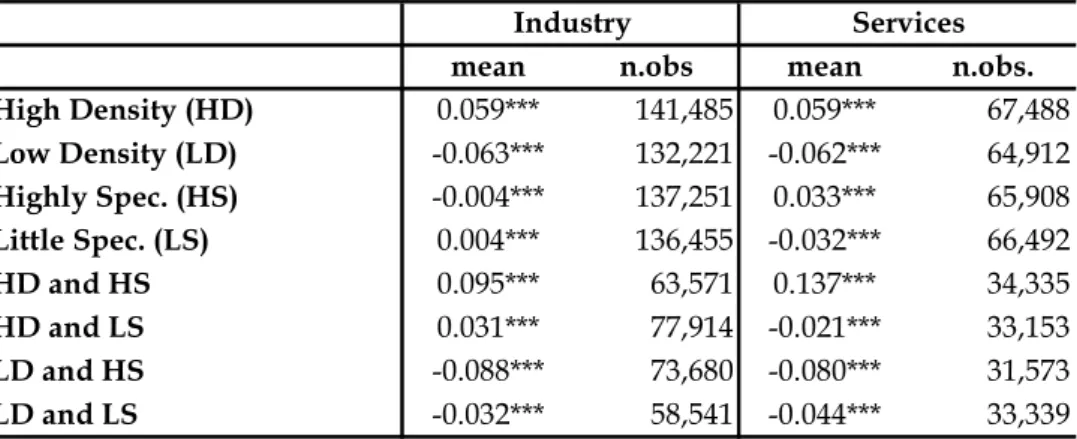
The aim of this section is to investigate the characteristics of the sorting of workers, looking into the distribution of the individual fixed effects – our measure for time-invariant individual skills – among high and low density provinces, as well as among highly and little specialized provinces. We first split provinces into low density (LD) and high density (HD), and little specialized (LS) and highly specialized (HS), on the basis of the median of the (time average of) density and specialization in our database. We then use the individual fixed effects obtained from our preferred specification, the quantile IV fixed effect estimates of Table 6 (for industry) and 7 (for services), to derive summary statistics of the distribution of skills in HD, LD, HS and LS provinces (Table 10). As for density, workers in HD provinces display higher average skills than those in LD provinces, in both the industry (0.059 vs -0.063) and service sector (0.059 vs -0.062).19 Moreover, the difference in skill averages between HD and LD provinces is even greater when these provinces are also HS (0.095 vs -0.088 for the industry and 0.137 vs -0.080 for the service sector), suggesting that, as expected, there is an interrelation between the effects of the two spatial variables. It is also possible to compute a rough measure of the extent to which the difference in the average (log) wages between HD and LD provinces (at the denominator) can be explained by the difference in the average fixed effects (at the numerator). We find that differences in fixed effects account for 77% of row spatial wage variation between HD and LD provinces in the industry sector and for 79% in the service sectors – measures similar to those described in Mion and Naticchioni (2009) (nearly 75% for all the economy).

For specialization, Table 10 shows that workers in HS provinces are more skilled than those in LS provinces only in the service sector (0.033 in HS vs -0.032 in LS). In the industry sector, the difference in skills between HS and LS provinces is negligible (it becomes more relevant when this difference is considered in HD provinces: 0.095 vs dependent variable εi,t+ui), spatial variables entail a strong, positive and significant impact on wage

inequality, while when taking into account the role of sorting (using only the εi,t residuals), density no

longer entails any significant impact on wage inequality, while specialization still does so. As for the service sector, spatial variables have positive and significant impacts on the Gini index – impacts that are generally reduced when taking into account the unobserved individual heterogeneity. Moreover, when we run the same procedure using the IV estimates, we find out that both in the industry and service sectors, spatial variables entail a positive impact on wage inequality. We do not show these estimates for sake of synthesis. They are available upon request.

19 _{These findings are in line with Mion and Naticchioni (2009) who derive similar results for the two}

0.031). Further, in the case of specialization individual fixed effects account for 62% (88%) of the differences in row wage variation between HS and LS provinces in the industry (service) sector.

Taking into consideration the sorting of firm, we point out that it accounts for a much smaller fraction of wage differentials with respect to the sorting of workers. In fact, the differences in (log) wages between HD and LD provinces explained by firm sorting is 7.4% (5.4%) for the industry (service) sector, while between HS and LS provinces it is 1.1% (0.4%) for the industry (service) sector. These findings are also in line with those in Mion and Naticchioni (2009), who show that firm sorting accounts for only 5.6% of row spatial wage variation along the density dimension. For this reason, we will investigate the relevance of firm sorting no further in this paper.

[Table 10 around here]

Let us now return to the main focus of the paper, the distributional consequences of the agglomeration externalities and the role of sorting. In order to characterize further the stronger impact of sorting in the upper tail of the wage distribution, we compute summary statistics on the distribution of the individual fixed effects between HD and LD, and between HS and LS, provinces, by terciles of the wage distribution (0-33, 33-66, 66-100, Table 11). First of all, it is worth noting that, as expected, the individual fixed effects are on average negative for workers belonging to the lowest wage tercile, close to zero for those in the central tercile, and positive for workers belonging to the highest tercile. Second, in the top tercile of the wage distribution (Panel C) the number of observations is much higher in the HD provinces than in the LD provinces. Conversely, in the bottom tercile (Panel A) the number of observations in the LD provinces is higher than in the HD provinces. This confirms the presence of a composition effect, i.e. high paid (low paid) workers are concentrated in HD (LD) provinces. Third, the difference in the average skill levels of workers located in HD (HS) and LD (LS) provinces is noteworthy only when taking into account the highest tercile. In fact, while in the bottom and medium terciles the differences of the averages fixed effects between high and low density (specialized) provinces are close to zero (Panel A and B of Table 11), in the top tercile (Panel C) the average skills are greater in HD (HS) provinces.20 _{This finding confirms that sorting is at} work and explains the coefficient drop detected in quantile fixed effects estimates for the right tail of the wage distribution. Fourth, the averages of the fixed effects are higher in the service sector, confirming that this sector attracts a greater number of skilled workers. This explains why in the cross-sectional quantile estimates the impact of spatial

20

In particular, as for density in the industry sector, the difference in skills levels between workers in HD and LD provinces is 0.05, while it comes to 0.02 in the service sector. For specialization, the difference in the highest tercile in skill averages between workers employed in HS and LS provinces is 0.02 in the industry sector and 0.06 in the service sector.

externalities was stronger in the service sector, and why the service sector saw the greater coefficient drop in the quantile fixed effects estimates.

[Table 11 around here]

6.2 Sectoral Breakdown of Sorting

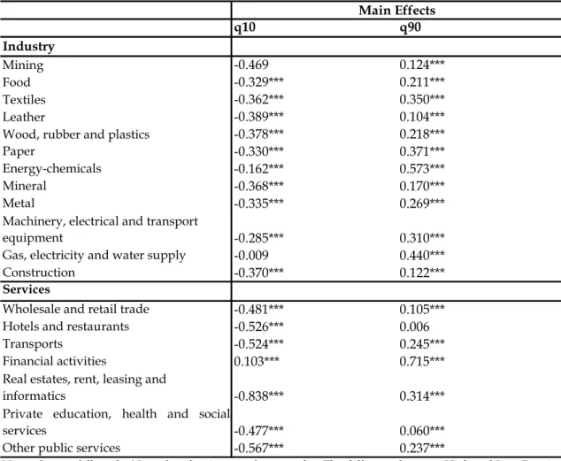
In this section we set out to characterize the sorting of workers among the different sectors of the economy in order to address two main issues.21 _{First, we wish to investigate} whether the distributional patterns of the sorting of workers is homogeneous across sectors. Second, we aim at a better understanding of the impact of spatial externalities in the service sector, which represents a relatively unexplored research field within the spatial economic literature. To the best of our knowledge, no papers have focused on the sectoral breakdown of the sorting of workers. Our variable of interest is the individual skill, proxied by the individual fixed effects computed in our preferred specification (IV quantile fixed effects, Table 6 and 7 for industry and services, respectively). Instead of carrying out a set of cumbersome descriptive statistics across provinces and sectors, we regress the individual fixed effects on sectors dummies, dummies for both high density and highly specialized provinces (HD and HS), and interaction terms between sectors and spatial (both HD and HS) variables.

Since our main concern is on distributional issues, we run quantile regressions on the 10th _{and the 90}th _{percentiles. By doing so, we can identify the skill intensity by sector,} provided by the coefficient of each sector dummy (when both HD and HS are equal to zero). Table 12 shows that at the 90th _{percentile the skill levels are generally higher in the} skill-intensive sectors such as ‘energy-chemicals’, ‘paper’, ‘machinery, electrical and transport equipment’, ‘gas, electricity and water supply’ for industry, and ‘financial activities’, ‘real estates, rent, leasing and informatics’ for the service sector.

[Table 12 around here]

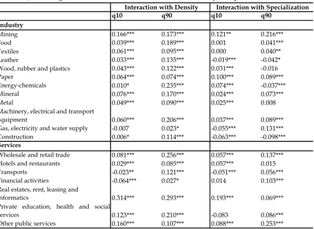
Table 13 shows for each quantile and each sector the difference in skill levels between being in an HD (HS) province rather than an LD (LS) province, i.e. the coefficients of the interaction terms.22 _{By doing so we can identify which are the sectors characterized by the}

21 _{For this analysis we follow the NACE rev. 1.1 classification, two letters codes, which identifies 19}

sectors derived aggregating the 51 sectors used so far with the Ateco81 classification.

22 _{More specifically, the coefficients of the interaction terms between sectors and HD (HS) dummies}

refer, for each sector, to the difference in skill levels when passing from the omitted category (both HD and HS dummies equal to zero) to an HD (HS) province.

highest incidence of worker sorting – sectors that represent the driving force behind the impact of sorting detected in the previous sections.

As for density, two main findings emerge from Table 13, for both industry and services. First, regardless of the quantile considered there is evidence of sorting in almost all sectors since the coefficients are mainly positive. Second, the sorting of workers increases along the wage distribution, i.e. the coefficients at the 90th _{percentile are greater} than those at the 10th _{percentile, in all sectors apart from ‘other public services’. These} findings suggest that in dense provinces skilled workers benefit the most from the advantages related to urban agglomeration externalities (Glaeser and Maré, 2001, Glaeser and Resseger, 2010, Baum-Snow and Pavan, 2010).

Also for specialization Table 13 shows that there is strong evidence of sorting, most of the coefficients being positive. However, the patterns of sorting of workers when moving from the 10th _{to the 90}th _{percentile are heterogeneous among the different sectors.} Actually, some sectors show increasing sorting of workers (an increase in the coefficients from the 10th _{to the 90}th _{percentile), while others show negligible, or even decreasing,} patterns. As for industry, most of the sectors showing an increasing sorting of workers from the 10th _{to the 90}th _{percentile are characterized by low- and medium-skill intensity:} ‘mining’, ‘food’, ‘textiles’ and ‘mineral’.23 _{To arrive at an explanation for these findings it} is necessary to stress that in Italy unskill-intensive sectors are mostly located in highly specialized (and generally low density) provinces and are greatly involved in international trade, as also pointed out in Matano e Naticchioni (2008). Therefore, workers employed in these sectors in HS provinces are much exposed to international competition. According to Feenstra and Hanson (2003), international competition, i.e. trade in intermediate inputs and outsourcing activities, may generate the same impact on labour demand as skill-biased technical change, shifting away the demand for unskilled workers and raising the demand for the skilled. This theoretical framework is to some extent consistent with our findings: on the one hand, skilled workers benefit from international competition, since they receive a premium when moving from an LS to an HS province in these sectors, i.e. the coefficients at the 90th _{percentile are positive (Table} 13). On the other hand, coefficients for unskilled workers (at the 10th _{percentile) are either} zero or slightly positive, and lower than coefficients for other sectors less exposed to international competition. In the service sector, the difference in the average fixed effects in HS provinces with respect to LS ones is positive and increasing along the wage distribution for most of the sectors. It is also worth noting that the ‘wholesale and retail trade’ sector is characterized by the highest number of observations within services

23 _{The only exception in this framework is the ‘leather’ sector that, however, constitutes only the 2.24%}

(50,131 out of 132,400 for all services). For this reason we claim that this sector represents the driving force behind the coefficient drop at the 90th _{percentile when passing from the} cross sectional quantile regressions to the quantile fixed effects regressions in the service sector observed in Table 5 (and confirmed in Table 7). It is also interesting to underline that the skilled service sector ‘real estate, rent, leasing and informatics’, though displaying sorting at all percentiles, is characterized by smaller coefficients at the 90th percentile than those at the 10th _{percentile, i.e. in this sector sorting is more relevant for} the unskilled workers. This can be due to the fact that unskilled workers in this sector are able to capture higher advantages from agglomeration externalities due to learning mechanisms arising from the interactions with skilled workers, in line with Glaeser and Maré (2001) and Wheeler (2007).

[Table 13 around here]

7. Conclusions

In this paper we investigate the role that sorting plays in the relation between spatial externalities (in terms of industrial specialization and density) and wage distribution. Using Italian individual panel data and quantile fixed effects estimates (both standard and IV), we can derive estimates of the impact of spatial variables not affected by individual and firm heterogeneity, nor indeed by endogeneity arising from simultaneous individual choices concerning wage and locations. Our results show that the sorting of workers captures most of the impact of spatial externalities derived in standard quantile estimates and that its impact increases along the wage distribution. Nonetheless, even after controlling for worker sorting, there is evidence of a positive impact of spatial externalities on the wage distribution. As for firm sorting, it proves far less relevant than the sorting of workers. Finally, analyzing the sectoral breakdown of sorting, we demonstrate that it is not always homogeneous across sectors. More specifically, along the density dimension worker sorting is pervasive in all sectors, while along the specialization dimension it occurs mainly in low- and medium-skilled sectors, consistently with the international competition exposure explanation.

References

1. Abdel Rahman, H.M., Fujita, M. (1990), Product Variety, Marshallian Externalities and City Size, Journal of Regional Science, 30(2):165-183.

2. Abrevaya, J., Dahl, C. (2008), The effects of Birth Inputs on Birth-weight: Evidence from Quantile Estimation on Panel Data, Journal of Business and Economic Statistic, 26(4): 379-97.

3. Arulampalam, W., Naylor, R.A., Smith, J. (2008), Am I Missing Something? The Effects of Absence from Class on Student Performance, IZA Discussion Paper 3749. 4. Bacolod, M., Blum, B.S., Strange W.C. (2009), Skills in the City, Journal of Urban

Economics, vol. 65(2), pp. 136-153,

5. Bache, S.H., Dahl C. and Tang Kristensen J., (2008), Determinants of Birthweight Outcomes: Quantile Regression Based on Panel Data, CREATES Research Paper 2008-20, School of Economics and Management, University of Aahrus.

6. Bargain, O., Melly, B. (2008), Public Sector Pay Gap in France: New Evidence Using Panel Data, IZA Working Paper 3427.

7. Baum-Snow, N., Pavan, R. (2010), Understanding the City Size Wage Gap, processed, Brown University.

8. Brown, G., Medoff, J. (1989), The Employer Size Wage Effect, Journal of Political Economy, 97: 1027-1057.

9. Chamberlain, G. (1994), Quantile Regression, Censoring, and the Structure of Wages, in: Sims, C. (eds.): Advances in Econometrics: Sixth World Congress. 6, 1. Cambridge University Press: 405–437.

10. Chernozhukov, V., Hansen, C. (2008), Instrumental Variable Quantile Regression: A Robust Inference Approach, Journal of Econometrics, 142: 379–398.

11. Ciccone, A., Hall, R. (1996), Productivity and the Density of Economic Activity, American Economic Review, 86: 54-70.

12. Ciccone, A. (2002), Agglomeration Effect in Europe, European Economic Review, 46: 213-227.

13. Cingano, F. (2003), Returns to Specific Skills in Industrial Districts, Labour Economics, 10(2): 149-163.

14. Combes, P. (2000), Economic structure and local growth: France, 1984-1993, Journal of Urban Economics, 47: 329-355.

15. Combes, P., Duranton, G., Gobillon, L. (2008), Spatial Wage Disparities: Sorting Matters!, Journal of Urban Economics, 63: 723-742.

16. Combes, P., Duranton, G., Gobillon, L., Roux, S. (2010a), Estimating Agglomeration Economies with History, Geology, and Worker Effects, in Glaeser E.L. (ed.), Agglomeration Economics, NBER, Cambridge, MA.

17. Combes, P., Duranton, G., Gobillon, L. (2010b), The Identification of Agglomeration Economies, mimeo available at http://individual.utoronto.ca/gilles/research.html.

18. Di Addario, S., Patacchini, E. (2008), Wages and the Cities: Evidence from Italy, Labour Economics, 15(5): 1040-1061 .

19. Duranton, G., Puga, D. (2003), Microfoundations of urban agglomeration economies, in Henderson J.V. and Thisse J.-F. (eds.), Handbook of Regional and Urban Economics, 4, Elsevier North Holland, Amsterdam.

20. Dustmann, C., Meghir, C. (2005), Wages, Experience and Seniority, Review of Economic Studies, 72: 77-108.

21. Feenstra, C., Hanson, G. (2003), Global production sharing and rising wage inequality: a survey of trade and wages, in K. Choi and J. Harrigan (eds.), Handbook of International Trade, Basil Blackwell, 146-185.

22. Galvao, A., Montes-Rojas, G. (2009), Instrumental Variables Quantile Regression for Panel Data with Measurement Errors, Department of Economics Discussion Paper Series 09/06, City University London.

23. Galvao, A. (2008), Quantile Regression for Dynamic Panel Data, revised and resubmit for Journal of Econometrics, University of Illinois, Urbana-Champaign.

24. Glaeser, E.L., Kallal, H.D., Scheinkman, J.A., Shleifer, A. (1992), Growth in Cities, The Journal of Political Economy, 100(6): 1126-1152.

25. Glaeser, E.L., Maré, D.C. (2001), Cities and Skills, Journal of Labor Economics, 19(2): 316-342.

26. Glaeser, E.L., Resseger, M.G., Tobio, C. (2009), Inequality in Cities, Journal of Regional Science, vol 49(4), pp. 617-646.

27. Glaeser, E.L., Resseger, M.G. (2010), The Complementarity Between Cities and Skills, Journal of Regional Science, vol. 50(1), pp. 221-244.

28. Gould, E. (2007), Cities, Workers, and Wages: A Structural Analysis of the Urban Wage Premium, Review of Economic Studies, 74, 477-506.

29. Harding, M., Lamarche, C. (2009), A Quantile Regression Approach for Estimating Panel Data Models Using Instrumental Variables, Economic Letters, 104: 133-135. 30. Helsley, R., Strange, W. (1990), Matching and Agglomeration Economies in a System

of Cities, Regional Science and Urban Economics, 20(2): 189-212.

31. Kim, S. (1989), Labor Specialization and the Extent of the Market, Journal of Political Economy, 97(3): 692-705.

32. Koenker, R. (2004), Quantile Regression for Longitudinal Data, Journal of Multivariate Analysis, 91(1): 74-89.

33. Koenker, R., Bassett, G. (1978), Regression Quantiles, Econometrica, 46: 33-50.

34. Krueger, A.B., Summers, L.H. (1988), Efficiency Wages and the Inter-Industry Wage Structure, Econometrica, 56(2): 259-293.

36. Matano, A., Naticchioni, P. (2008), Trade and Wage Inequality: Local vs Global Comparative Advantages, Working Paper DE-ISFOL 6, Sapienza Università di Roma, forthcoming in World Economy.

37. Melitz, M. (2003), The Impact of Trade on Intra-Industry Reallocations and Aggregate Industry Productivity, Econometrica, 71(6): 1695-1725.

38. Mion, G., Naticchioni, P. (2009), The Spatial Sorting and Matching of Skills and Firms, Canadian Journal of Economics, Canadian Economics Association, 42(1): 28-55.

39. Moller, J., Haas, A. (2003), The Agglomeration Differential Reconsidered: an Investigation with German Micro Data 1984-1997, in Broecker, J., D. Dohse, R. Soltwedel (eds.), Innovation Clusters and Interregional Competition. Berlin: Springer. 40. Moretti, E. (2004), Human Capital Externalities in Cities, in Henderson J.V. and Thisse

J.F. (eds.), Handbook of Regional and Urban Economics, Elsevier-North Holland, Amsterdam, 4.

41. Postel-Vinay, F., Robin, J.M. (2006), Microeconometric Search-Matching Models and Matched Employer-Employee Data, in R. Blundell, W. Newey and T. Persson (eds.), Advances in Economics and Econometrics: Theory and Applications, Ninth World Congress, 2, Cambridge: Cambridge University Press.

42. Rosenthal, S.S., Strange, W.C. (2004), Evidence on the Nature and Sources of Agglomeration Economies, in J.V. Henderson and F.Thisse (eds.), Handbook of Regional and Urban Economics, 4, Elsevier-North Holland, Amsterdam.

43. Topel, R. (1991), Specific capital, mobility, and wages: Wages rise with job seniority, Journal of Political Economy, 99: 145-176.

44. Wheeler, C.H. (2004), Wage Inequality and Urban Density, Journal of Economic Geography, 4: 421-437.

45. Wheeler, C.H. (2007), Industry Localization and Earnings Inequality: Evidence from US Manufacturing, Papers in Regional Science, 86(1): 77-100.